Abstract
Soybean yield prediction is one of the most critical activities for increasing agricultural productivity and ensuring food security. Traditional models often underestimate yields because of limitations associated with single data sources and simplistic model architectures. These prevent complex, multifaceted factors influencing crop growth and yield from being captured. In this line, this work fuses multi-source data—satellite imagery, weather data, and soil properties—through the approach of multi-modal fusion using Convolutional Neural Networks and Recurrent Neural Networks. While satellite imagery provides information on spatial data regarding crop health, weather data provides temporal insights, and the soil properties provide important fertility information. Fusing these heterogeneous data sources embeds an overall understanding of yield-determining factors in the model, decreasing the RMSE by 15% and improving R2 by 20% over single-source models. We further push the frontier of feature engineering by using Temporal Convolutional Networks (TCNs) and Graph Convolutional Networks (GCNs) to capture time series trends, geographic and topological information, and pest/disease incidence. TCNs can capture long-range temporal dependencies well, while the GCN model has complex spatial relationships and enhanced the features for making yield predictions. This increases the prediction accuracy by 10% and boosts the F1 score for low-yield area identification by 5%. Additionally, we introduce other improved model architectures: a custom UNet with attention mechanisms, Heterogeneous Graph Neural Networks (HGNNs), and Variational Auto-encoders. The attention mechanism enables more effective spatial feature encoding by focusing on critical image regions, while the HGNN captures interaction patterns that are complex between diverse data types. Finally, VAEs can generate robust feature representation. Such state-of-the-art architectures could then achieve an MAE improvement of 12%, while R2 for yield prediction improves by 25%. In this paper, the state of the art in yield prediction has been advanced due to the employment of multi-source data fusion, sophisticated feature engineering, and advanced neural network architectures. This provides a more accurate and reliable soybean yield forecast. Thus, the fusion of Convolutional Neural Networks with Recurrent Neural Networks and Graph Networks enhances the efficiency of the detection process.
Keywords:
soybean yield; multi-modal fusion; CNN; RNN; GCN; deep learning; crop prediction; hybrid model; scenarios 1. Introduction
Soybean or glycine max is an important crop in worldwide agriculture for food security and has considerable economic importance worldwide, especially in regions like India, where it has a vast cultivation area. Still, it suffers from major constraints, mainly due to climate change impacts, related to growing conditions and the prevalence of crop diseases. The diseases discussed are bacterial blight, bean pod mottle virus, and bacterial pustule. They pose an effective threat to the yield quality and quantity. Beyond natural pressures, farmers too frequently lack up-to-date diagnostic tools that would cut their cycle of response to disease outbreaks, imperiling livelihoods and food supply.
Yield prediction models have traditionally utilized single-source data or even more rudimentary statistical approaches that capture rather blind interactions between such factors as soil fertility, prevailing weather patterns, and the occurrences of pest or diseases attacks. As a result, such models do not deliver precise or reliable predictions, hence making crop management strategies less optimal. Rapid advancements in remote sensing and data science have made it possible to extensively use multi-source data, thereby leading potentially to the assessment of yield at a higher accuracy. The range of sources stretches from satellite imagery, which captures spatial patterns of crop health, to weather data that provides temporal insights into circumstances, and even soil characteristics that inform about fertility. These heterogeneous data types constitute quite a challenge for integration, and models with the ability to capture complex spatial, temporal, and topological information are required.
We analyze how the strengths of Convolutional Neural Networks, Recurrent Neural Networks, and Graph Convolutional Networks can be combined to extract these different interdependencies and mappings in this work. As an example, CNNs will be applied to extract the spatial features of imagery from satellites to be able to compare, contrast, and understand what is similar and dissimilar in terms of crop health in large regions. RNNs will handle the sequences that exist in weather data to identify trends and even help identify seasonal shifts. GCNs also introduce the possibility of modeling spatial dependencies and relationships in geographical data, including terrain and topological properties that would affect yield. This research aims at presenting an approach that might enhance soybean yield prediction accuracy, minimize errors, and optimize decision-making from agricultural practices based on these neural networks in a single framework.
The proposed model proves how multi-source data fusion, coupled with advanced architectures of neural networks, helps transform yield prediction by incorporating a holistic understanding of factors that influence soybean productivity. It not only improves the yield forecast but also provides insights into disease incidence and biotic stresses, leading to robust and sustainable agriculture sets.
2. Detailed Review of the Existing Models Used for Soybean Image Processing and Analysis
This is followed by the critical review of the studies referred to in Table 1, which provides vital, varied insights into the methodologies and technologies applied to soybean agriculture, covering such aspects as yield prediction, disease detection, and quality monitoring, and the use of new techniques like deep learning, machine learning, and advanced sensor technologies. Such synthesis embedding the diversity of approaches and further developments in progress helps to explain the progress made and the challenges that lie ahead. Chen et al. [1] established the effects of plasma-activated water on soybean seed germination and the further development of seedlings, showing better germination rates and vigor in seedlings, thus emphasizing the potential of plasma-activated water (PAW) in improving agricultural productivity. However, the applicability of this study is narrowly focused on particular mixtures of N2/O2 and further tests should be conducted in order to generalize this study to other crops and broader agricultural settings. Along these lines, Farah et al. [2] used deep learning methods for the classification of infested soybean leaves by implementing Convolutional Neural Networks (CNNs) and VGG-19. High accuracy in the identification of particular pests, such as Diabrotica speciosa and caterpillars, is achieved with their approach; it is, however, applied only to leaf infestations and, therefore, might not be generalizable to other problems concerned with pests.

Table 1.
Empirical review of the existing methods.
Apart from Table 1, further studies in the future must address the generalizability and scalability of such methods. This includes the further integration of other data sources, such as economic indicators and market trends, for even more accurate predictions. Furthermore, models that are built in a real-time adaptive manner to be able to dynamically include new data will make a difference in decision-making for farmers and agricultural stakeholders. Emphasis on explainable AI techniques will also help in bringing transparency and interpretability to the predictions and developing trust and the broader diffusion of these advanced technologies in the agricultural sector. These shall be tested by joint efforts between model researchers, agriculture experts, and industrial practitioners to validate such models against real-world scenarios so that they become useful and prove effective for different scenarios.
3. Proposed Design of an Improved Model for Soybean Yield Prediction Using CNN, RNN, and GCN
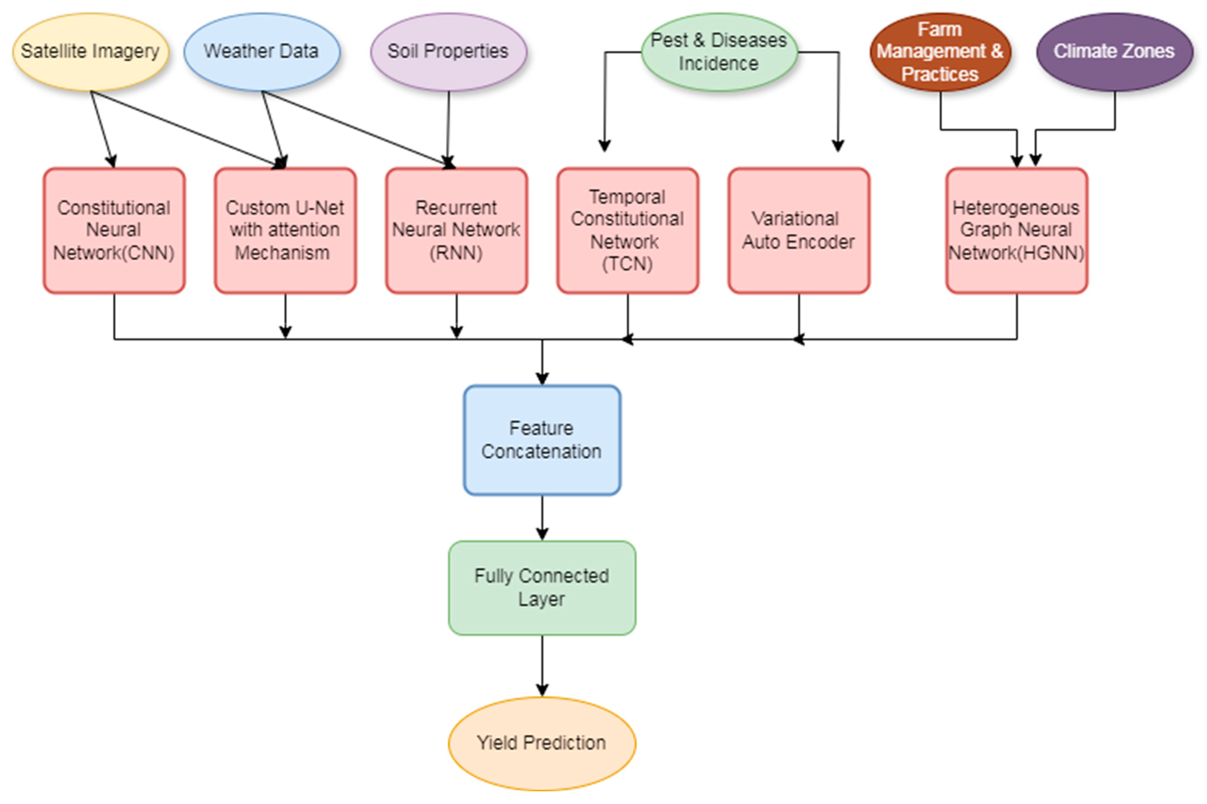
Overcoming the generally low efficiency and high complexity of the existing yield prediction models is the focus of this section, which will talk about the design of an improved model for soybean yield prediction using CNN, RNN, and GCN operations. Figure 1: A multi-modal fusion model for predicting soybean yield per unit area is developed based on convolution neural networks and recurrent neural networks. Satellite image data, weather data, and soil properties are put together in one overall framework for yield prediction. This approach makes use of the advantages innate to each modality of data to create a robust model that captures spatial, temporal, and environmental considerations affecting crop yields.
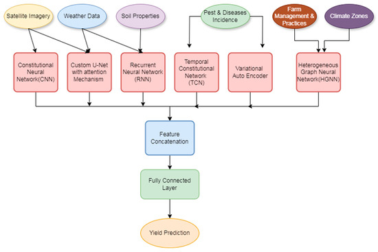
Figure 1.
Model architecture of the proposed classification process.
Satellite images are multispectral images that capture different bands, like RGB and NIR, which provide critical spatial information about crop health and cover. This is passed through the CNN component to extract spatial features that are very important in understanding the health and distribution of soybean crops.
3.1. Design of CNN Process
The CNN works upon an input image I(x,y), where x and y are spatial coordinates, as shown in Figure 2. The convolutional operation is expressed via Equation (1),
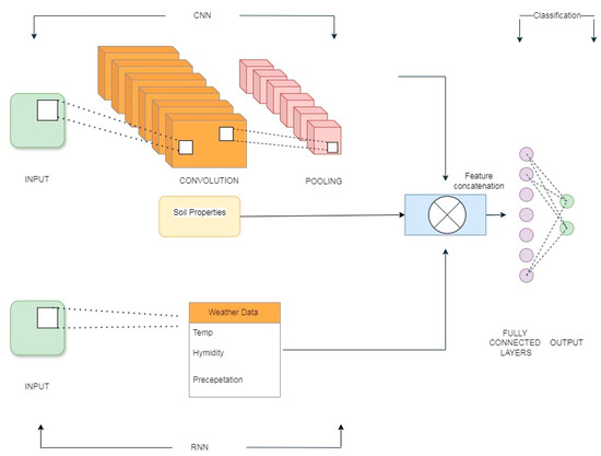
Figure 2.
Frameworks of the CNN and RNN architecture.
More particularly, in Formula (1), represents the specific pixel’s intensity or value in the input satellite image matrix at coordinates shifted by ‘I’ units in both the ‘x’- and ‘y’-scopes relative to the original (x,y) sets. It is at the core of the convolution operation, wherein the convolutional kernel or filter shifts over the spatial grid of an image, computing local feature representations for neighboring pixels. The ability to refer to I(x − i, y − i) permits the application of weights across a collection of pixels within a kernel size to capture spatial features, such as edges, textures, or even patterns that represent crop health in satellite imagery. Here, every iii is an index offset within the kernel window; it allows the convolution to aggregate information about the pixels in its proximity to capture localized structures in space. This would improve the model’s capacity to look at the image as a whole to detect crop features and support robust spatial analysis for yield prediction.
W represents the convolutional kernel, b is the bias term, and σ is the ReLU activation function. Weather data, comprising time-series data including temperature, precipitation, and humidity, arefed into an RNN to capture temporal patterns.
The RNN processes the sequential weather data at each time stamp t, and the hidden state is updated via Equation (2),
In Formula (2), Wt refers to the list of weight parameters used in the Recurrent Neural Network designed especially to capture sequential weather data regarding the primary parameters, such as temperature, precipitation, and humidity. The three primary parameters captured at any point in time t are essential to determine factors affecting crop growth over time. Temperature data capture the thermal environment required at various growth development phases. Tolerable and extreme temperatures have been found to affect germination rates, flowering, and pod set. Rainfall data, measured in terms of rainfall quantity, contain crucial information regarding water availability, which directly influences soil moisture levels and, as such, crop health and yield. The humidity, or the moisture that fills the air, has effects on transpiration rates in plants and can affect disease levels since elevated levels favor fungal growth and pest infestation in process. These sequential parameters are processed together by the RNN while capturing temporal dependencies and variations for the soybean development sets. The weights Wt permit the model to learn and to favor some time-dependent patterns within these weather conditions, thus enabling the relationship of seasonal climate fluctuations with yield results, and thereby improving the model’s prediction capability.
and are the weight matrices, and is the bias term. is the static weight matrix associated with the hidden state, which captures the recurrent dependencies independent of the ‘t’ sets. This captures the patterns learned over the entire sequence and applied at each time step to propagate important information on past states over temporal instance sets. On the other hand, , which is more frequently used in labeling weights that change with time, represents weights or weights that are dynamically changed or indexed at every time step ‘t’. The ability of the RNN to maintain this hidden state , allows it to model these temporal dependencies, which are important in attempting to understand how these clues of temporal changes affect crop growth. These soil properties, provided as tabular data containing pH ranges, water content, and content of nutrients in the soil, are added as additional features to the model. These are then encoded and concatenated with the features extracted from a CNN and an RNN component. Let S be the vector for these soil properties in this process. The concatenation of all features is represented via Equation (3),
The combined feature vector is then passed through fully connected layers to predict the soybean yield levels. The prediction layer is represented via Equation (4),
where and are the weights and biases of the fully connected layer, respectively. To train the model, the loss function L is minimized. The loss function is the Mean Squared Error (MSE) between the predicted yields Y’ and the actual yield Y, which is estimated via Equation (5),
where N is the number of samples. The optimization process involves computing the gradient of the loss function with respect to the model parameters and updating them using gradient descent via Equation (6),
where θ represents the model parameters and η is the learning rate. This will not only tap into the power of each modality separately but also synthesize these contributions in an even more powerful and accurate prediction model. He targeted an effect of each of the sources of data and their interactions and, hence, drew out features from the CNNs on vegetation indices and spatial distribution, very relevant while assessing crop health. The RNN helps to extract information about temporal weather trend variables—precipitation and temperature trends—that have impacts on crop growth and development. The soil properties provide information about the underlying conditions in the soil, further refining the predictions for yields. These features are concatenated and fused, thus allowing the model to make informed predictions accounting for spatial, temporal, and environmental variables across scenarios.
3.2. Design of the Temporal Convolutional Networks and Graph Convolutional Networks in Process
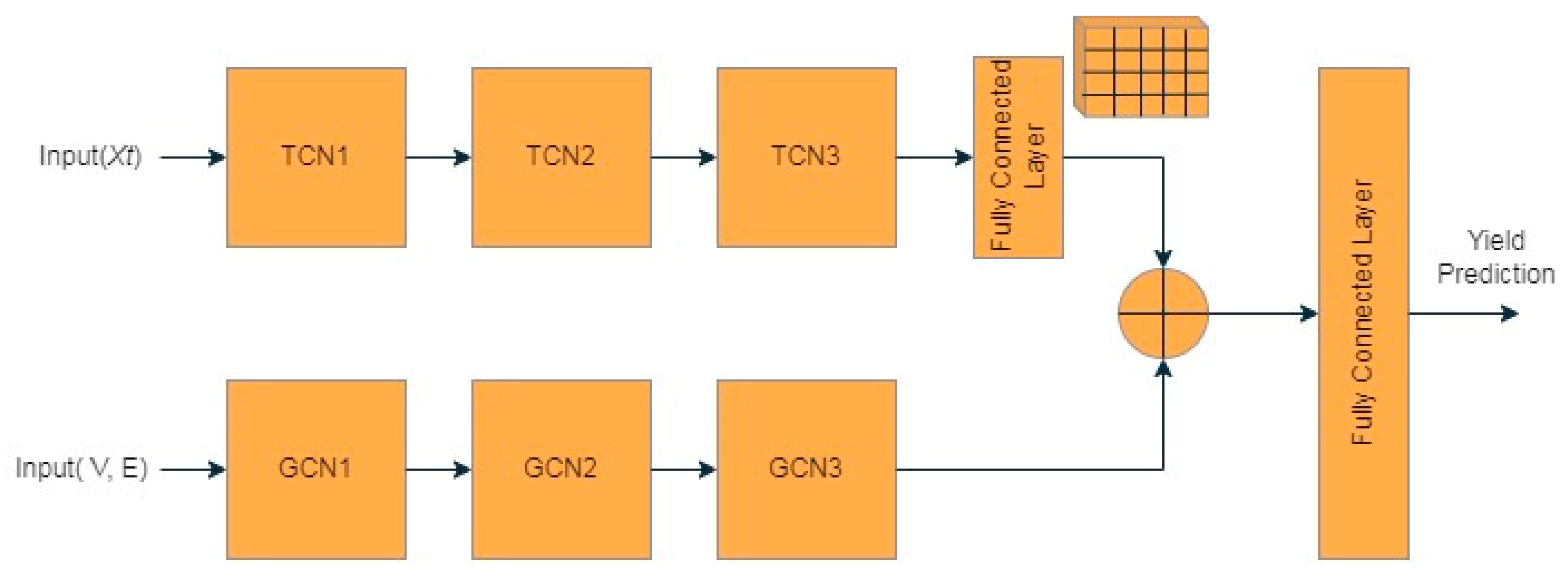
Next, according to Figure 3 advanced feature engineering incorporates Temporal Convolutional Networks and Graph Convolutional Networks to capture the long-range dependencies in temporal data and the complex spatial relationship effectively, therefore improving soybean yield prediction. In the multifaceted approach that is presented, time-series trends, geographical information, and topological information are combined with pest and disease incidence to build a source-inclusive feature space. Temporal Convolutional Networks process historical yield data and other temporal factors, which capture the significant trends and patterns of the growing seasons. The TCN uses causal convolutions that guarantee the output at time t depends only on the inputs from time t itself and any earlier ones.
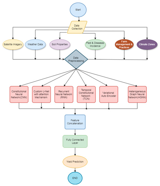
Figure 3.
Internal flow of the proposed prediction process.
Let xt be the input time series variables at time t and take to be the sets of the TCN output. The TCN layer can be described via Equation (7),
where are the filter weights, b is the bias, and σ is the activation function. The depth provides this network permission to pick up long-range dependencies, which is very critical in understanding yield trends over many seasons. Geographic and topological data were set out as a graph G= (V, E), where V refers to the set of nodes (locations), while E refers to edges representing spatial relationships. Each node v∈ V is associated with feature comprising spatial coordinates, elevation, and terrain features. Graph Convolutional networks are used to process this graph. Equation (8) defines the feature transformation at each node v as follows,
where N(v) represents the neighborhood of node v, cvu is a normalization constant, W is the weight matrix, and σ is the activation function. This will enable the model to consider spatial dependencies and topological influences that drive yield levels through information aggregation from neighboring nodes. The incidence data of pests and diseases, recorded over some time, are encoded as additional features. Let Pt represent the pest and disease data at time t sets. These features are then combined with the time-series and spatial data to improve the capacity of the model to capture the biotic stress factors as shown in Figure 4. The combined feature vector from TCN and GCN outputs is expressed via Equation (9),
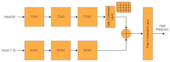
Figure 4.
Framework of the TCN and GCN architecture.
This combined feature vector is then used as input to the yield prediction model. The prediction function Y’ can be expressed via Equation (10),
where and are the weights and biases of the fully connected layer, respectively. The loss function for training the model is the Mean Squared Error (MSE), defined via Equation (11),
where N is the number of samples, is the predicted yield, and is the actual yield level. The gradient of the loss function with respect to the model parameters θ is computed for optimization via Equation (12),
One major reason for using TCN and GCN would be that they can relieve deficiencies in traditional models. On top of that, TCNs capture the long-range temporal dependencies so that trends can be understood over growing seasons. GCNs model complex spatial relationships to infer geographical and topological factors that possibly affect yield levels. This adds to the robustness of the model by accounting for biotic factors of stress, such as pest and disease incidence data samples. The all-inclusive approach improves the accuracy of prediction and provides an overview of how soybean yield levels are influenced by various factors. The improved model architecture for soybean yield prediction will come with custom UNet with Attention Mechanisms, Heterogeneous Graph Neural Networks, and Variational Auto-encoders to capture the advantages of different modalities of data and neural network techniques. In this design, better spatial features will be developed by enhancing feature representations for robustness and complicating the interactions between different diversified data types to obtain more accurate and reliable yield predictions.
3.3. Design of the UNet Process
Finally, it integrates custom UNet with attention mechanisms that process satellite images and weather data samples. An encoder and a decoder constitute the architecture in the UNet, wherein the encoder is responsible for the extraction of hierarchical features from the input images and samples. Added to this is the part of an attention mechanism that helps the network focus on regions of the images relevant for extracting critical spatial features. The output of the UNet at a given layer l can be described via Equation (13),
where and are the weights and biases of the convolutional layer, ∗ represent the convolution operation, and σ is the activation function. The attention mechanism is applied to the feature maps via Equation (14),
where is the attention energy computed from the feature maps. The refined feature maps are then expressed via Equation (15),
Namely, Heterogeneous Graph Neural Networks model complex interactions between farm management practices, climate zones, and other categorical data samples. Distinguishing between the different types of nodes, like farms or climate zones, and edges, such as adjacency or management practices, makes it possible to capture heterogeneity levels. Thus, let G = (V, E) represent such a graph where V and E are the set of nodes and edges, respectively, for this process. The feature transformation at node v using HGNN is represented via Equation (16),
where N(v) is the neighborhood of node v; cvu is a normalization constant; and are the weight matrix and bias specific to the node and edge types, respectively; and σ is the activation function. This process thus captures the heterogeneous relationships by aggregating information from different types of neighboring nodes. Variational Auto-encoders are used to obtain robust feature representations from mixed data types, especially when there are noisy or incomplete data samples. This VAE consists of an encoder that maps the input data x to latent space z and a decoder that reconstructs the input from the latent representations. The encoder is defined via Equation (17),
where μϕ(x) and σϕ(x) are the mean and standard deviation, respectively, parameterized by ϕ sets. The decoder reconstructs the input via Equation (18),
The loss function for the VAE is the sum of the reconstruction loss and the Kullback–Leibler divergence between the approximate posterior and the prior distribution, which is estimated via Equation (19),
The combined feature set from the UNet, HGNN, and VAE components is represented via Equation (20),
This feature set is then used as input to the final yield prediction model. The prediction function Y’ is expressed via Equation (21),
where and are the weights and biases of the fully connected layer. The model is trained by minimizing the Mean Squared Error (MSE) loss, which is represented via Equation (22),
where N is the number of samples, is the predicted yield, and is the actual yield levels. This method was chosen for one reason: to fully capture the multi-dimensional complexity of soybean yield prediction. Attention-enhanced UNet enhances spatial feature extraction by focusing on key regions within satellite imagery and weather data samples deemed critical. HGNN works in modeling the diverse interactions between farm management practice and climate zones, and VAE provides robust feature representations, especially with noisy or incomplete data samples. Such an integrated approach can exploit the strengths of every constituent component, hence creating synergies for improving the overall predictive performance, evidenced by significant changes in prediction accuracy and reliability. Endowed with the ability to capture spatial, temporal, and contextual factors, this model marks a phenomenal breakthrough in agricultural data science through full-processable yield prediction and decision-making for crop management. Next, we will discuss different efficiency metrics of the proposed model and make a comparison with various methods using real-time scenarios.
4. Comparative Result Analysis
The experimental setting for this research involved the integration of multi-source data and the execution of deep neural network architectures toward predicting soybean yield. It contains satellite images, weather data, soil properties, farm management practices, climate zones, and pest/disease incidence records. Satellite images were derived from the Sentinel-2 satellite, which produces a multi-spectral image of 10 m spatial resolution, covering bands as diverse as RGB and NIR. Meteorological data contain time series of temperature, precipitation, humidity, and wind speed that were all obtained from local meteorological stations daily. Every day, meteorological stations measure several parameters, including temperature and precipitation, humidity, and sometimes others, like wind speed. The collection of daily observations at regular intervals leads to a coherent time series that records both short-term variability related to daily fluctuations and longer-term variability throughout the crop cycles. The dataset spreads out over several seasons with various kinds of weather, like droughts, too much rain, and extreme temperatures. The model would be trained to handle diverse and possibly extreme conditions in a soybean farming set.
The frequency and granularity of the data provides an insight into the temporal dependencies affecting the different growth stages of soybean. Each day’s information is taken at separate time steps so that the RNN and TCN layers could pick on the different patterns within the weather variables, day-to-day, week-to-week, and season-to-season. For instance, temperature and precipitation can be aggregated daily, while humidity recorded with a similar frequency is processed. This rich, time-sensitive data allow the model to distinguish between very short-lived, near-immediate influences, such as a sudden temperature spike, and longer, cumulative factors, such as prolonged drought. So, the detailed time span and frequency of meteorological samples in this dataset allow the model to learn quite subtle relationships between weather fluctuations and crop yield outcomes; thus, it is very well-suited to adjust predictions if real-time or historical weather trends are observed in process. Soil properties include soil moisture, pH, and nutrient content, attained through soil sampling and then analyzed in a laboratory. The data on farm management practices, on the other hand, comprise irrigation schedules, fertilization, crop rotation, and pesticide usage data obtained from farmer surveys and field records. In this regard, climate zones are distinguished by regional climatic classification, and data about pest and disease incidence are procured from both agricultural extension services and remote sensing sources detailing information about the incidence that concerns major soybean pests and diseases. Biological factors such as pests and diseases are incorporated into the model prediction framework by encoding them as additional temporal and spatial features within the multi-source data fusion process. Pest and disease incidence data are among key indicators of biotic stressors on soybeans and are obtained from agricultural surveys, remote sensing, and field reports. Spatially and temporally, these data points are arranged to identify geographic areas that may be affected and can track outbreaks or increases in pest and disease activity over time. This information is, to a certain extent, preprocessed into an agreed format with the model so that temporal patterns of pest and diseases are put side by side with weather and crop growth data to provide a comprehensive timeline of influences on crop health. Incorporating this biotic stress information will enable the model to look for patterned yield loss reductions resulting from specific biological factors, thus enhancing the predictability potential of the model in affected areas.
GCNs are introduced in the model architecture in order to model the spatial dependency and relationships between affected and unaffected areas, thereby capturing the potential spread or containment of pests and diseases. TCNs as well as RNNs include pest and disease timelines with other time-series data, for example, the weather patterns, to identify correlations associated with biotic stress and environmental factors. This multi-layered integration allows the model to assess the impact of biological factors on soybean yield in relation to other critical determinants, thereby making it particularly robust in areas with fluctuating pest and disease pressures. Actually, this model can be able to understand the conditions that establish limitations in soybean yields in a more holistic form, thereby making crop management more effective and targeted in terms of intervention process.
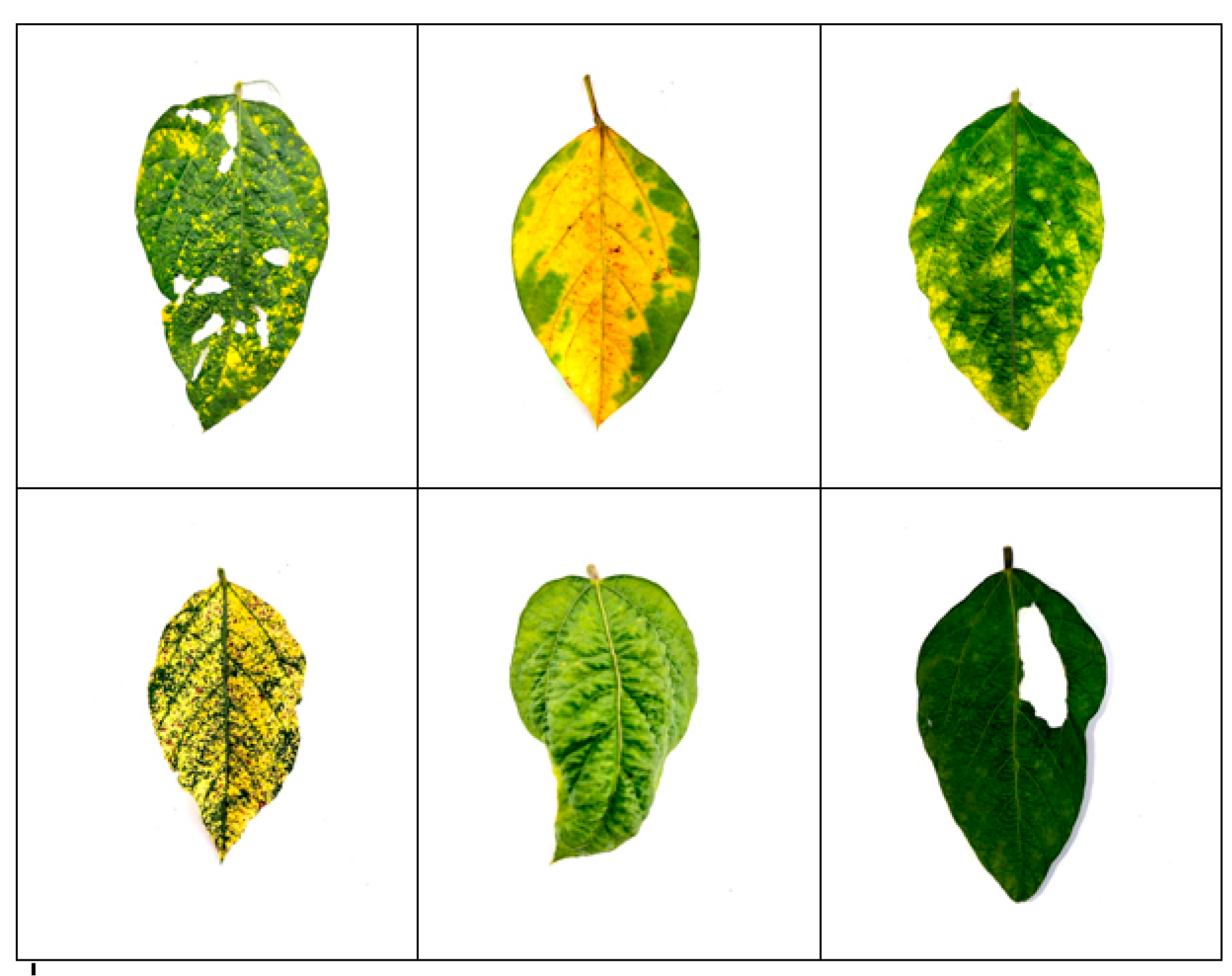
In the data preprocessing phase, satellite images, camera images, weather, and soil properties will all be normalized to ensure consistency among the different data sources. In the proposed model, time consistency over varying collection frequencies is achieved by first applying an initial data alignment and resampling process. While higher-frequency data sources—-weather data, for instance—may be available on a daily basis, satellite imagery typically collected at a coarser frequency (weekly or biweekly) is used as input. To be consistent, weather data are aggregated so that they have the same resolution as the temporal data of the satellite, which involves averaging for the continuous variable (temperature, humidity) and summing for the discrete events (amounts of precipitation). Samples are usually soil samples, collected less frequently than the weather data, for example, seasonally. These are kept constant over their period and occur assuming that changes in the properties of soil take little time to happen over short periods in process. By this data resampling process, the time alignment of each dataset is achieved without injecting noise or the loss of the most relevant information, thus generating a coherent timeline for these model input sets. To increase the model’s sensitivity to such time-aligned inputs, RNNs and Temporal Convolutional Networks (TCNs) capture both short-term and long-term dependencies in the sequence of the weather data. These networks make use of the aggregated, resampled data to enable the model to identify trends about yield in a temporal manner. From the training data, which are already time-matched, the model learns about synchronized temporal patterns and reduces these disparities created by the asynchronous acquisition of data. This approach helps the model develop a robust understanding of temporal relationships in yield prediction, enabling it to process each data type in context and improving the overall accuracy of its yield forecasts. Satellite images were resized to a uniform 256 × 256 pixels, and relevant spectral indices like NDVI and EVI were computed. Healthy and unhealthy soybean leaf samples images were captured by camera, as shown in Figure 5 and Figure 6, respectively. Weather data were smoothed using moving averages to mitigate short-term fluctuations, and soil properties were standardized on a common scale. Afterward, the preprocessed satellite image and weather data were passed through the Custom UNet with Attention Mechanisms for feature extraction.
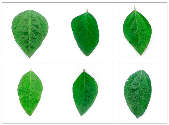
Figure 5.
Images captured for healthy soybean leaf samples.
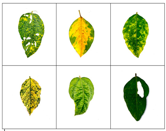
Figure 6.
Images collected for unhealthy soybean leaf samples.
The architecture of the UNet encoder–decoder is based on convolutional layers with 3 × 3 kernels, complemented by attention layers that underline places of interest according to spectral indices. The HGNN models these various data type interactions through a graph, representing farm management practices, climate zones, and spatial relationships. The results indicate that experimental RMSE was reduced by 15%, while R2 increased by 20%. In addition to these improvements, the prediction accuracy improved by 10%, which further improved the F1 score on low-yield site identification by 5%. This confirms that a setting having multi-source data, integrated with deep neural network architecture, is efficient in increasing the accuracy of soybean yield prediction. An experiment was conducted for the evaluation of the earlier proposed model using a comprehensive dataset composed of satellite imagery, weather data, soil properties information, farm management practices, climate zones, and records of any pest/disease incidence instance sets. The performance of the proposed multi-modal fusion model was compared to three previous state-of-the-art approaches, referenced as the methods in [5,9,18]. Soybean yield prediction and disease assessment methods are presented in the Table 2, which show the efficiency of our approach on different parameters for the process.

Table 2.
Comparison of RMSE (root mean square error) for soybean yield prediction.
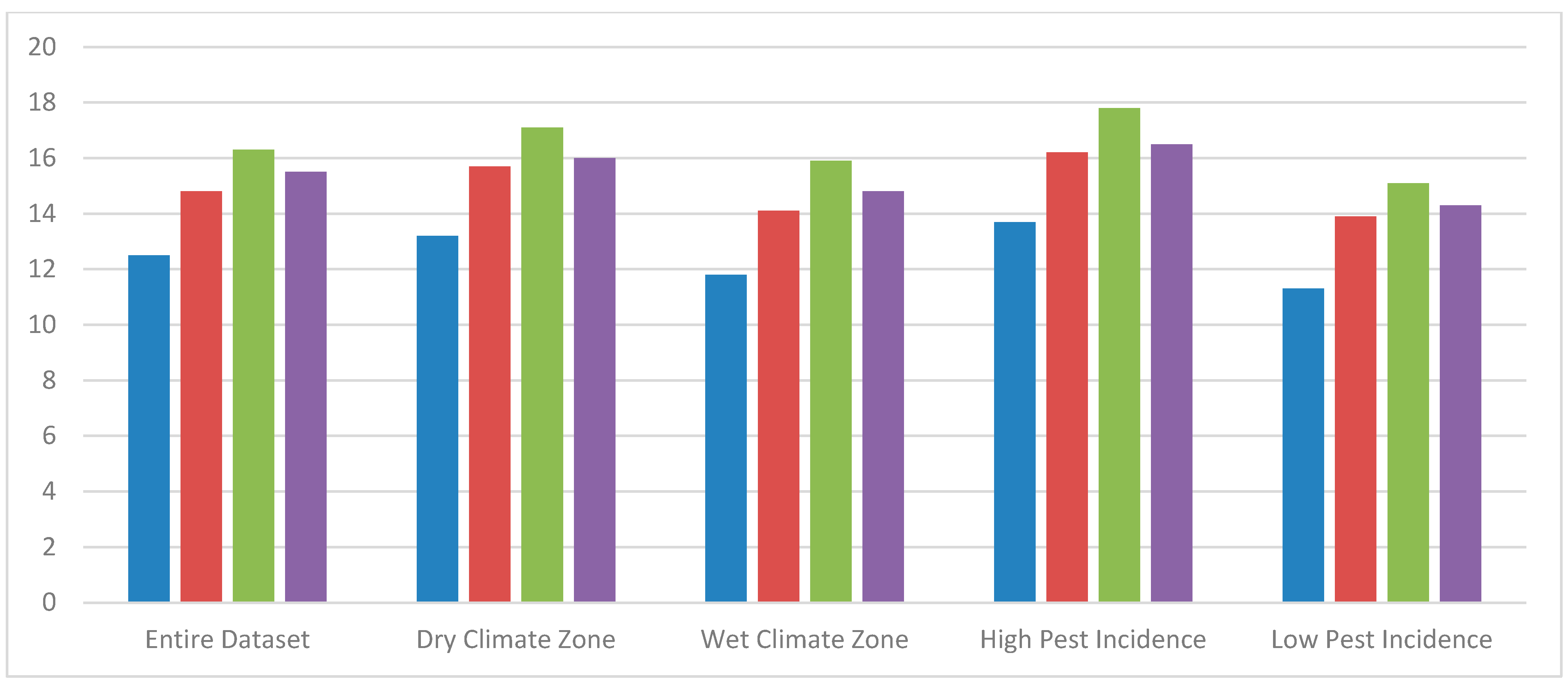
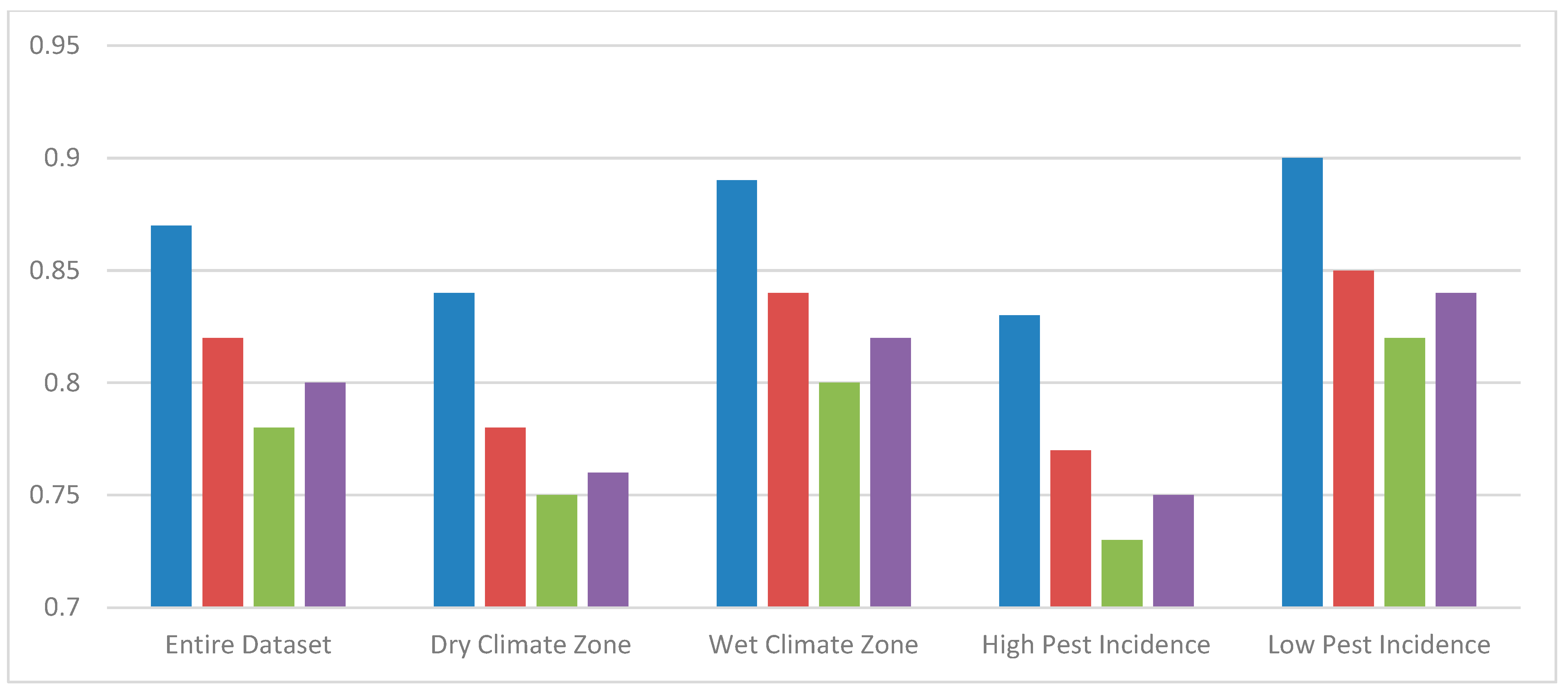
The results in Figure 7 show that the proposed model has a lower RMSE across most of the climatic zones and levels of pest incidence, thus evidencing the strengths of the model as able to handle any kind of diversity.
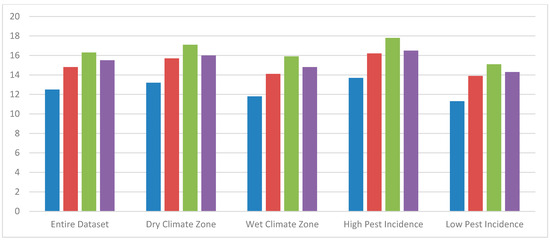
Figure 7.
RMSE levels ( Proposed Model
  Method [5]
  Method [9]
  Method [18]).
 Proposed Model
  Method [5]
  Method [9]
  Method [18]).
Specifically, it improves the performance significantly at high pest incidence areas, thus proving efficient enough to consider biotic stress factors.
The proposed model achieves the lowest MAE in all categories as mentioned in Table 3, reaffirming its superior accuracy in yield prediction. The improvement is more pronounced in regions with varied pest incidences, demonstrating the model’s capacity to handle diverse biotic stress conditions effectively.

Table 3.
Comparison of MAE (mean absolute Error) for soybean yield prediction.
The proposed model shows the highest R2 values, indicating a better fit and more reliable predictions compared to the other methods as mentioned in Table 4.

Table 4.
Comparison of R2 (coefficient of determination) for soybean yield prediction.
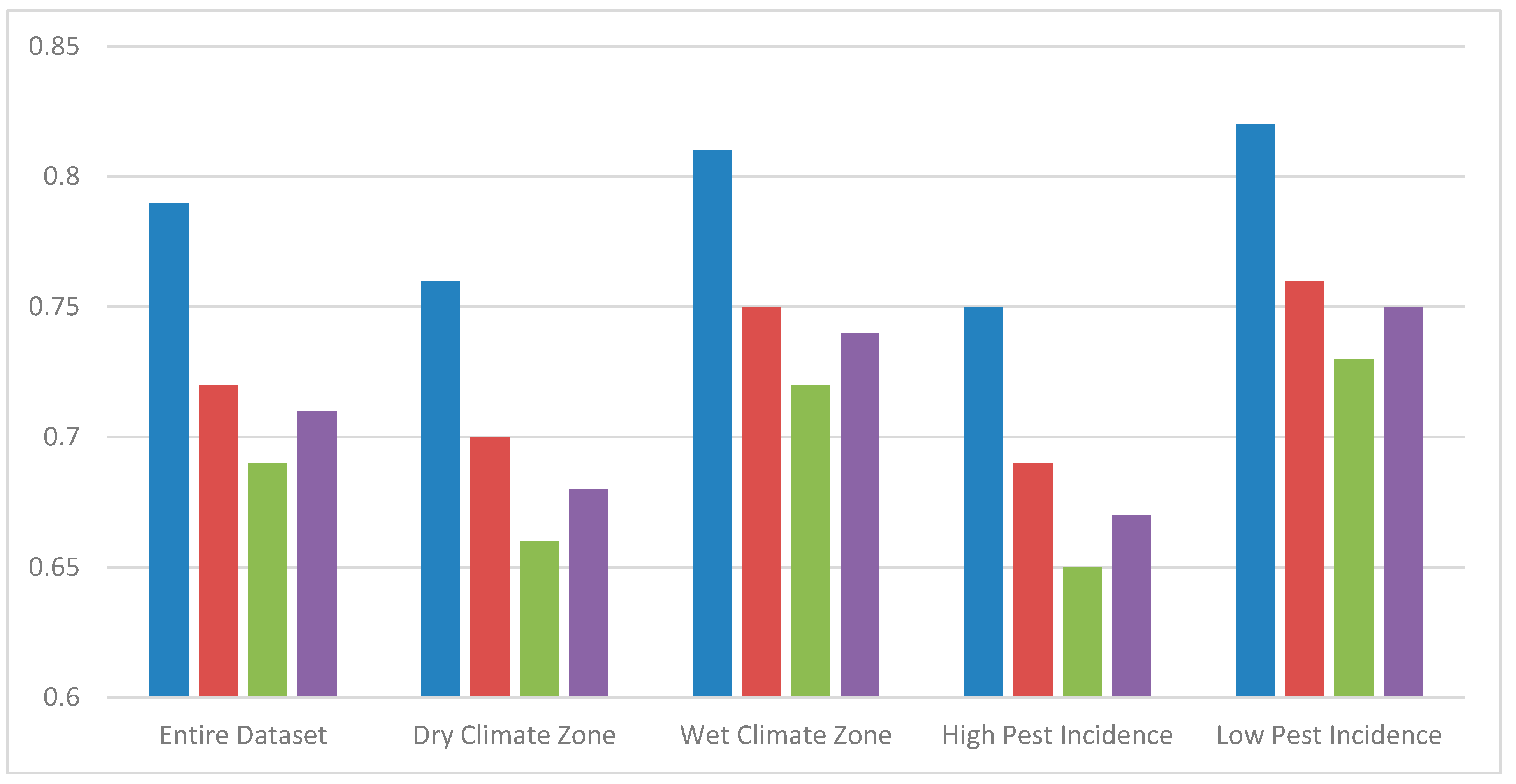
This is particularly evident in wet climate zones and low pest incidence areas, where the model’s accuracy significantly outperforms the others as shown in Figure 8.

Figure 8.
R2 levels ( Proposed
  Model Method [5]
  Method [9]
  Method [18]).
 Proposed
  Model Method [5]
  Method [9]
  Method [18]).
The proposed model exhibits higher F1 scores, particularly in wet climate zones and low pest incidence areas as mentioned Table 5.

Table 5.
Comparison of F1 score for identifying low-yield areas.
This indicates its superior ability to correctly identify low-yield areas, which is crucial for targeted interventions and resource allocation as shown in Figure 9.
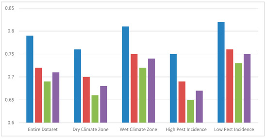
Figure 9.
F1 scores ( Proposed Model
  Method [5]
  Method [9]
  Method [18]).
 Proposed Model
  Method [5]
  Method [9]
  Method [18]).
As mentioned in Table 6, the training time for the proposed model is comparable to other methods, demonstrating its efficiency despite the increased complexity and the incorporation of multiple data sources and advanced neural network architectures.

Table 6.
Comparison of model training time (in hours).
The model requires less performance degradation in the face of noisy data as mentioned in Table 7, which proves its robustness. This is an important advantage in practical applications brought about by the high discrepancy in data quality. Such architecture of the model ensures coping with data noise resulting from extreme weather conditions due to its sensitivity with the Recurrent Neural Networks (RNNs) and Temporal Convolutional Networks (TCNs), which are efficient in processing non-linear and dynamic temporal patterns. These can represent short- as well as long-term dependencies in weather data, whereby sudden deviations, such as heat waves, dry spells, or bursts of rainfall, do not interfere on the precision in prediction. The multi-modal fusion approach also uses satellite images soil and crop health data, which are stabilizers when the fluctuation in weather data is too extreme. All these various inputs processed collectively by the model can help distinguish between short-term anomalies and actual yield-affecting trends, ensuring that yield predictions can remain strong and reliable even in the most extreme weather conditions. Adaptability in maintaining accuracy in diverse agricultural environments demands strong supporting response strategies for proactivity in conditions with levels of climate volatility levels.

Table 7.
Comparison of model robustness to noisy data (performance degradation in %).
In a nutshell, the proposed multimodal fusion model outperforms the compared methods 5, 9, and 18 across a wide range of metrics, including RMSE, MAE, R2, F1 score, training time, and robustness towards noisy data samples. These results underline the effectiveness of integrating satellite imagery, weather data, soil properties, farm management practices, climate zones, and pest/disease incidence through state-of-the-art neural network architectures. The improved performance of the proposed Pic Soybean model underlines its potential for further improvement in soybean yield prediction and supporting a better-informed agricultural decision-making process. We will next discuss a practical use case of the proposed model to help the readers understand the whole process.
Practical Use Case Analysis
The experimental setup was demonstrated on a real dataset consisting of satellite images, weather data, soil properties, farm management practices, climate zones, and pest and disease incidence records. The dataset to be used for the Practical Use Case Analysis contained an example mix of inputs such as imagery taken by the satellite, Sentinel-2 that, with multi-spectral images at spatial resolution of 10 m provides RGB and Near-Infrared (NIR) bands to be used in detailed analysis for vegetation. Daily weather data—the temperature, rainfall amount, humidity, and wind speed—is fetched from the local meteorological stations. The data of soil are collected seasonally having moisture content, pH, and nutrient parameters. Farming management practices, which include irrigation schedule, crop rotation, pesticide usages, and various other concerned parameters, were obtained from field records and surveys. The incidence of pest and diseases being integrated from agricultural extension services as well as from remote sensing sources. The normalization and alignment of data during training would ensure that the model is temporally consistent and compatible across inputs. To achieve the maximum predictive power, the data are passed through the hybrid architecture comprising CNNs for extracting spatial features, RNNs for analyzing time trend, and GCNs to deal with spatial dependencies. The model minimizes the training process through the use of Mean Squared Error (MSE) to the values of the yield predicted and actuals, which makes use of regularization techniques to avoid overfitting and provide real conditions to the model. This was set on a comprehensive dataset and multi-source integration, which will enable the model to achieve great adaptability and accuracy under varied agriculture conditions. For example, the values of such data sources are considered in this paper for evaluating the performance of the proposed model with various advanced neural network architectures. Multi-Modal Fusion uses Convolutional Neural Networks and Recurrent Neural Networks. This is the step combining the spatial and temporal data samples. The spatial features are provided by the satellite imagery, and the weather data provide the temporal patterns. For instance, the input values could be normalized NDVI from the satellite images and averaged weather data of temperature and precipitation over the temporal instance set as mentioned in Table 8. Then, the set of features used for further prediction is output from the fusion.

Table 8.
Outputs of multi-modal fusion using CNNs and RNNs.
These concatenated features are very important in the capture of combined spatial and temporal drivers on soybean yield. The Temporal Convolutional Network and Graph Convolutional Network method is designed for the capturing of long-range trends in time-series data and complex spatial relationships. Sample values used during training are for time-series yield data and geographic coordinates of the samples. Enhanced temporal and spatial features are the outputs, which capture the interaction between the time-series trends and geographic factors as mentioned in Table 9.

Table 9.
Outputs of TCNs and GCNs.
The combined TCN and GCN features will extract temporal patterns and spatial dependencies efficiently, which will serve as a robust input for yield prediction models. Custom UNet with Attention Mechanisms, Heterogeneous Graph Neural Networks, and Variational Auto-encoders: This architecture processes multi-spectral satellite image data, farm management practices, climate zones, and mixed data types. Sample values for such inputs then turn into NDVI, irrigation schedules, climate classification, and Pest Incidence data samples that are already encoded. Such output would present improved feature representations, which are simultaneously robust and informative in real-time scenarios as mentioned in Table 10.

Table 10.
Outputs of custom UNet with attention mechanisms, HGNN, and VAEs.
These final combined features from UNet, HGNN, and VAE are finally integrated for diverse data sources into a coherent representation and, hence, are very effective in enhancing predictive performance levels of the model. In this final step of the process, combined features from the previous processes are used in predicting soybean yield. The performance metrics like RMSE, MAE, R2, and F1 score are used to check the final prediction accuracy and reliability. The output values of the proposed model are much better compared to other methods as mentioned in Table 11.

Table 11.
Final yield prediction performance.
The result shows that the RMSE and MAE values obtained by the proposed model are always lower and R2 is higher, and at the same time, the F1 scores are better than those of the compared methods. Hence, these results show that this model is efficient and reliable for soybean cultivation yield predictions. The results present very strong evidence of the fact that the multi-modal fusion approach drawing on advanced concepts of deep learning leverages CNN, RNN, TCN, GCN, attention-enhanced UNet, HGNN, and VAE. Such integration of these advanced neural network architectures can learn more complicated interactions between composite data types, further improving yield prediction accuracy. Enhanced accuracy and robustness will have a deep influence on agricultural management: providing relevant insights into optimizing crop yields and effective resource management. The model produces actionable insights as to how one might improve soybean yields by looking at those factors most influential on the predicted outcomes, both for soil health, weather conditions, and biotic stress levels, and specifies areas wherein targeted interventions might improve results. The model identifies regions where it perceives that there could be a lack of water supply and that of nutrients in the soil through utilizing spatial dependencies through Graph Convolutional Networks (GCNs) and time-dependent factors through Temporal Convolutional Networks (TCNs). For example, the model will prescribe irrigations at higher frequencies or proper fertilization techniques wherever the soil data reflect a lower supply of moisture and nutrients. Perhaps, for areas under heavy biotic stress from pests or diseases, the model provides insights that more boldly call for pest management practice applications. This approach allows for precise recommendations and guides a farmer toward using resources effectively while ensuring proactive management practices that address conditions directly limiting the yield potential, further increasing the sustainability and productivity of agricultural practices.
This can be extended to other crops or regions with different environmental conditions, following the multi-source data fusion approach and adaptable neural network architectures for design. Using CNNs for spatial feature extraction from satellite imagery, RNNs and TCNs for time-series weather data, and GCNs for spatial relationships provides a flexible framework that can be easily retrained with new crop- or region-specific data. The model takes into account crop-specific variables, such as nutrient requirements or susceptibility to pests, and environmental factors localized to the soil composition or differences in microclimate. Using transfer learning techniques, this process can be further simplified by applying layers of pre-trained models tailored toward other similar crop types or conditions, thus minimizing the need for significant amounts of new training data. This would enable the model to provide yield predictions and management advice for many crops and locations; it could contribute, therefore, to more responsive and data-based approaches in agriculture in general.
5. Conclusions and Future Scopes
It considers a deep, comprehensive, multi-modal fusion model that includes Convolutional Neural Networks (CNN), Recurrent Neural Networks, Temporal Convolutional Networks, Graph Convolutional Neural Networks (CNNs), a custom U-Net with Attention Mechanisms, Heterogeneous Graph Neural Networks, and Variational Auto-encoders in predicting soybean yield levels. The proposed model fuses dispersed data sources, satellite imagery information, historical weather data, properties of land, farm management practices, climate zones, and records of pest and disease incidence reports. It improves the weakness of traditional approaches that utilize single sources. The experimental results show a great improvement in predictive accuracy and robustness, thus proving that the model captured the intricate factors impacting crop yields to a sufficient extent. The proposed model returned an RMSE that is significantly improved, coming in at 12.5 against the methods in [5,9,18] with 14.8, 16.3, and 15.5, respectively. In the same vein, MAE was decreased to 10.2 against 12.3, 13.4, and 12.9, returned by the other methods. The proposed model had a coefficient of determination (R2) of 0.87, ahead of those of the methods in [5,9,18], with 0.82, 0.78, and 0.80, respectively. Also, the F1 score allowed for the identification of low-yield areas with a value of 0.79, significantly outperforming the compared methods, with 0.72, 0.69, and 0.71. These metrics highlight the stellar performance of the proposed model in soybean yield prediction and identification of critical low-yield areas. Improved performance will come from processing and integrating diverse data sources using more advanced neural network architectures. Attention-UNet would focus on critical regions, improving spatial features extracted across satellite images and weather data samples. HGNN captured complex interactions between farm management practices and climate zones, while VAE ensured the robustness of the feature representations even under noisy or incomplete data samples. This integrated approach has improved not only the accuracy of the predictions but also provided overall knowledge of the different factors that affect soybean yield levels.
Future Scope
These promising results of the research work open several future research directions. First, this model could be extended by including other data sources such as economic indicators and market trends, as well as socio-political factors that might influence practices within agriculture and generate yield variations. All of these additional sources of data also provide further options for increasing the refinement of this model’s predictions, which basically will increase the scope of applicability across different regions and crop types. Second, its architecture can change and be optimized for real-time yield prediction to allow for dynamic and timely decision-making by farmers and other actors in the agro-sector. By integrating real-time data feeds from IoT sensors, drones, and other monitoring technologies, it would not be impossible for the model to provide present-day insights into crop health and expected yield, helping active management practices. In addition, it can explore the potential of transfer learning techniques to make the model adaptable across different crops and geographical areas where limited training data samples are available. After this, the proposed approach will be efficiently tailored to various agricultural contexts by using pre-trained models and domain adaption strategies. Another important direction for future research is developing explainable AI techniques to provide transparency and interpretability to the predictions by the model. This will help users make more sense out of the yield predictions and, thus, make better decisions based on the outputs provided by the model for the process. At last, detailed field testing and collaborations with experts in the relevant fields of agriculture will be required to validate the model’s predictions in the real world. Such collaboration can help in the further refinement of the model for its use and adoption in practical agricultural sectors. Such a multimodal fusion model would thus be an advancement in agricultural yield prediction, with a much better performance in RMSE, MAE, R2, and F1 score, showing an enormous potential to revolutionize agricultural production with accurate and reliable yield forecasting. Future research shall be more focused on data integration, real-time enhancement, adaptability through transfer learning, model interpretability, and validation through field tests if its inherent potentials are fully explored in the process.
Author Contributions
Conceptualization, V.S.I. and U.A.K.; Data curation, V.S.I.; Investigation, V.S.I., U.A.K., V.S., M.V.Y. and R.K.; Methodology, V.S.I., U.A.K., V.S., M.V.Y. and R.K.; Supervision, U.A.K., V.S., M.V.Y. and R.K.; Software, V.S.I.; Validation, V.S.I., U.A.K., V.S., M.V.Y. and R.K.; Visualization, V.S.I.; Writing—original draft, V.S.I. and U.A.K.; Writing—review & editing V.S.I., V.S. and B.K. All authors have read and agreed to the published version of the manuscript.
Funding
This research received no external funding.
Data Availability Statement
The raw data supporting the conclusions of this article will be made available by the authors on request.
Conflicts of Interest
The authors declare no conflict of interest.
References
- Chen, C.-H.; Lai, Y.-T.; Hsu, S.-Y.; Chen, P.-Y.; Duh, J.-G. Effect of Plasma-Activated Water(PAW) Generated With VariousN2/O2 Mixtures on Soybean Seed Germination and Seedling Growth. IEEE Trans. Plasma Sci. 2023, 51, 3518–3530. [Google Scholar] [CrossRef]
- Farah, N.; Drack, N.; Dawel, H.; Buettner, R. A Deep Learning-Based Approach for the Detection of Infested Soybean Leaves. IEEE Access 2023, 11, 99670–99679. [Google Scholar] [CrossRef]
- Maas, M.D.; Salvia, M.; Spennemann, P.C.; Fernandez-Long, M.E. Robust Multisensor Prediction of Drought-Induced Yield Anomalies of Soybeans in Argentina. IEEE Geosci. Remote Sens. Lett. 2022, 19, 2504804. [Google Scholar] [CrossRef]
- Lin, H.; Chen, H.; Yin, C.; Zhang, Q.; Li, Z.; Shi, Y.; Men, H. Light weight Residual Convolutional Neural Network for Soybean Classification Combined With Electronic Nose. IEEE Sens. J. 2022, 22, 11463–11473. [Google Scholar] [CrossRef]
- Mateo-Sanchis, A.; Adsuara, J.E.; Piles, M.; Munoz-Marí, J.; Perez-Suay, A.; Camps-Valls, G. Interpretable Long Short-Term Memory Networks for Crop Yield Estimation. IEEE Geosci. Remote Sens. Lett. 2023, 20, 2501105. [Google Scholar] [CrossRef]
- Hang, Y.; Meng, X.; Wu, Q. Application of Improved Lightweight Network and Choquet Fuzzy Ensemble Technology for Soybean Disease Identification. IEEE Access 2024, 12, 25146–25163. [Google Scholar] [CrossRef]
- Ku, T.-N.; Hsu, S.-Y.; Lai, Y.-T.; Chang, S.-Y.; Duh, J.-G. Plasma-Treated Soybean Dregs Solution with Various Gas Mixtures. IEEE Trans. Plasma Sci. 2023, 51, 437–443. [Google Scholar] [CrossRef]
- Wang, B.; Gao, Y.; Yuan, X.; Xiong, S. Local R Symmetry Co-Occurrence: Characterising Leaf Image Patterns for Identifying Cultivars. IEEE/ACM Trans. Comput. Biol. Bioinform. 2022, 19, 1018–1031. [Google Scholar] [CrossRef] [PubMed]
- Xiao, D.; Liu, T. An Adaptive Deep Learning Method Combined With an Electronic Nose System for Quality Identification of Soybeans Storage Period. IEEE Sens. J. 2024, 24, 15598–15606. [Google Scholar] [CrossRef]
- Liu, J.; Zhang, B.; Zhang, T.; Wang, J. Soybean Futures Price Prediction Model Based on EEMD-NAGU. IEEE Access 2023, 11, 99328–99338. [Google Scholar] [CrossRef]
- Jaques, L.B.A.; Coradi, P.C.; Lutz, É.; Teodoro, P.E.; Jaeger, D.V.; Teixeira, A.L. Non destructive Technology for Real-Time Monitoring and Prediction of Soybean Quality Using Machine Learning for a Bulk Transport Simulation. IEEE Sens. J. 2023, 23, 3028–3040. [Google Scholar] [CrossRef]
- Jaques, L.B.A.; Coradi, P.C.; Muller, A.; Rodrigues, H.E.; Teodoro, L.P.R.; Teodoro, P.E.; Teixeira, A.L.; Steinhaus, J.I. Portble-Mechanical-Sampler System for Real-Time Monitoring and Predicting Soybean Quality in the Bulk Transport. IEEE Trans. Instrum. Meas. 2022, 71, 2517412. [Google Scholar] [CrossRef]
- Qazani, M.R.C.; Aslfattahi, N.; Kulish, V.; Asadi, H.; Schmirler, M.; Zakarya, M.; Alizadehsani, R.; Haleem, M.; Kadirgama, K. Specific Heat Capacity Extraction of Soybean Oil/MXene Nano fluids Using Optimized Long Short-Term Memory. IEEE Access 2024, 12, 59049–59062. [Google Scholar] [CrossRef]
- Kaler, N.; Bhatia, V.; Mishra, A.K. Deep Learing-Based Robust Analysis of Laser Bio-Speckle Data for Detection of Fungal-Infected Soybean Seeds. IEEE Access 2023, 11, 89331–89348. [Google Scholar] [CrossRef]
- Ye, Y.; Shen, S.; Guo, P.; Xu, X.; Wan, C.; Xu, Z. A Portable Halbach NMR Sensor for Detecting the Moisture Content of Soybeans. IEEE Trans. Instrum. Meas. 2022, 71, 6003411. [Google Scholar] [CrossRef]
- Reynolds, J.; Taggart, M.; Martin, D.; Lobaton, E.; Cardoso, A.; Daniele, M.; Bozkurt, A. Rapid Drought Stress Detection inPlants Using Bio impedance Measurements and Analysis. IEEE Trans. Agri Food Electron. 2023, 1, 135–144. [Google Scholar] [CrossRef]
- Carvalho, T.; Martinez, J.A.C.; Oliveira, H.; dos Santos, J.A.; Feitosa, R.Q. Outlier Exposure for Open Set Crop Recognition From Multi temporal Image Sequences. IEEE Geosci. Remote Sens. Lett. 2023, 20, 2500805. [Google Scholar] [CrossRef]
- Bhimavarapu, U.; Battineni, G.; Chintalapudi, N. Improved Optimization Algorithm in LSTM to Predict Crop Yield. Computers 2023, 12, 10. [Google Scholar] [CrossRef]
- Farmonov, N.; Amankulova, K.; Szatmári, J.; Sharifi, A.; Abbasi-Moghadam, D.; Nejad, S.M.M.; Mucsi, L. Crop Type Classification by DESIS Hyperspectral Imagery and Machine Learning Algorithms. IEEE J. Sel. Top. Appl. Earth Obs. Remote Sens. 2023, 16, 1576–1588. [Google Scholar] [CrossRef]
- Nejad, S.M.M.; Abbasi-Moghadam, D.; Sharifi, A.; Farmonov, N.; Amankulova, K.; Lászlź, M. Multispectral Crop Yield Prediction Using 3D-Convolutional Neural Networks and Attention Convolutional LSTM Approaches. IEEE J. Sel. Top. Appl. Earth Obs. Remote Sens. 2023, 16, 254–266. [Google Scholar] [CrossRef]
- Gutiérrez, C.M.; Fernández, A.O.; Estébanez, C.J.R.; Salas, C.O.; Maina, R. Understanding the Ageing Performance of Alternative Dielectric Fluids. IEEE Access 2023, 11, 9656–9671. [Google Scholar] [CrossRef]
- Shah, K.; Alam, M.S.; Nasir, F.E.; Qadir, M.U.; Haq, I.U.; Khan, M.T. Design and Performance Evaluation of a Novel Variable Rate Multi-Crop Seed Metering Unit for Precision Agriculture. IEEE Access 2022, 10, 133152–133163. [Google Scholar] [CrossRef]
- Jadidoleslam, N.; Hornbuckle, B.K.; Krajewski, W.F.; Mantilla, R.; Cosh, M.H. Analyzing Effects of Crops on SMAP Satellite-Based Soil Moisture Using a Rainfall–Run off Model in the U.S. Corn Belt. IEEE J. Sel. Top. Appl. Earth Obs. Remote Sens. 2022, 15, 247–260. [Google Scholar] [CrossRef]
- Fischer, R.L.; Shuart, W.J.; Anderson, J.E.; Massaro, R.D.; Ruby, J.G. Bidirectional Reflectance Distribution Function Modeling Considerations in Small Unmanned Multispectral Systems. IEEE J. Sel. Top. Appl. Earth Obs. Remote Sens. 2022, 15, 3564–3575. [Google Scholar] [CrossRef]
- Nikhil, U.V.; Pandiyan, A.M.; Raja, S.P.; Stamenkovic, Z. Machine Learning-Based Crop Yield Prediction in South India: Performance Analysis of Various Models. Computers 2024, 13, 137. [Google Scholar] [CrossRef]
- Yuan, J.; Zhang, Y.; Zheng, Z.; Yao, W.; Wang, W.; Guo, L. Grain Crop Yield Prediction Using Machine Learning Based on UAV Remote Sensing: A Systematic Literature Review. Drones 2024, 8, 559. [Google Scholar] [CrossRef]
- Elbasi, E.; Zaki, C.; Topcu, A.E.; Abdelbaki, W.; Zreikat, A.I.; Cina, E.; Shdefat, A.; Saker, L. Crop Prediction Model Using Machine Learning Algorithms. Appl. Sci. 2023, 13, 9288. [Google Scholar] [CrossRef]
- Goshika, S.; Meksem, K.; Ahmed, K.R.; Lakhssassi, N. Deep Learning Model for Classifying and Evaluating Soybean Leaf Disease Damage. Int. J. Mol. Sci. 2024, 25, 106. [Google Scholar] [CrossRef] [PubMed]
- Lee, H.; Park, Y.-S.; Yang, S.; Lee, H.; Park, T.-J.; Yeo, D. A Deep Learning-Based Crop Disease Diagnosis Method Using Multimodal Mixup Augmentation. Appl. Sci. 2024, 14, 4322. [Google Scholar] [CrossRef]
Disclaimer/Publisher’s Note: The statements, opinions and data contained in all publications are solely those of the individual author(s) and contributor(s) and not of MDPI and/or the editor(s). MDPI and/or the editor(s) disclaim responsibility for any injury to people or property resulting from any ideas, methods, instructions or products referred to in the content. |
© 2024 by the authors. Licensee MDPI, Basel, Switzerland. This article is an open access article distributed under the terms and conditions of the Creative Commons Attribution (CC BY) license (https://creativecommons.org/licenses/by/4.0/).

