1. Introduction
The study of structural dynamics is essential for understanding and evaluating the performance of any engineering structure. Most structures vibrate. In operation, all machines, vehicles and buildings are subjected to dynamic forces that cause vibrations. Very often, the vibrations have to be investigated because they may cause an immediate problem. Whatever the reason, we need to quantify the structural response in some way, so that its implication on factors such as performance and fatigue can be evaluated. The frequency response function (FRF) will then be considered. These structures may have a uniform geometry or a periodic one. The frequency response function has acquired much consideration for high frequencies, since at small values, the system can be analyzed statically. Getting this function for the structures and system mentioned under a high range of angular frequencies will lead to a large amount of computation time, since solving for the displacement vector requires inversing the dynamic stiffness matrix at each angular frequency. As the number of substructures, also called cells, increases the computational cost increases. Hence, the approach emphasized in this research presents a solution for this time issue.
Various methods were inspected to determine the frequency response for one-dimensional structures and their behavior as assembled for a two-dimensional element as a truss or frame. Original numerical approaches were done by Dong and Aalami [
1,
2] to estimate the deformations on each point on the cross-section by finite element analysis (conventional FEM).
One approach for structural analysis is the spectral finite element method (SFEM) that was mainly used by Finnveden [
3,
4]. It considers general uniform structures with complex cross-sections and handles all types of boundary conditions. The displacements in the cross-section are described by the finite element method (FEM), while ordinary differential equations for 2D structures will express the variation along the axis of symmetry (
x-axis) with a solution of the form
, where
y and
z are cross-sectional coordinates. A similar approach as SFEM called the dynamic stiffness method (DSM) is notably efficient for the study of excited structures under high frequencies [
5]. It provides an economical solution with a much higher accuracy, since it divides the member into distinct elements. Both methods include similar steps till the extent of obtaining the dynamic stiffness matrix. DSM defines a relationship between the nodal displacement and forces of the element using shape functions, in order to derive the dynamic stiffness matrix; whereas the SFEM uses the virtual work method to obtain the stiffness matrix, and the dynamic matrix will have a more laborious presentation, being a function of the wave number. Structures made of plates and shells were examined by the SFEM approach by Nilsson [
6]. Birgersson [
7,
8,
9] studied plane wave and fluid structure interaction. Gry and Gavric [
10,
11] applied similar approaches for the detection of wave propagation on rails, where they calculated the relative dispersion relations. Similar techniques were interpreted by Bartoli and Marzani [
12,
13] for the purpose of computing the dispersion relations for damped structures of arbitrary cross-sections and with symmetric elements.
Duhamel et al. [
14] established a combined method between wave and finite element approaches for investigating periodic structures; it has an advantage over the SFEM by its ease of operations for complex geometries and scattered materials. Lee et al. [
15] utilized a compounded method using finite element and boundary element (FEBE) methods for studying periodic structures meshed non-periodically.
Reduced order models (ROMs) are mainly mathematically-inexpensive methods for solving complex and large-scale dynamic problems by decreasing the model’s degrees of freedom. It gathers the system’s responses under excitations, providing near real-life analysis, however with low accuracy. ROM was applied on mistuned bladed disks by Castanier et al. [
16] for capturing localized modes and producing low order models with modest memory storage; it calculated relatively acceptable results in comparison with FEM. The method was later improved by employing the Craig–Bampton component mode synthesis (CMS), which is an ROM-based technique yielding better mode accuracy; it required that at least one subspace iteration is executed (Bathe et al. [
17]). CMS was then applied by Zhou et al. [
18] on dynamics analysis using non-uniform rational B-spline (NURBS) finite elements to generate appropriate constructions of interfaced substructures. The method obtained a complete structural model consistent with the original model.
Duhamel [
19,
20] analyzed the frequency response by the recursive method (RM), on waveguide structures, as beams, plates and tires. The beam was divided into two substructures. As the division number increases, a higher accuracy in the frequency response is obtained. He also studied some plates excited in the mid
x and
y positions. A simply supported plate is meshed, and then, its mass and stiffness matrices are extracted from ABAQUS and then inserted in MATLAB to obtain the frequency response using the method studied. A similar method aiming to reduce the number of degrees of freedom under zero forces called the Guyan method is commonly used; however, it had been employed mainly for static analysis. Further, it neglects the inertia at the omitted DOF, hence being obsolete for structures of high mass to stiffness ratios [
21].
The paper provides a computational solving method for periodic structures that cannot be designed as waveguides, where the recursive method is studied for its efficiency. The recursive method tends to ease the study of finite element analysis for complex structures. It is a computational method that computes the global dynamic stiffness matrix by products and inverses of matrices, resulting with the same dimension as that of one cell. For a complex cross-section, the structure is sectioned and modeled in the conventional finite element software and then post-processed in MATLAB. RM tends to eliminate any degrees of freedom (DOF) on the nodes that are not under study. Thus, a structure of two elements can be examined as one, on account of omitting the DOF at the boundaries between two consecutive cells, if there were no internal loads.
Two applications were examined under the illustrated method. The first application is where the RM is applied on 1D bar structures and demonstrating their manner as assembled in a crane under harmonic and seismic loadings. The crane will be dealt with as a truss. A real-life example will be considered, with a conservative number of elements. For the second application, the RM will be applied on a building modeled as a frame. The seismic load will be designed as harmonic displacement at its base end. The truss and the frame are considered as 2D periodic structures.
Modal analysis is used to assess the dynamic properties of a structure by assessing the natural frequencies and their corresponding mode shapes. It was employed to determine the range of frequencies to be examined. FEM works on the full modes when computing the FRF, while RM will only work on the modes that include the studied nodes. For example, in the presented study, the structure has no internal nodes for examination; hence, RM will consider the first mode only with the two end nodes. Using the recursive method, a few computations are needed for finding a close response compared to the number of computations used in the finite element analysis.
2. Recursive Method
2.1. Review
The recursive method is used to calculate the forced response of various types of structures, which might lead to a high consumption of computation. This method is used to compute the general dynamic stiffness matrix with a much lower amount of computational time. Generally, the recursive method is a purely computational method, which computes the global dynamic stiffness matrix by products and inverses of matrices with the same dimensions as the dynamic stiffness matrix of a cell.
For a complex cross-section, the structure is sectioned and modeled in the conventional finite element software (ANSYS). Then, the mass, stiffness and damping matrices are extracted from ANSYS.
These matrices will be post-processed to give the dynamic stiffness matrix of the section under study, after which, the global dynamic stiffness matrix of the whole structure will be figured from the recursive method. It will be obtained by means of products and inverses of the matrices with the dimension equal to that of the dynamic stiffness matrix of the section. This method tends to eliminate any degrees of freedom (DOF) on the nodes that are not under study. Thus, a structure of two elements can be examined as one, on account of omitting the DOF at the boundaries between two consecutive cells, if there were no internal loads. In general, this method is applicable and effective when the structure is not under a large number of forces.
The periodic structure that is divided into
N cells is considered. The problem studied is under a point force excitation, having a response
. Following is a demonstration for the recursive method, numerically [
14].
2.2. Behavior of One Cell
First, consider a one-cell element. The discrete dynamic stiffness matrix of a cell for a time-dependent
is given by:
where
,
is the angular frequency,
is the stiffness matrix,
is the damping matrix,
is the mass matrix,
is the displacement vector and
is the loading vector.
Thus, the dynamic stiffness matrix is:
Decomposing the degrees of freedom into the boundary (
B) and interior (
I), the resulting dynamic equation is:
Then, eliminate the second row of Equation (3):
The first row in Equation (3) will be:
Thus, boundary conditions are only considered in the study. These conditions can be decomposed into left (L) and right (R) for the relative nodes.
Equation (5) becomes:
where
is the dynamic stiffness matrix of a single cell.
Since matrices , and are symmetric, matrix will also be symmetric.
2.3. Behavior of Two Cells
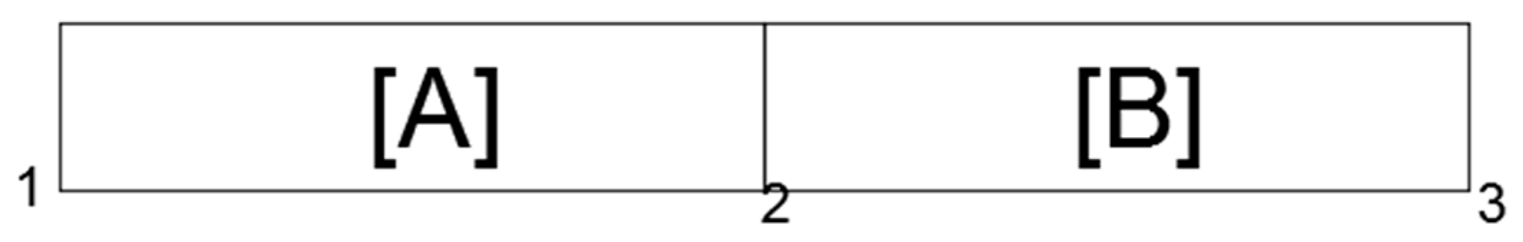
For the assembly of two cells, consider the dynamic stiffness matrices
A and
B for Cell 1 and Cell 2, respectively, as shown in
Figure 1. The dynamic stiffness matrix is now denoted with
, which relates the DOF between the two sides (left and right). The dynamic stiffness matrix of the structure is calculated using:
since the interior side is taken with free loading
. Thus, solving for the second row in the matrix:
The global dynamic stiffness matrix will then be:
where
is the dynamic stiffness matrix of the two cells’ structure.
Since matrices
and
are symmetric, matrix
will also be symmetric. Therefore, we can write:
2.4. General Case
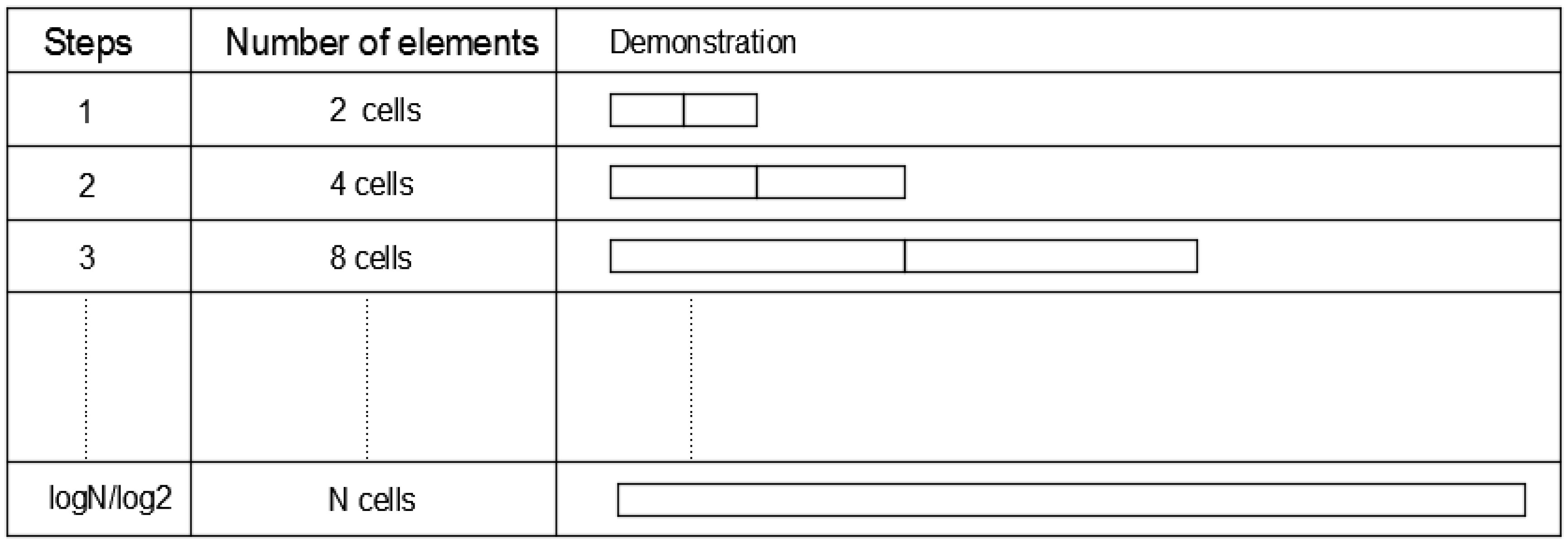
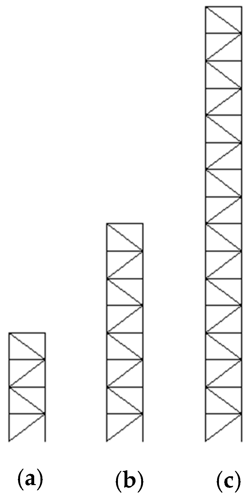
Consider now a general case of a structure made of
N cells, where it is under no load at its internal nodes. Denote its total dynamic stiffness matrix as
. Note that the structure is periodic and is isotropic. Firstly, consider a structure with identical cells; omit the internal degrees of freedom that are under no load. As stated in the foregoing method, the element of two cells is subsequently modeled as one cell. Hence, the current one-cell element will be assembled with a one-cell element that was previously a two-cell element. Proceeding with the
N-cell structure, the outcome is a one-cell element that holds the nodes that are of interest for the assessment. For no restriction on the number of cells, the procedure is computed for
steps. This accustomed number of steps will have a high effectiveness on saving the number of computations, when comparing with the conventional finite element analysis; since it is no longer required for the global assembly of the whole structure. The complete analysis is reviewed in
Figure 2.
In case the number of cells was not as a power of two, a binary representation will be used to model the system. For example, for N number of cells where N is not equal to a number with a power of two, it can be written in binary representation as .
The system is solved as follows:
Calculate the dynamic stiffness matrix for a structure of eight cells, decomposing them into four of two cells each.
The studied structure is then assembled with a structure of two cells, studied previously.
The resulting matrix is assembled with a structure of one cell.
This approach can be resumed by:
This method provides an easy approach for the computations of a structure with a large number of cells under harmonic vibrations. After applying the force and displacement boundary conditions, the response for the node subjected to forced vibrations is studied and detected for the frequency response function.
3. Applications
Periodic structures were examined in this paper. For the first application, 1D bar structures are assembled in a crane. Excitation and seismic loading will be examined on cranes, where it will be dealt with as a truss. On the other hand, the application of the recursive method will be on 2D frame, where a harmonic displacement is loaded at its base nodes (model of seismic load). The frame is considered as a 2D periodic structure.
After computing the FRF conventionally (using harmonic analysis in ANSYS), the response will be compared to that determined from the recursive method. Note that a FULL analysis method was used in ANSYS, where it uses the full system’s matrices for computing the response; this will lead to a more comprehensive and detailed approach. RM is defined by a self-written MATLAB code where it takes the K, M and C matrices of a one cell from ANSYS for the frame structure. However, these matrices will be calculated manually for the truss application. Then, the matrices will be assembled reaching N cells, recursively. The dynamic stiffness matrix will be obtained by products and inverses of matrices with the same dimension as the dynamic stiffness matrix of one cell. Nodes that are under no load or not under study will be omitted using this method. Hence, internal degrees of freedom between the adjacent cells will be removed using the RM.
3.1. Truss Application
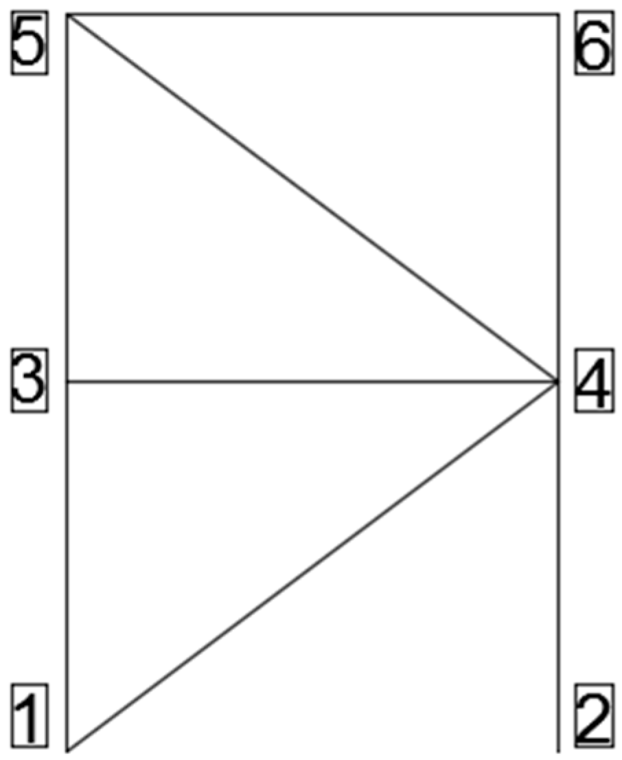
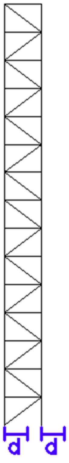
A truss is an element structure consisting of two or more bar elements, connected to each other by pins, by which each pin will support rotations around its axis only. Cranes are modeled as a truss, where this will be studied under forced vibrations and seismic loading. A freestanding crane is considered as a periodic structure where the repeated cell is shown in
Figure 3. The global nodes are numbered as in the displayed order in ANSYS.
The bar elements will differ by their cross-sectional areas, since the vertical bars hold larger loads; then, its cross-sectional area is larger than those of the horizontal and inclined bars. Hence, each element is oriented differently relative to the global coordinate system.
The element equation is expressed as:
where
,
is the angular velocity,
is the local stiffness matrix,
is the local damping matrix,
is the local mass matrix,
is the local displacement vector and
is the local loading vector.
The truss element will have two degrees of freedom (DOF) at each node: translations in the nodal x and y directions.
The bar element under study is a steel bar with characteristics represented in
Table 1.
Referenced to real-life applications, freestanding tower cranes with fixed foundations and no undercarriage supports are modeled as cranes with the repeated cell mentioned before, and they are only repeated 16 times with a total length of , including the foundation height. All dimensions are assumed relative to actual values.
Both types of loadings will be applied to the same crane structure presented, with the same repeated cell and type of material employed. Hence, the structures relative to the two different loadings will have equal stiffness, mass and damping matrices. The dynamic stiffness matrix is obtained due to the discussed approach, without the need for global assembly.
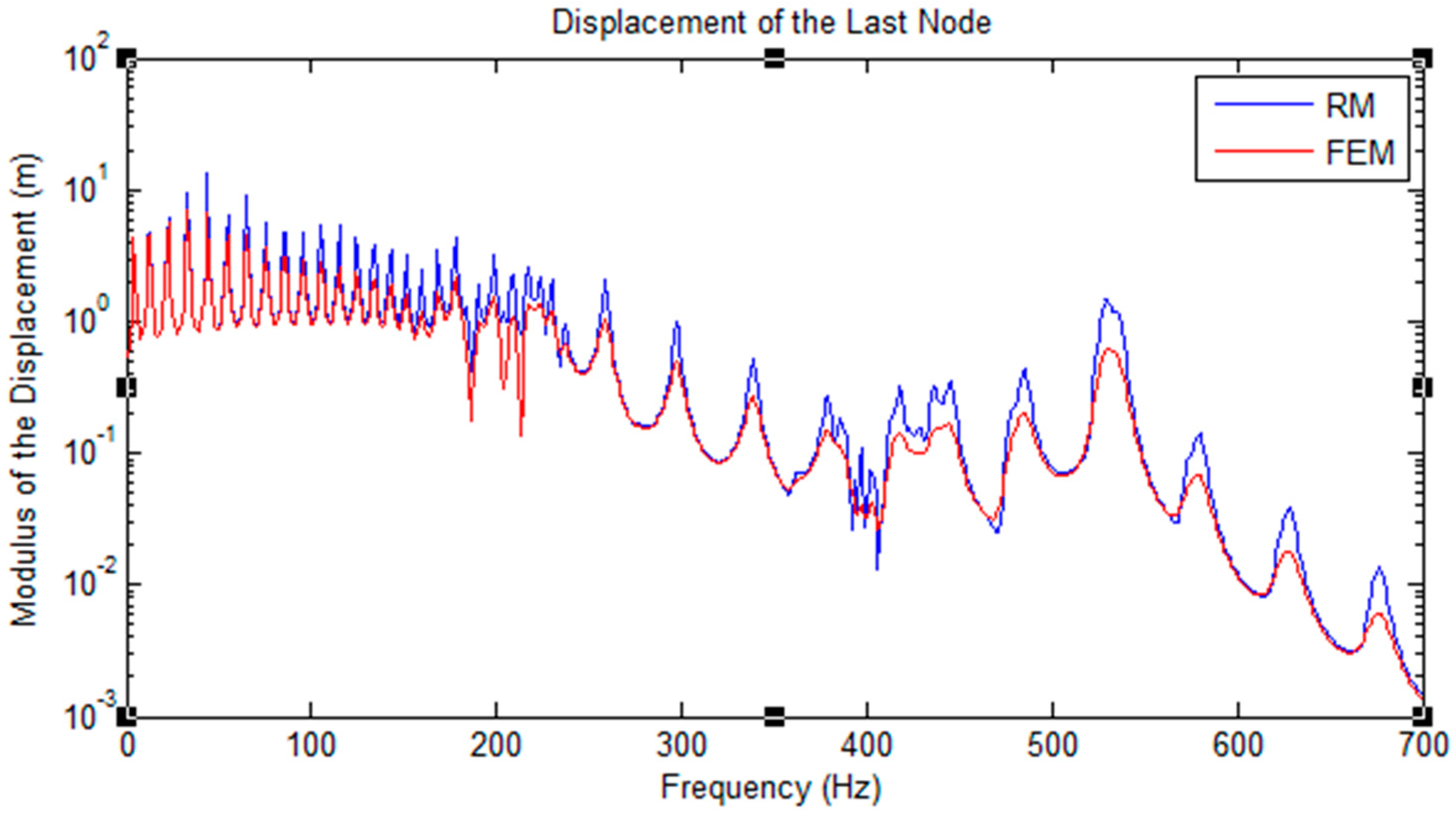
3.1.1. Truss under Forced Vibration at the Last Node
is taken for two different types of damping:
Rayleigh damping:
where
and
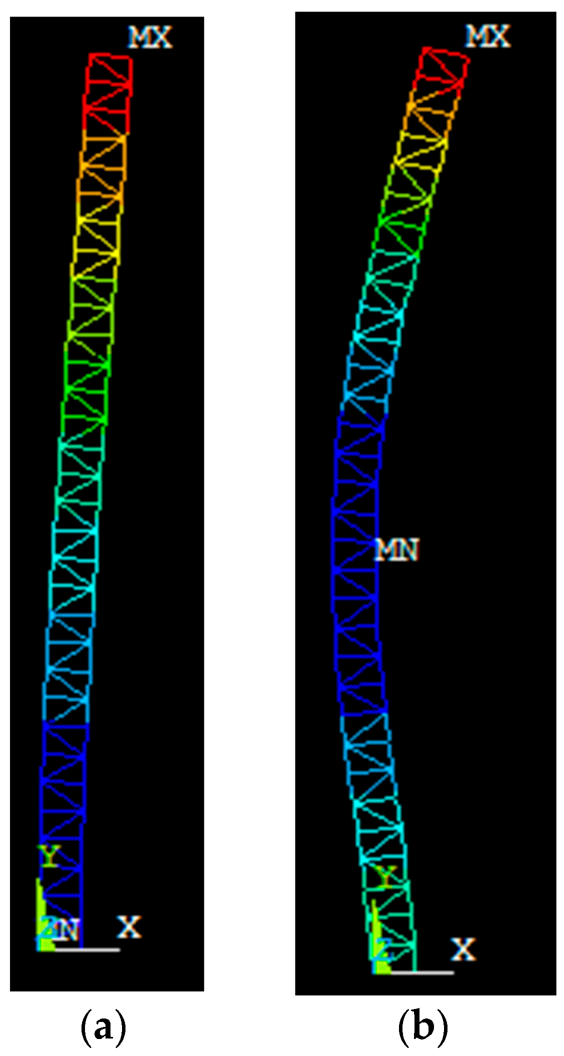
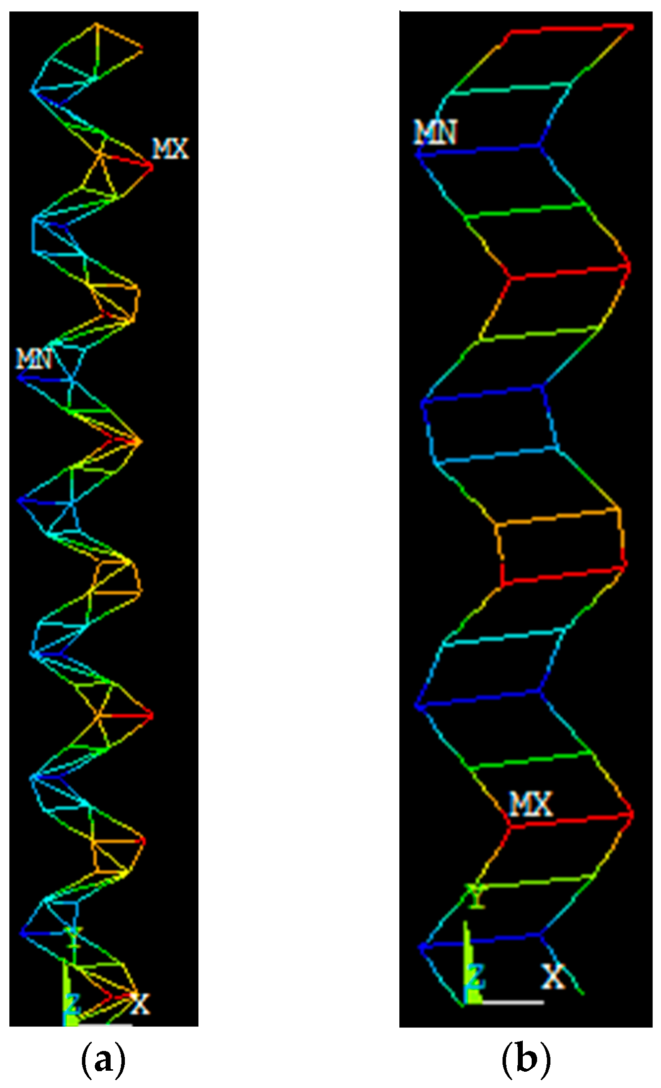
are calculated from the natural frequencies and the relative damping ratio. The natural frequencies taken are the first two natural frequencies, with their relative mode shapes shown in
Figure 4; determined by modal analysis. The damping ratio for steel material used in a footbridge damping is
[
22].
Hysteretic damping:
The dynamic stiffness matrix is demonstrated as:
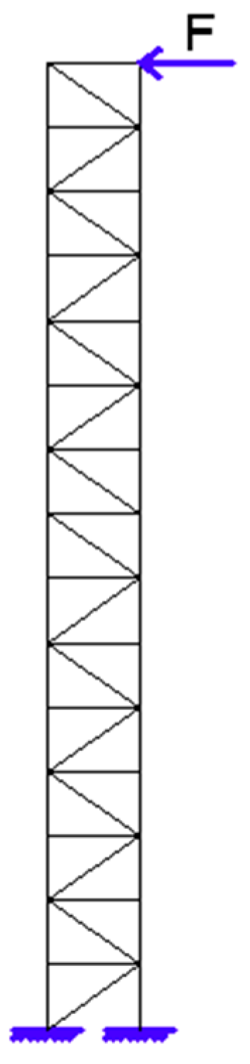
The crane interpreted is illustrated in
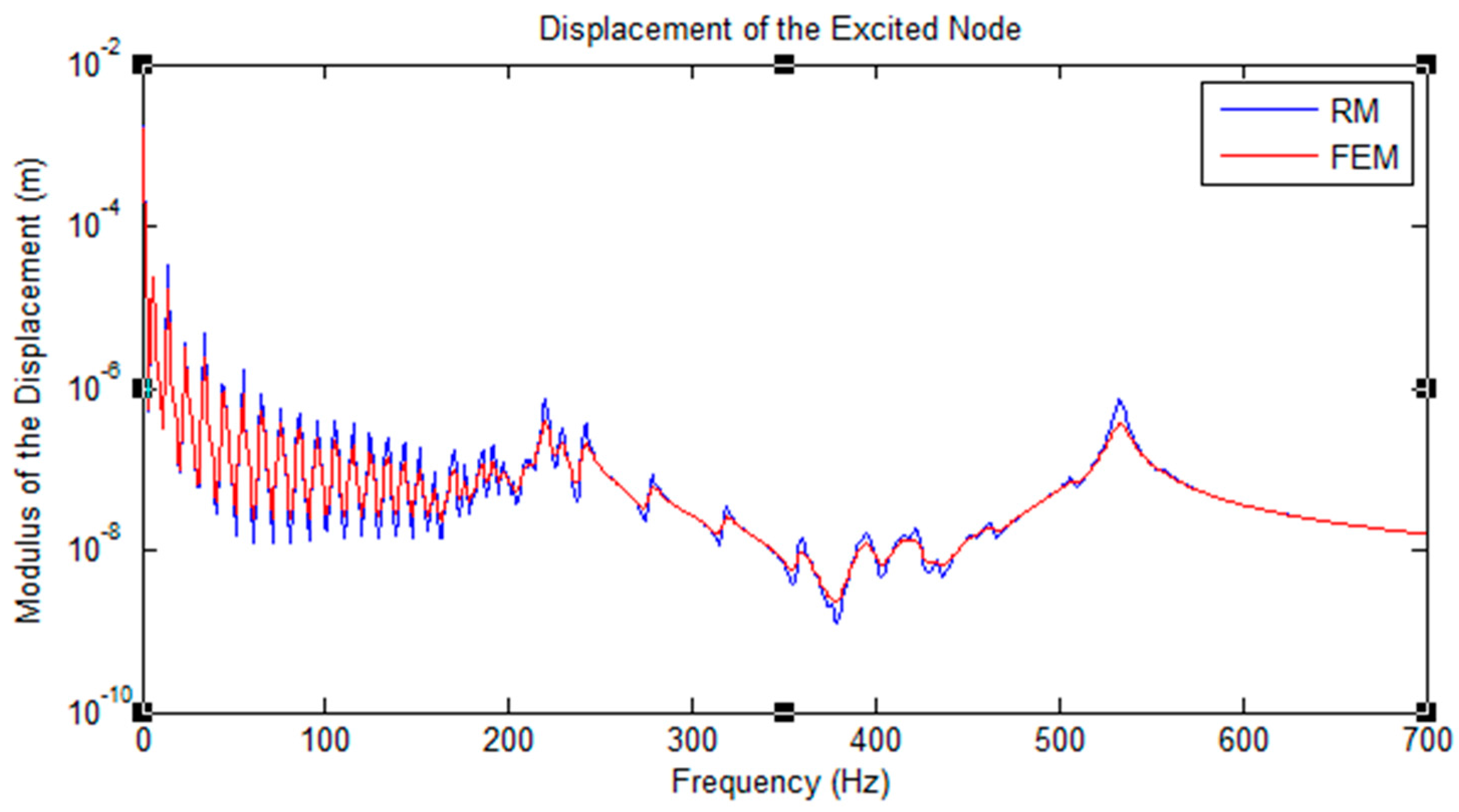
Figure 5. The last nodes of interest are under harmonic vibrations for
, where
. The fixed foundation will remove the degrees of freedom on the first two nodes in the global system, and the matrix is assembled upon a relationship between a cell and its consecutive one. The periodic structure is computed under a range of driving frequencies, for the purpose of estimating the frequency response function at the excited node.
3.1.2. Truss under Seismic Load
The truss application is applied under a second type of loading for the investigation of the frequency response function under a range of frequencies. The crane structure will be studied under hysteretic damping solely, represented by the previously shown dynamic stiffness matrix (14). The first two nodes are subjected to seismic load, which is modeled as a harmonic displacement of
, where
on the base of the structure, as shown in
Figure 6.
3.2. Frame Application under Seismic Load
Frames are structures that have a combination of beams resisting loads. Such structures are modeled to overcome large moments developed due to the applied loading. The connected node acquires three DOF, preventing displacement in the
y-direction and rotations in the
x- and
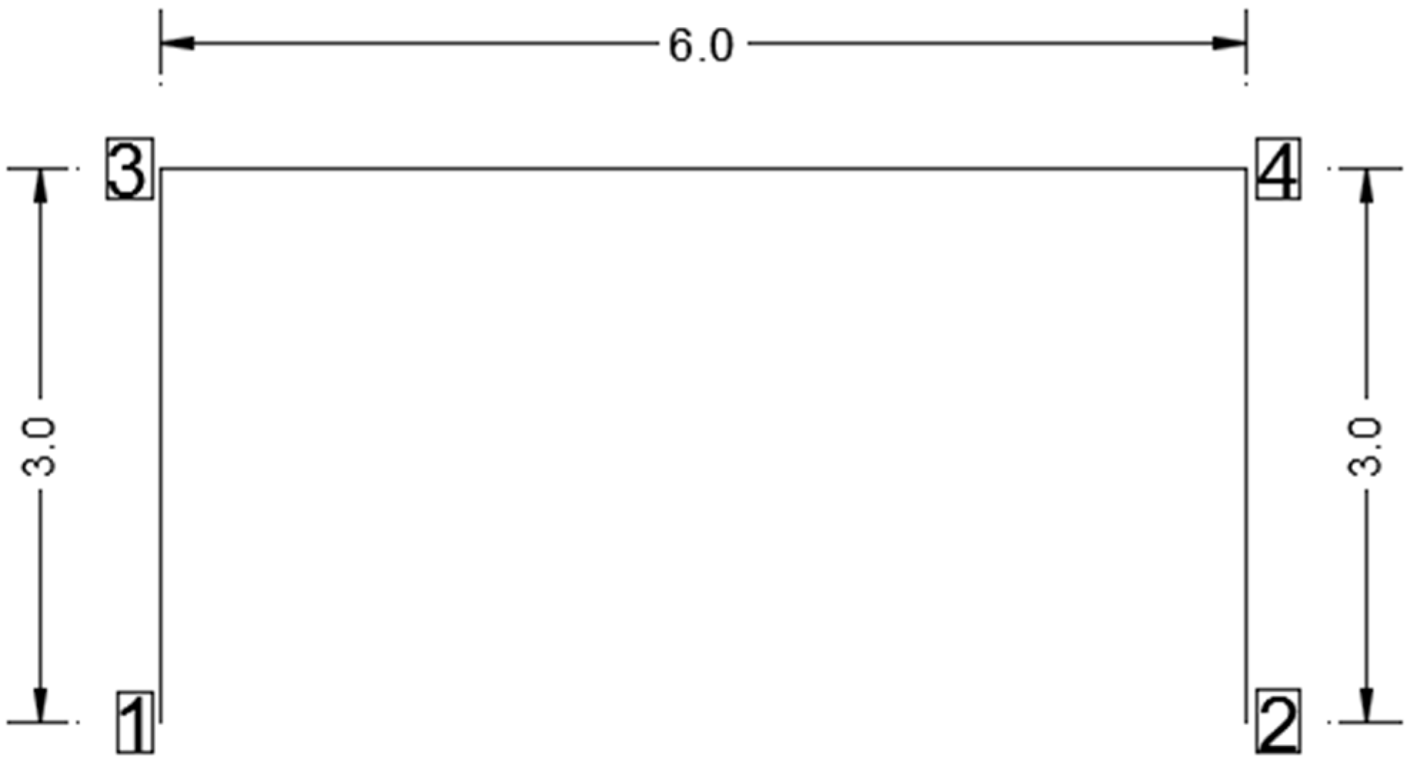
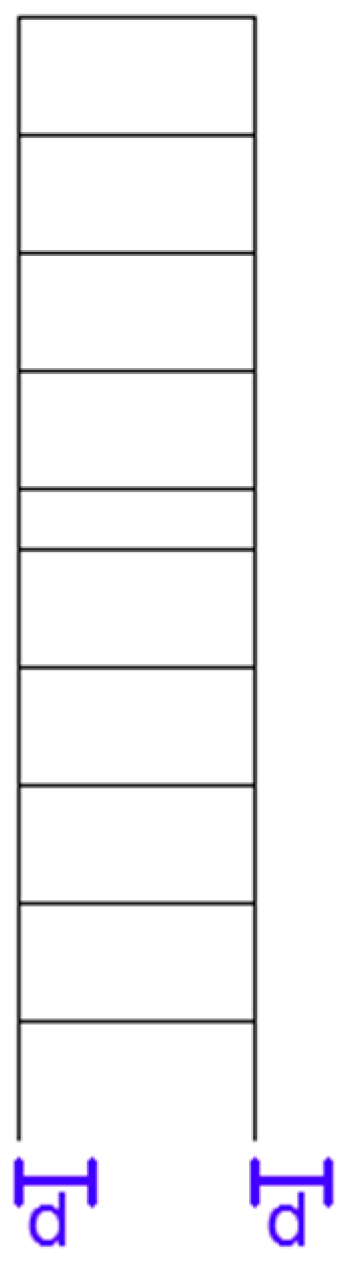
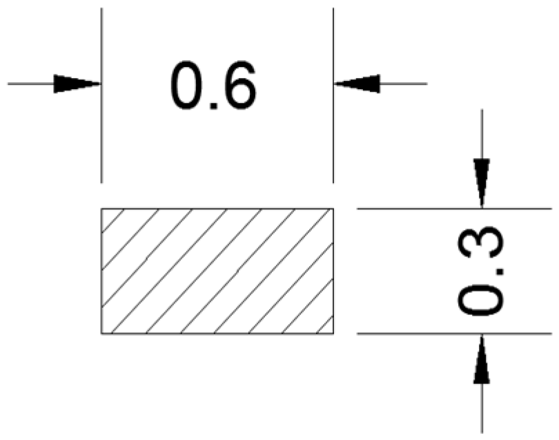
z-direction. A building under seismic load is modeled as a frame. Timoshenko beams will be studied, having four degrees of freedom. The cross-sectional dimensions of all frame elements and the repeated cell are illustrated in
Figure 7 and
Figure 8, respectively. The cell will be repeated 16 times with a total length of
.
Frame analysis for the local element is similar to the truss element. Stiffness and mass matrices (
and
) are found from the ANSYS program, and the damping matrix (
) is established using hysteretic damping, as mentioned for the truss; where the dynamic stiffness matrix is represented as:
The beam used is made up of steel with a modulus of elasticity and density similar to that of the bar element; where Young’s modulus of elasticity is
and the density is
. The nodes at the base are under a harmonic displacement of
, where
, as shown in
Figure 9. The periodic structure will be examined for a range of frequencies for computing the frequency response function.
5. Conclusions
In this paper, a further study was done on structures that cannot be designed as waveguides. Cranes and buildings were modeled as trusses and frames, respectively, under various loading. Trusses and frames have in their structural composition the inability to guide waves along their longitudinal axis. Waveguides are used in various types of applications and have different methods for accurate computations. However, structures that are not considered as waveguides consume various applications, as well, but there are no different numerical methods for easier, faster and precise computations.
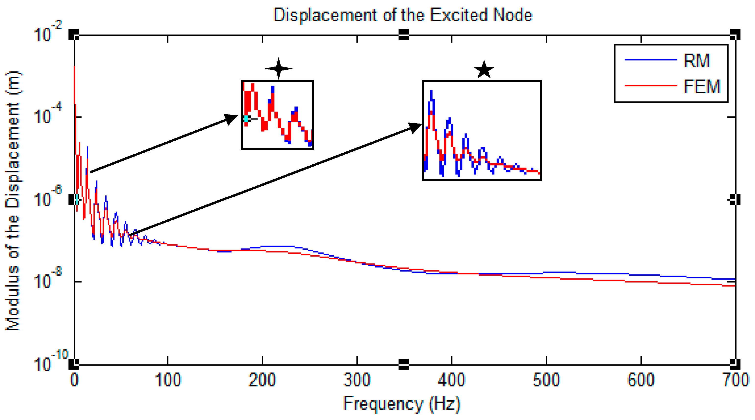
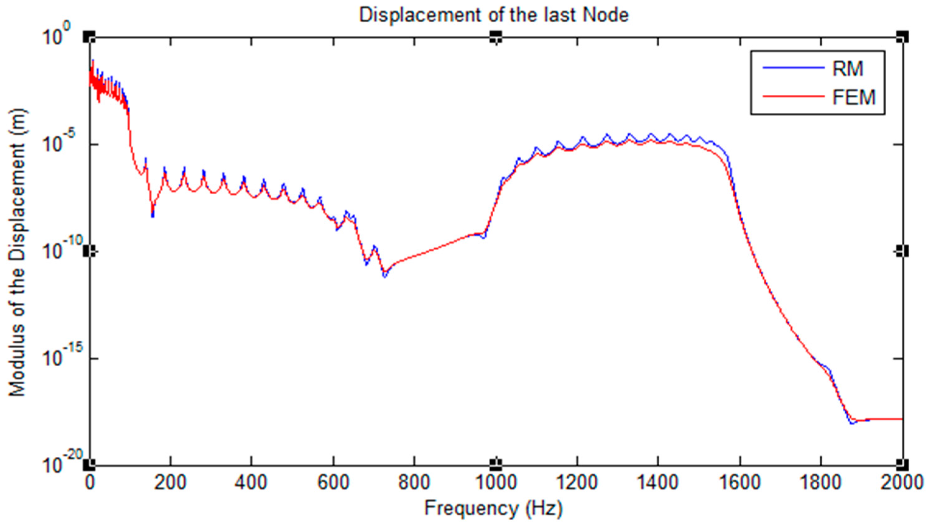
The recursive method is an approach used for calculating the frequency response function of general periodic structures. In spite of the element’s complexity, a recursive method can be employed on all types of periodic structures, as long as the internal nodes are under no load. For finding a satisfying result, a high number of cells must be considered, which will lead to a large number of computations. This method provides a solution close to that obtained from the reference method (FEM), and it decreases the time consumption. The time consumed for a steel material was observed to a have a range of ratios between 1:18 and 1:31, depending on the type of cells and the load exerted. Displacement values were nearer to that of the finite element method at low and very high frequencies. The percentage difference for the structures studied under various types of loading does not exceed 19%. Nevertheless, different materials were studied to have further support of the analysis. The plastic material had much lower time ratios, in the range between 1:22 and 1:151, while the relative percentage difference did not exceed 17%. This difference is due to the inverse of the dynamic stiffness matrix, which will lead to a slight numerical difference between the finite element method and the recursive method. Upon varying the number of forces, the time ratio lied in the range of 1:106 till 1:172, with a low percentage difference.
Future examinations include studying the effectiveness of this approach for periodic structures under a large number of forces. Expectations are that when the forces are engaged with every node, the method will not be feasible for calculating the frequency response function, since the advantage of removing the internal nodes recursively will be obsolete. Further studies include the types of cells to be repeated and the effect on the frequency response function. Moreover, a more applicable solution may be calculated by changing the type of element from linear to quadratic; therefore, vibrations at internal nodes can be computed. Otherwise, an element with a greater mesh size should be examined, since the increase in the mesh size will display the response for the internal nodes. The effect of the frequency on the modulus of displacement will be also inspected, and more complex periodic structures will be interpreted. Unsteady states in heat transfer problems may be evaluated for complex fin geometries.


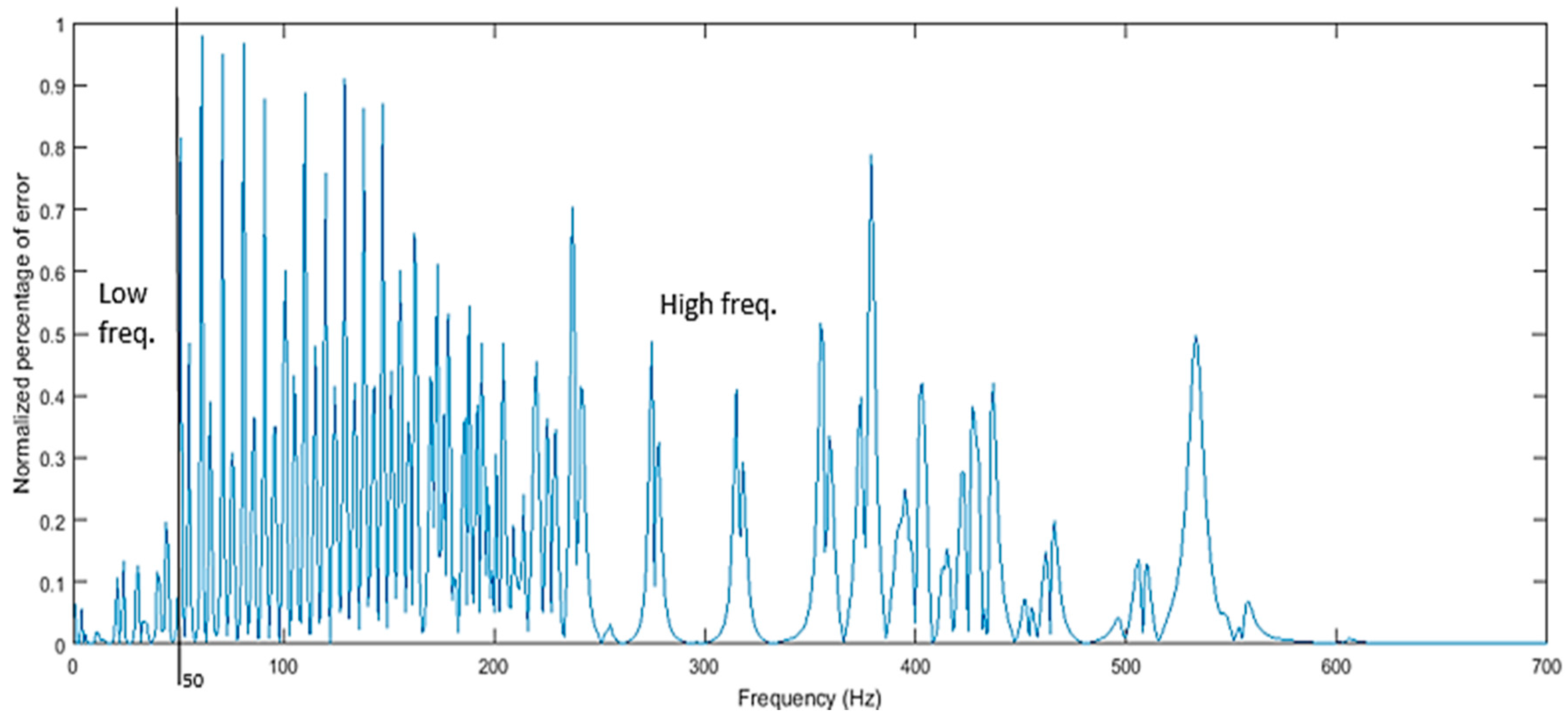
 : low frequencies;
  : high frequencies. RM, recursive method.


