Psychometric Modeling to Identify Examinees’ Strategy Differences during Testing


Abstract
1. Introduction
1.1. Between-Person Differences in Strategies
1.2. Within-Person Changes in Strategies
- (1)
- Can the transition patterns be directly modeled and hence used to inform future test administration practice?
- (2)
- Can information from these transition patterns be used to adjust the ability estimates in an effort to improve the underlying validity of the measure?
2. Study 1: Mixture Models to Identify Strategy Differences
2.1. Background: Mixture Models
2.2. Method
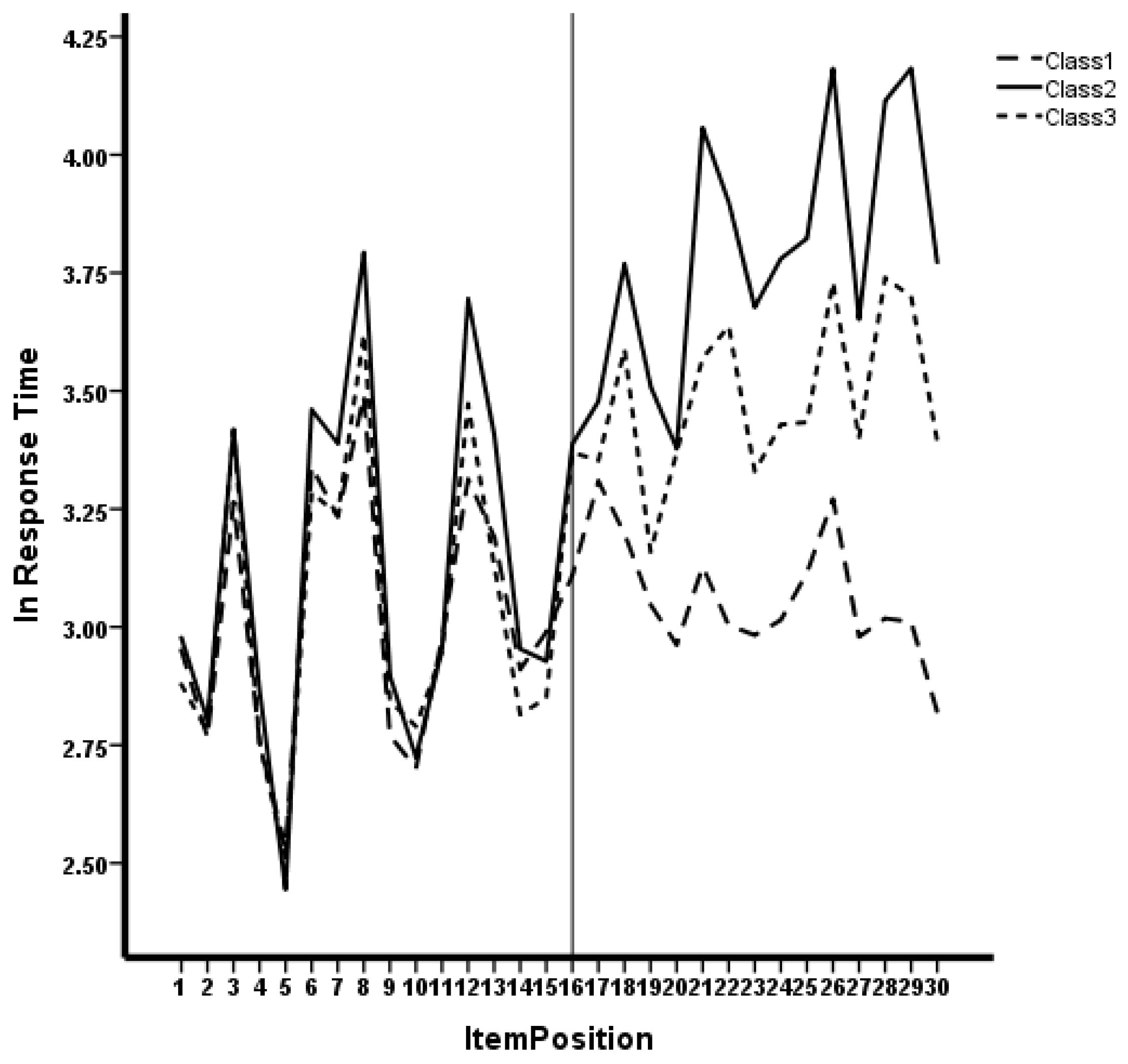
2.3. Results
2.4. Discussion
3. Study 2: Intra-Individual Variability in Response Process
3.1. Background
3.2. Method
3.3. Alternative Trims
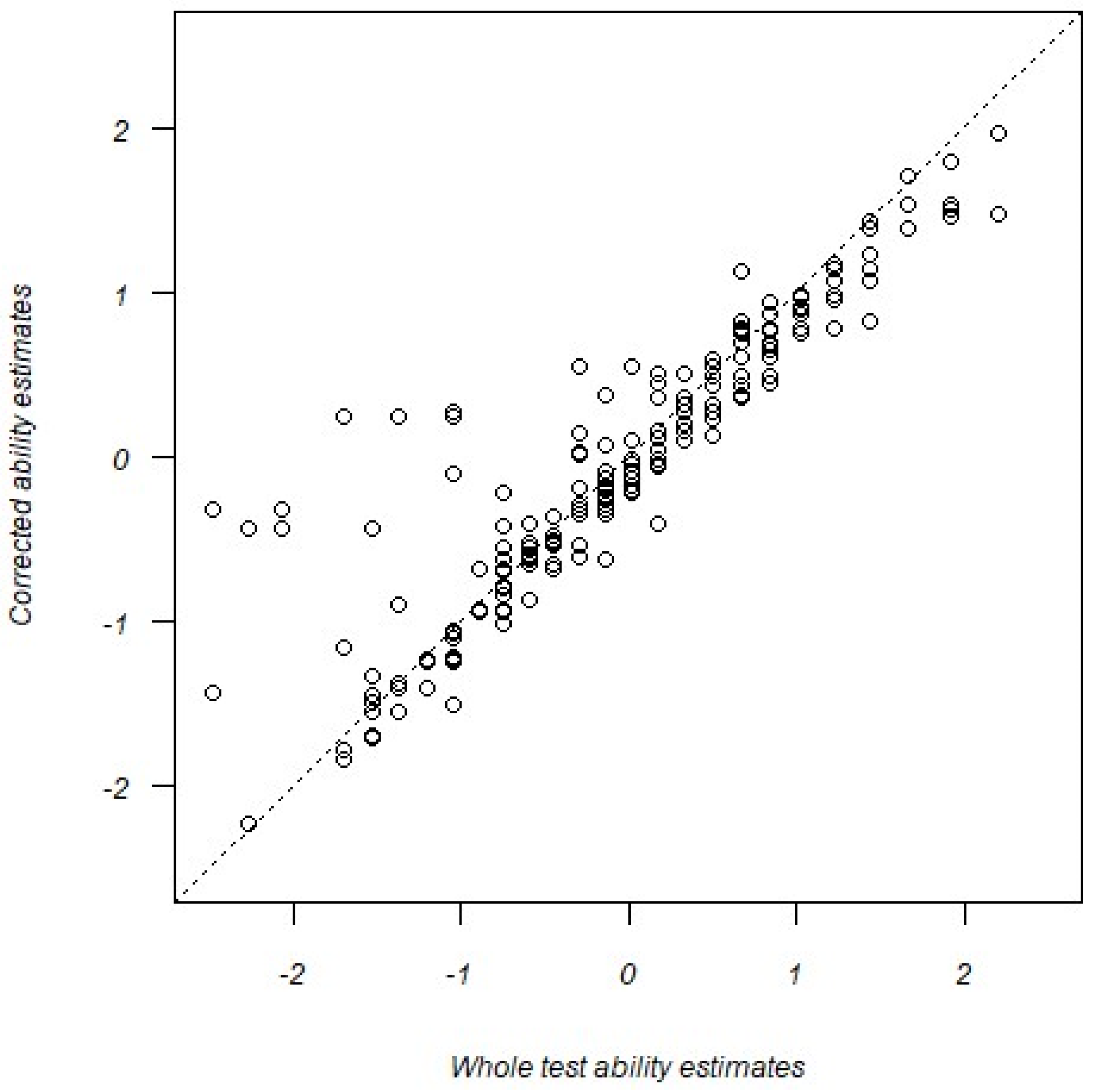
3.4. Results
3.5. Discussion
4. Discussion and Summary
Author Contributions
Funding
Institutional Review Board Statement
Informed Consent Statement
Data Availability Statement
Acknowledgments
Conflicts of Interest
Appendix A. Reliability Adjusted Validity Coefficient
Appendix A.1. Calculation
Appendix A.2. Testing for Significance
References
- Albano, Anthony D. 2013. Multilevel modeling of item position effects. Journal of Educational Measurement 50: 408–26. [Google Scholar] [CrossRef]
- Bethell-Fox, Charles E., and Roger N. Shepard. 1988. Mental rotation: Effects of stimulus complexity and familiarity. Journal of Experimental Psychology: Human Perception and Performance 14: 12. [Google Scholar] [CrossRef]
- Bolt, Daniel M., Allan S. Cohen, and James A. Wollack. 2002. Item parameter estimation under conditions of test speededness: Application of a mixture Rasch model with ordinal constraints. Journal of Educational Measurement 4: 331–48. [Google Scholar] [CrossRef]
- Busemeyer, Jerome R., and Adele Diederich. 2010. Cognitive Modeling. Thousand Oaks: Sage. [Google Scholar]
- Davis, Jeff, and Abdullah Ferdous. 2005. Using item difficulty and item position to measure test fatigue. Paper presented at the Annual Meeting of the American Educational Research Association, Montreal, QC, Canada, April 11–15. [Google Scholar]
- Eignor, Daniel R. 2014. Standards for Educational and Psychological Testing. Washington, DC: AERA, APA and NCME. [Google Scholar]
- Embretson, Susan E. 2007. Mixed Rasch model for measurement in cognitive psychology. In Multivariate and Mixture Distribution Rasch Models: Extensions and Applications. Edited by Matthias von Davier and Claus H. Carstensen. Amsterdam: Springer, pp. 235–54. [Google Scholar]
- Embretson, Susan E. 2023. Understanding examinees’ item responses through cognitive modeling of response accuracy and response times. Large-Scale Assessments in Education 11: 9. [Google Scholar] [CrossRef]
- Frick, Hannah, Carolin Strobl, Friedrich Leisch, and Achim Zeileis. 2012. Flexible Rasch Mixture Models with Package Psychomix. Journal of Statistical Software 48: 1–25. Available online: http://www.jstatsoft.org/v48/i07/ (accessed on 6 June 2023). [CrossRef]
- Frick, Hannah. 2022. Package ‘Psychomix’. Available online: https://cran.r-project.org/web/packages/psychomix/psychomix.pdf (accessed on 12 June 2023).
- Gluck, Judith, and Sylvia Fitting. 2003. Spatial strategy selection: Interesting incremental information. International Journal of Testing 3: 293–308. [Google Scholar] [CrossRef]
- Goegebeur, Yuri, Paul De Boeck, James A. Wollack, and Allan S. Cohen. 2008. A speeded item response model with gradual process change. Psychometrika 73: 65–87. [Google Scholar] [CrossRef]
- Goldhammer, Frank. 2015. Measuring ability, speed, or both? Challenges, psychometric solutions, and what can be gained from experimental control. Measurement: Interdisciplinary Research and Perspectives 13: 133–64. [Google Scholar] [CrossRef] [PubMed]
- Kingston, Neal M., and Neil J. Dorans. 1982. The effect of the position of an item within a test on item responding behavior: An analysis based on item response theory. ETS Research Report Series 1982: i-26. [Google Scholar] [CrossRef]
- Mislevy, Robert J., and Norman Verhelst. 1990. Modeling item responses when different subjects employ different solution strategies. Psychometrika 55: 195–215. [Google Scholar] [CrossRef]
- Molenaar, Dylan, and Paul DeBoeck. 2018. Response mixture modeling: Accounting for heterogeneity in item characteristics across response times. Psychometrika 83: 279–97. [Google Scholar] [CrossRef] [PubMed]
- Molenaar, Dylan, Daniel Oberski, Jeroen Vermunt, and Paul De Boeck. 2016. Hidden Markov item response theory models for responses and response times. Multivariate Behavioral Research 51: 606–26. [Google Scholar] [CrossRef] [PubMed]
- Qian, Hong, Dorota Staniewska, Mark Reckase, and Ada Woo. 2016. Using response time to detect item preknowledge in computer-based licensure examinations. Educational Measurement: Issues and Practice 35: 38–47. [Google Scholar] [CrossRef]
- Rost, Jürgen, and Matthias von Davier. 1995. Mixture Distribution Rasch Models. In Rasch Models: Foundation, Recent Developments and Applications. Edited by Gerhard Fischer and Ivo Molenaar. New York: Springer, pp. 257–68. [Google Scholar]
- Schultz, Katherine. 1991. The contribution of solution strategy to spatial performance. Canadian Journal of Psychology/Revue Canadienne de Psychologie 45: 474. [Google Scholar] [CrossRef]
- Smallwood, Jonathan, John B Davies, Derek Heim, Frances Finnigan, Megan Sudberry, Rory O’Connor, and Marc Obonsawin. 2004. Subjective experience and the attentional lapse: Task engagement and disengagement during sustained attention. Consciousness and Cognition 13: 657–90. [Google Scholar] [CrossRef] [PubMed]
- Smallwood, Jonathan, Marc Obonsawin, and Derek Heim. 2003. Task unrelated thought: The role of distributed processing. Consciousness and Cognition 12: 169–89. [Google Scholar] [CrossRef] [PubMed]
- Unsworth, Nash, Matthew K. Robison, and Ashley L. Miller. 2021. Individual differences in lapses of attention: A latent variable analysis. Journal of Experimental Psychology: General 150: 1303. [Google Scholar] [CrossRef]
- van der Linden, Wim J. 2006. A lognormal model for response times on test items. Journal of Educational and Behavioral Statistics 31: 181–204. [Google Scholar] [CrossRef]
- van der Linden, Wim J., and Fanmin Guo. 2008. Bayesian procedures for identifying aberrant response-time patterns in adaptive testing. Psychometrika 73: 365–84. [Google Scholar] [CrossRef]
- von Davier, Matthias. 2001. WINMIRA 2001 Software Manual. IPN: Institute for Science Education. Available online: http://208.76.80.46/~svfklumu/wmira/winmiramanual.pdf (accessed on 5 May 2023).
- von Davier, Matthias. 2005. mdltm: Software for the General Diagnostic Model and for Estimating Mixtures of Multidimensional Discrete Latent Traits Models [Computer Software]. Princeton: ETS. [Google Scholar]
- von Davier, Matthias. 2009. The mixture general diagnostic model. In Advances in Latent Variable Mixture Models. Edited by Gregory R. Hancock and Karen M. Samuelson. Charlotte: Information Age Publishing, pp. 255–74. [Google Scholar]
- Wise, Steven L., and Christine E. DeMars. 2006. An application of item response time: The effort-moderated IRT model. Journal of Educational Measurement 43: 19–38. [Google Scholar] [CrossRef]
- Yamamoto, Kentaro. 1989. HYBRID model of IRT and latent class models. In ETS Research Report RR89-41. Princeton: Educational Testing Service. [Google Scholar]
- Yamamoto, Kentaro, and Howard Everson. 1997. Modeling the effects of test length and test time on parameter estimation using the HYBRID model. In Applications of Latent Trait and Latent Class Models in the Social Sciences. Edited by Jürgen Rost and Rolf Langeheine. Munster: Waxmann, pp. 89–98. [Google Scholar]
- Zhu, Hongyue, Hong Jiao, Wei Gao, and Xiangbin Meng. 2023. Bayesian Change-Point Analysis Approach to Detecting Aberrant Test-Taking Behavior Using Response Times. Journal of Educational and Behavioral Statistics 48: 490–520. [Google Scholar] [CrossRef]
- Zopluglu, Cengiz. 2020. A finite mixture item response theory model for continuous measurement outcomes. Educational and Psychological Measurement 80: 346–64. [Google Scholar] [CrossRef] [PubMed]


| Classes | Class Sizes | -2lnL | Number Parameters | AIC | Χ2 |
|---|---|---|---|---|---|
| One class | 1.00 | 9664.96 | 31 | 9727.69 | --- |
| Two class | .61, .39 | 9564.86 | 63 | 9690.85 | 100.10 ** |
| Three class | .46, .31, .23 | 9506.48 | 95 | 9696.49 | 58.38 * |
| Class Variable | Mean | SD | Correlations MnlnRT AFQT | ||
|---|---|---|---|---|---|
| 1 N = 135 | Trait | −.235 | .889 | .656 ** | .231 * |
| Mn lnRT | 3.038 | .611 | 1.000 | .143 | |
| AFQT | 214.510 | 15.440 | .143 | 1.000 | |
| 2 N = 98 | Trait | 1.689 | .819 | .109 | .511 ** |
| Mn lnRT | 3.446 | .289 | 1.000 | .119 | |
| AFQT | 230.121 | 15.485 | .119 | 1.000 | |
| 3 N = 68 | Trait | .746 | .866 | .515 ** | .509 ** |
| Mn lnRT | 3.251 | .362 | 1.000 | .239 | |
| AFQT | 223.064 | 16.880 | .239 | 1.000 | |
| Regression: Cognitive Modeling | ||||||||
|---|---|---|---|---|---|---|---|---|
| Variable Class | Mean | SD | rlnRT | R | Memory Load β1 | Unique Elements β2 | Position Added R | |
| Item Difficulty | 1 | .000 | 1.201 | .444 * | .613 ** | .469 ** | .302 + | .717 ** |
| 2 | .000 | 1.890 | .754 ** | .607 ** | .534 ** | .190 | .645 ** | |
| 3 | .000 | 1.548 | .642 ** | .613 ** | .512 ** | .240 | .629 ** | |
| Response Time | 1 | 3.038 | .215 | 1.000 | .128 | .038 | .114 | .130 |
| 2 | 3.445 | .470 | 1.000 | .659 ** | .607 ** | .153 | .765 ** | |
| 3 | 3.250 | .342 | 1.000 | .631 ** | .583 ** | .142 | .697 * | |
| Initial State Distribution | Stationary Distribution | |
|---|---|---|
| State 1: Construct-driven | .948 | .700 |
| State 2: Erratic response | .052 | .300 |
| Construct-driven | 0.187 | .67 |
| Erratic | 1.647 | .26 |
| r | % Variance | ||
|---|---|---|---|
| Original Data (No Trim) | .559 | .312 | |
| Change-point Model (residual analysis) | .628 * | .394 | |
| Change-point Model (response speed shift) | .566 * | .320 | |
| Markov Process Model | .591 * | .349 | |
| Data with removal for: | |||
| All negative residuals | .565 * | .319 | |
| <−0.5 SD residuals | .550 * | .303 | |
| <−1.0 SD residuals | .569 * | .324 | |
| <−1.5 SD residuals | .565 * | .319 | |
| <−2.0 SD residuals | .568 * | .317 | |
| <−2.5 SD residuals | .563 * | .319 | |
| <−3.0 SD residuals | .563 | .317 | |
| <−3.5 SD residuals | .562 | .316 | |
| <−5.0 SD residuals | .559 | .312 | |
| <−6.0 SD residuals | .559 | .312 | |
Disclaimer/Publisher’s Note: The statements, opinions and data contained in all publications are solely those of the individual author(s) and contributor(s) and not of MDPI and/or the editor(s). MDPI and/or the editor(s) disclaim responsibility for any injury to people or property resulting from any ideas, methods, instructions or products referred to in the content. |
© 2024 by the authors. Licensee MDPI, Basel, Switzerland. This article is an open access article distributed under the terms and conditions of the Creative Commons Attribution (CC BY) license (https://creativecommons.org/licenses/by/4.0/).
Share and Cite
Hauenstein, C.E.; Embretson, S.E.; Kim, E. Psychometric Modeling to Identify Examinees’ Strategy Differences during Testing. J. Intell. 2024, 12, 40. https://doi.org/10.3390/jintelligence12040040
Hauenstein CE, Embretson SE, Kim E. Psychometric Modeling to Identify Examinees’ Strategy Differences during Testing. Journal of Intelligence. 2024; 12(4):40. https://doi.org/10.3390/jintelligence12040040
Chicago/Turabian StyleHauenstein, Clifford E., Susan E. Embretson, and Eunbee Kim. 2024. "Psychometric Modeling to Identify Examinees’ Strategy Differences during Testing" Journal of Intelligence 12, no. 4: 40. https://doi.org/10.3390/jintelligence12040040
APA StyleHauenstein, C. E., Embretson, S. E., & Kim, E. (2024). Psychometric Modeling to Identify Examinees’ Strategy Differences during Testing. Journal of Intelligence, 12(4), 40. https://doi.org/10.3390/jintelligence12040040