An Investigation of Growth Mixture Models for Studying the Flynn Effect

Abstract
:1. Introduction
1.1. Mixture Models
1.2. Current Study
2. Method
2.1. Monte Carlo Study
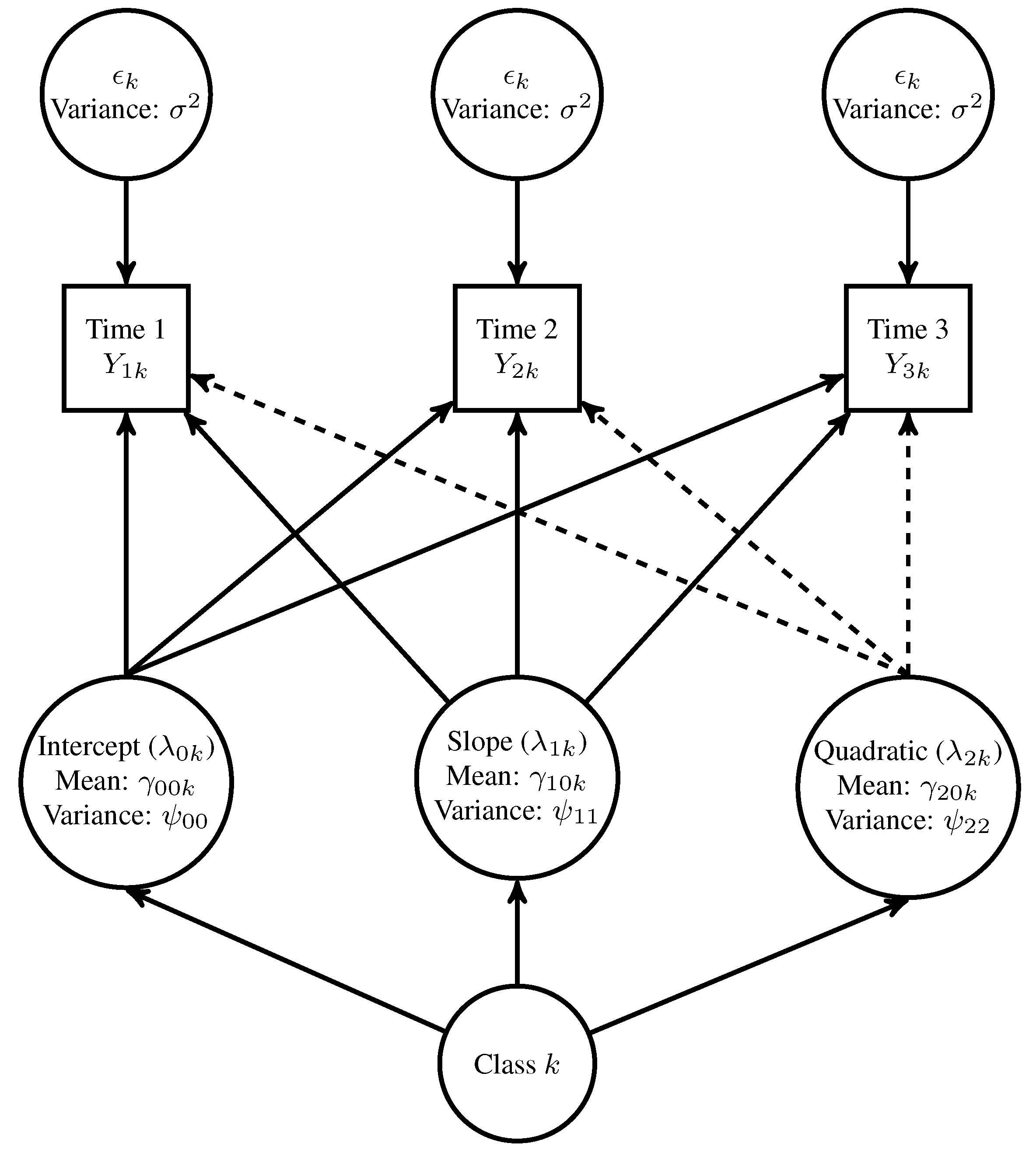
2.1.1. Population Models


2.1.2. Design Factors

| Factor | Level 1 | Level 2 |
|---|---|---|
| Class Prevalence (Class 1/Class 2) | 0.40/0.60 | 0.30/0.70 |
| Sample Size | 200 | 800 |
| Measure Reliability | 0.80 | 0.95 |
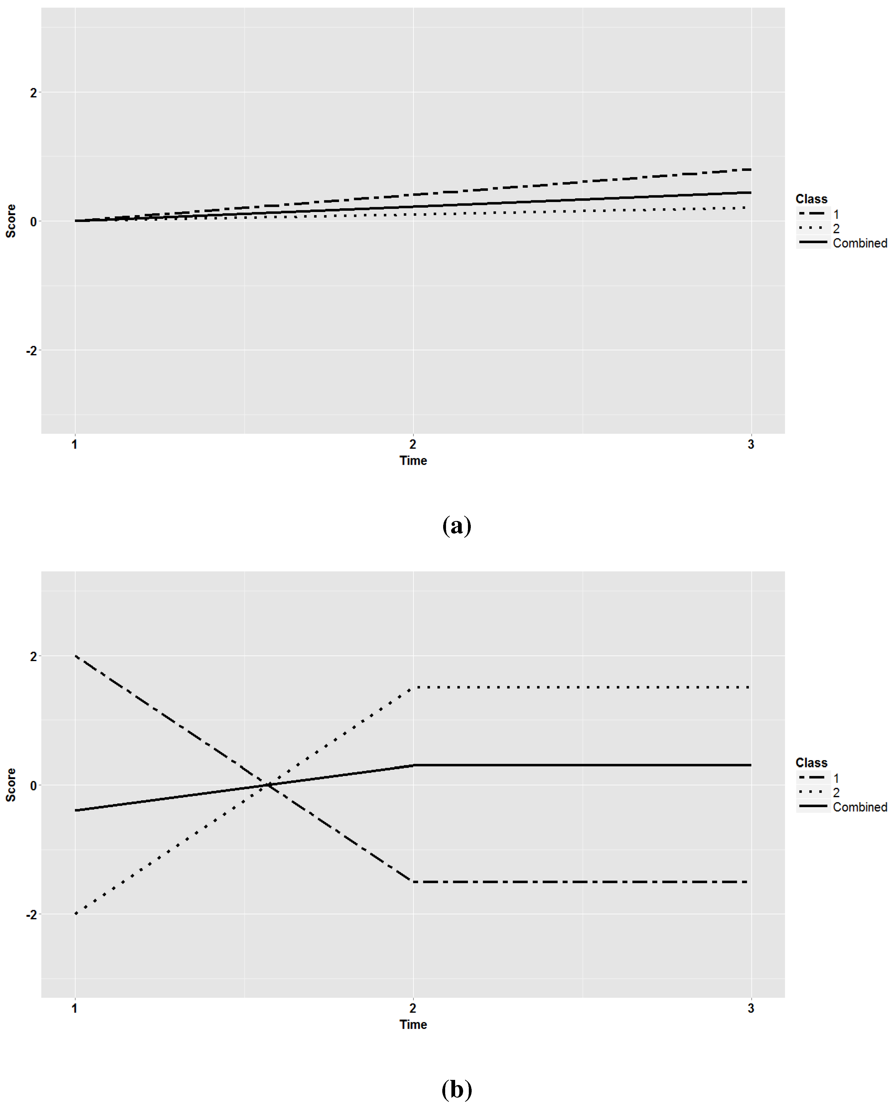
| Growth Pattern | Linear (Not Crossed) | Quadratic (Crossed) |
| Growth Pattern | ||||
|---|---|---|---|---|
| Class Prevalence | Reliability | Sample Size | Crossing | Non-Crossing |
| = 0.40, = 0.60 | 0.80 | 200 | 0.20 | 0.63 |
| = 0.40, = 0.60 | 0.80 | 800 | 0.20 | 0.63 |
| = 0.40, = 0.60 | 0.95 | 200 | 0.20 | 1.07 |
| = 0.40, = 0.60 | 0.95 | 800 | 0.20 | 1.07 |
| = 0.30, = 0.70 | 0.80 | 200 | 0.43 | 0.55 |
| = 0.30, = 0.70 | 0.80 | 800 | 0.43 | 0.55 |
| = 0.30, = 0.70 | 0.95 | 200 | 0.43 | 0.95 |
| = 0.30, = 0.70 | 0.95 | 800 | 0.43 | 0.95 |
2.2. Data Generation
2.3. Fit Indices to Aid in the Growth Mixture Model Selection
2.3.1. Absolute Model Fit
2.3.2. Lo–Mendell–Rubin Likelihood Ratio Test
2.3.3. Relative Fit Indices
| Index | Abbreviation | Formula |
|---|---|---|
| Akaike information criteria | AIC | |
| Consistent AIC | CAIC | |
| Corrected AIC | AICc | AIC |
| Bayesian information criteria | BIC | |
| Sample size adjusted BIC | SSBIC | |
| Draper’s information criterion | DIC |
2.3.4. Classification Certainty
2.4. Analysis
2.5. Software
3. Results
3.1. Monte Carlo Study
| Accuracy | |
|---|---|
| Fit Index | (% Correct) |
| Akaike information criterion (AIC) | 57.1 |
| Corrected Akaike information criterion (AICc) | 66.7 |
| Consistent Akaike information criterion (CAIC) | 99.9 |
| Bayesian information criterion (BIC) | 99.8 |
| Sample size adjusted BIC (SSBIC) | 79.0 |
| Draper’s information criterion (DIC) | 96.8 |
| Integrated classification likelihood with BIC approximation (ICL-BIC) | 89.5 |
| Lo–Mendell–Rubin likelihood ratio test (LMR) | 54.4 |
| Fit Index | ||||||||||
|---|---|---|---|---|---|---|---|---|---|---|
| Class Prevalence | Reliability | Sample Size | AIC | AICc | CAIC | BIC | SSBIC | DIC | ICL-BIC | LMR |
| Crossing Growth Pattern | ||||||||||
| π1 = 0.40, π2 = 0.60 | 0.80 | 200 | 60 | 75 | 100 | 100 | 66 | 96 | 100 | 76 |
| π1 = 0.40, π2 = 0.60 | 0.80 | 800 | 58 | 63 | 100 | 100 | 96 | 100 | 100 | 73 |
| π1 = 0.40, π2 = 0.60 | 0.95 | 200 | 60 | 76 | 100 | 100 | 67 | 96 | 100 | 78 |
| π1 = 0.40, π2 = 0.60 | 0.95 | 800 | 60 | 64 | 100 | 100 | 96 | 100 | 100 | 73 |
| π1 = 0.30, π2 = 0.70 | 0.80 | 200 | 58 | 74 | 100 | 100 | 64 | 96 | 100 | 78 |
| π1 = 0.30, π2 = 0.70 | 0.80 | 800 | 58 | 62 | 100 | 100 | 97 | 100 | 100 | 74 |
| π1 = 0.30, π2 = 0.70 | 0.95 | 200 | 58 | 74 | 100 | 100 | 66 | 96 | 100 | 79 |
| π1= 0.30, π2 = 0.70 | 0.95 | 800 | 60 | 63 | 100 | 100 | 97 | 100 | 100 | 73 |
| Non-Crossing Growth Pattern | ||||||||||
| π1 = 0.40, π2 = 0.60 | 0.80 | 200 | 50 | 66 | 100 | 99 | 58 | 92 | 66 | 9 |
| π1 = 0.40, π2 = 0.60 | 0.80 | 800 | 59 | 63 | 100 | 100 | 96 | 99 | 73 | 13 |
| π1 = 0.40, π2 = 0.60 | 0.95 | 200 | 55 | 68 | 100 | 100 | 60 | 93 | 77 | 24 |
| π1 = 0.40, π2 = 0.60 | 0.95 | 800 | 62 | 65 | 100 | 100 | 96 | 99 | 94 | 80 |
| π1 = 0.30, π2 = 0.70 | 0.80 | 200 | 50 | 66 | 100 | 100 | 57 | 93 | 68 | 9 |
| π1 = 0.30, π2 = 0.70 | 0.80 | 800 | 57 | 61 | 100 | 100 | 96 | 99 | 74 | 17 |
| π1 = 0.30, π2 = 0.70 | 0.95 | 200 | 50 | 65 | 100 | 99 | 58 | 93 | 85 | 29 |
| π1 = 0.30, π2 = 0.70 | 0.95 | 800 | 60 | 64 | 100 | 100 | 94 | 99 | 97 | 84 |
3.1.1. Relative Fit Indices
3.1.2. Classification Certainty
3.1.3. Lo–Mendell–Rubin Likelihood Ratio Test
3.2. National Intelligence Tests
| Variable | Class 1 | Class 2 | Combined |
|---|---|---|---|
| Membership | |||
| n | 89 (24.7%) | 272 (75.4%) | 361 |
| Female | 43 (48.3%) | 169 (62.1%) | |
| Age | |||
| 12 Years | 12 (13.5%) | 35 (12.9%) | |
| 13 Years | 66 (74.2%) | 155 (57.0%) | |
| 14 Years | 11 (12.4%) | 82 (30.2%) | |
| NIT Scores | |||
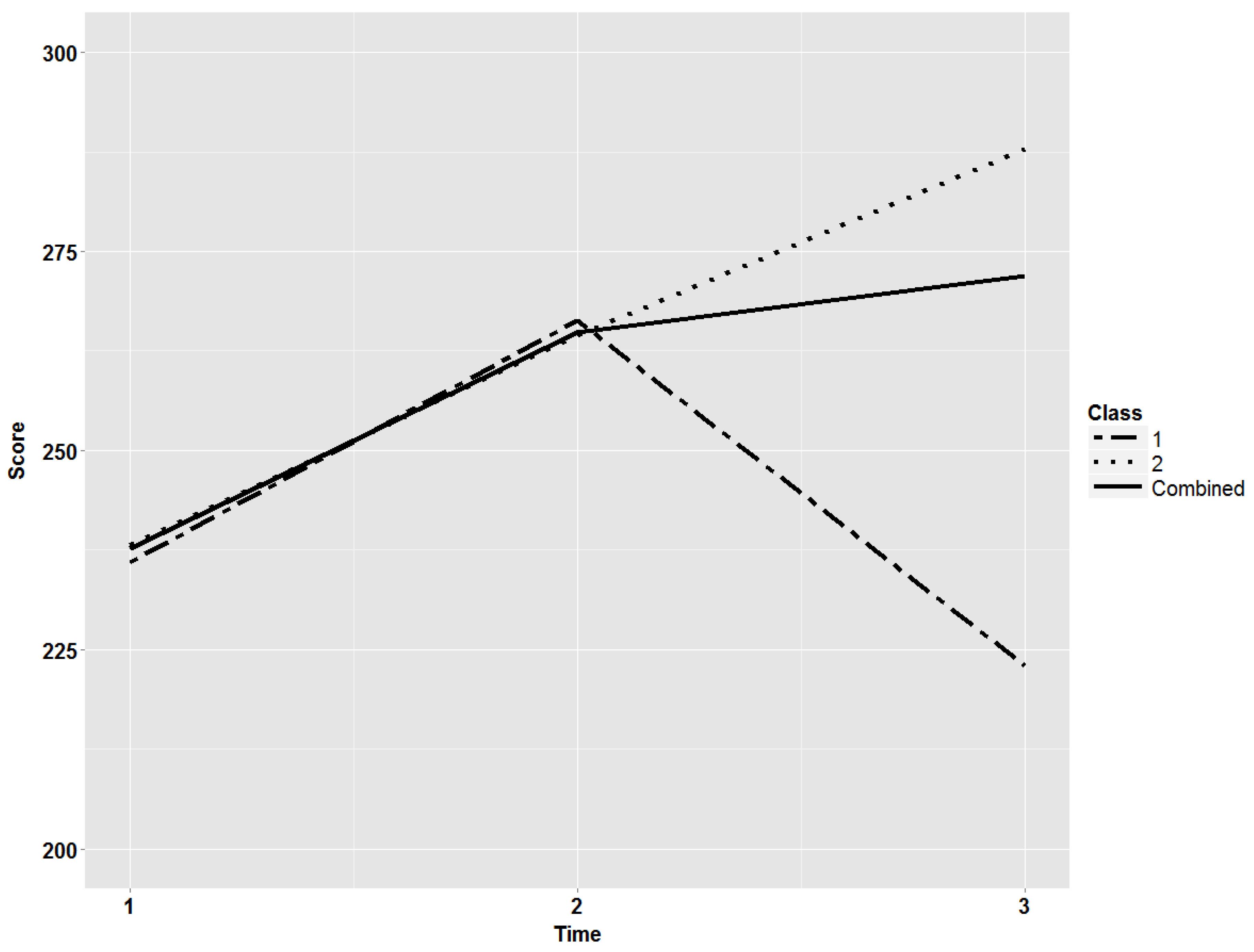
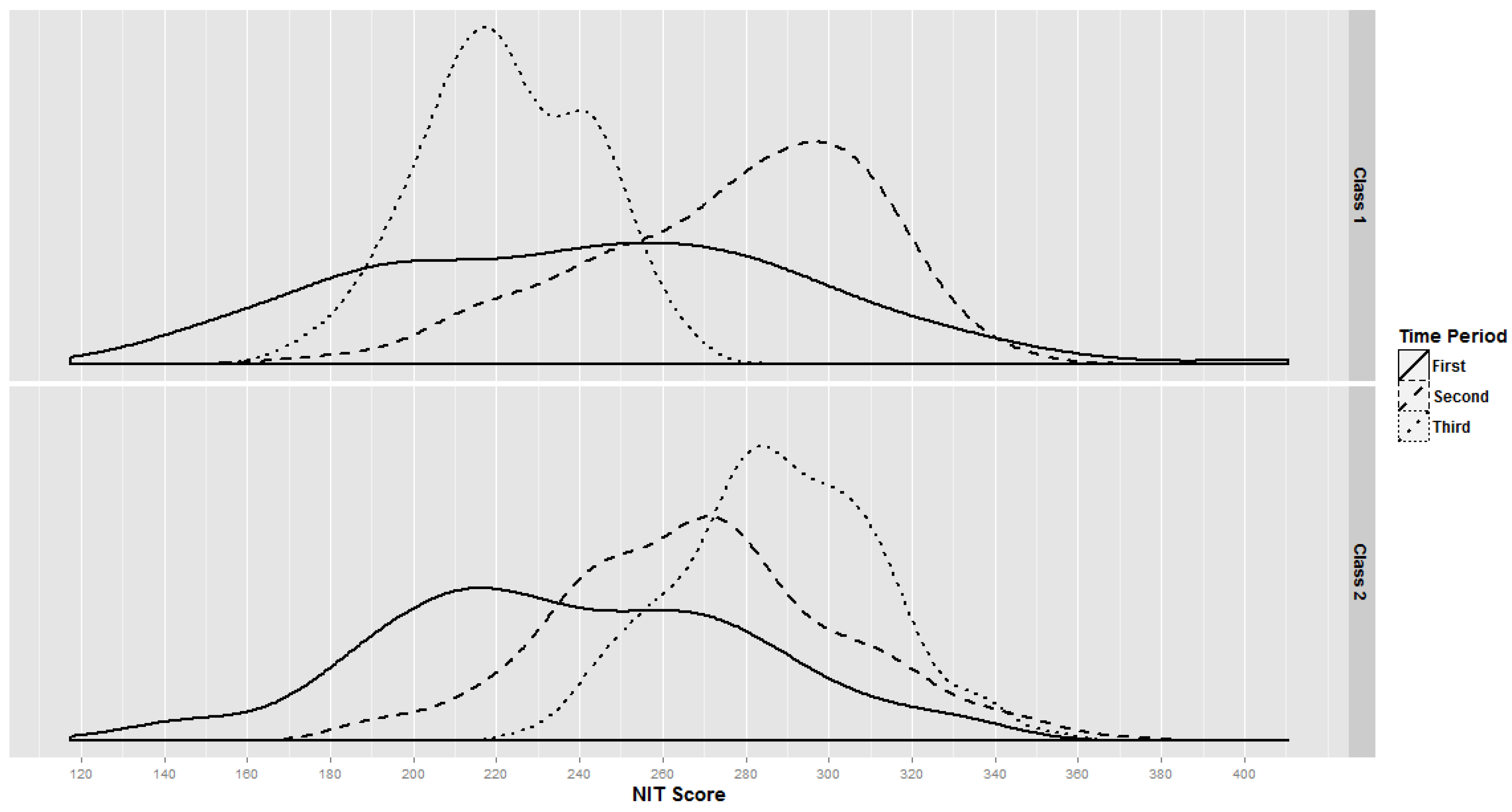
| Time 1 | 236.0 (49.4) | 238.2 (46.7) | 237.6 (47.3) |
| Time 2 | 266.4 (36.0) | 264.4 (36.1) | 264.9 (36.0) |
| Time 3 | 223.0 (19.4) | 287.9 (24.1) | 271.9 (36.2) |
| Fit Index | ||||||||
|---|---|---|---|---|---|---|---|---|
| Classes | AIC | AICc | CAIC | BIC | SSBIC | DIC | ICL-BIC | LMR p |
| 2 | 11,043 | 11,019 | 11,097 * | 11,086 * | 11,051 | 11,091 * | 11,301 * | 0.09 |
| 3 | 11,029 | 10,997 | 11,102 | 11,087 | 11,040 | 11,094 | 11,361 | 0.60 |
| 4 | 11,023 * | 10,983 | 11,116 | 11,097 | 11,036 * | 11,105 | 11,439 | 0.34 |
| 5 | 11,024 | 10,976 * | 11,136 | 11,113 | 11,040 | 11,124 | 11,544 | 0.49 |


4. Discussion
4.1. Design Factors
4.2. Consequences of Incorrect Model Selection
4.3. Additional Considerations
4.4. Comparison with Previous Flynn Effect Research Using the Estonian NIT
4.5. Recommendations
Author Contributions
Conflicts of Interest
References
- Flynn, J.R. What is Intelligence? Beyond the Flynn Effect; Cambridge University: New York, NY, USA, 2007. [Google Scholar]
- Flynn, J.R. Are We Getting Smarter? Rising IQ in the Twenty-first Century; Cambridge University Press: New York, NY, USA, 2012. [Google Scholar]
- Lynn, R. Who discovered the Flynn Effect? A review of early studies of the secular increase of intelligence. Intelligence 2013, 41, 765–769. [Google Scholar] [CrossRef]
- Williams, R.L. Overview of the Flynn effect. Intelligence 2013, 41, 753–764. [Google Scholar] [CrossRef]
- Rodgers, J.L. A critique of the Flynn Effect: Massive IQ gains, methodological artifacts, or both? Intelligence 1998, 26, 337–356. [Google Scholar] [CrossRef]
- Beaujean, A.A.; Osterlind, S.J. Using item response theory to assess the Flynn effect in the National Longitudinal Study of Youth 79 Children and Young Adults data. Intelligence 2008, 36, 455–463. [Google Scholar] [CrossRef]
- Wicherts, J.M.; Dolan, C.V.; Hessen, D.J.; Oosterveld, P.; van Baal, G.C.M.; Boomsma, D.I.; Span, M.M. Are intelligence tests measurement invariant over time? Investigating the nature of the Flynn effect. Intelligence 2004, 32, 509–537. [Google Scholar] [CrossRef]
- Beaujean, A.A.; Sheng, Y. Examining the Flynn effect in the general social survey vocabulary test using item response theory. Personal. Individ. Differ. 2010, 48, 294–298. [Google Scholar] [CrossRef]
- Shiu, W.; Beaujean, A.A.; Must, O.; te Nijenhuis, J.; Must, A. An item-level examination of the Flynn effect in Estonia. Intelligence 2013, 41, 770–779. [Google Scholar] [CrossRef]
- Pietschnig, J.; Tran, U.S.; Voracek, M. Item-response theory modeling of IQ gains (the Flynn effect) on crystallized intelligence: Rodgers’ hypothesis yes, Brand’s hypothesis perhaps. Intelligence 2013, 41, 791–801. [Google Scholar] [CrossRef]
- Cattell, R.B. The fate of national intelligence: Test of a thirteen-year prediction. Eugen. Rev. 1950, 42, 136–148. [Google Scholar] [PubMed]
- Shiu, W.; Beaujean, A.A. Evidence of the Flynn Effect in Children: A Meta-analysis. In Poster Presented at the Annual Meeting of the Association for Psychological Science, Boston, MA, USA; 2010. [Google Scholar]
- Shiu, W.; Beaujean, A.A. The Flynn Effect in Adults: A Meta-analysis. In Poster Presented at the Annual Meeting of the International Society for Intelligence Research, Arlington, VA, USA; 2010. [Google Scholar]
- Kanaya, T.; Ceci, S.J.; Scullin, M.H. Age differences within secular IQ trends: An individual growth modeling approach. Intelligence 2005, 33, 613–621. [Google Scholar] [CrossRef]
- Dolan, C.V.; van der Maas, H.L.J. Fitting multivariate normal finite mixtures subject to structural equation modeling. Psychometrika 1998, 63, 227–253. [Google Scholar] [CrossRef]
- Yung, Y.F. Finite mixtures in confirmatory factor-analysis models. Psychometrika 1997, 62, 297–330. [Google Scholar] [CrossRef]
- Bollen, K.A.; Curran, P.J. Latent Curve Models: A Structural Equation Perspective; Wiley: Hoboken, NJ, USA, 2006. [Google Scholar]
- Ram, N.; Grimm, K.J. Methods and measures: Growth mixture modeling: A method for identifying differences in longitudinal change among unobserved groups. Int. J. Behav. Dev. 2009, 33, 565–576. [Google Scholar] [CrossRef] [PubMed]
- Rodgers, J.L. The epistemology of mathematical and statistical modeling: A quiet methodological revolution. Am. Psychol. 2010, 65, 1–12. [Google Scholar] [CrossRef] [PubMed]
- Vermunt, J.K. The Sage Encyclopedia of Social Sciences Research Methods; Sage Publications: Thousand Oaks, CA, USA, 2004; chapter Latent profile model; pp. 554–555. [Google Scholar]
- Rodgers, J.L.; Rowe, D.C. Theory development should begin (but not end) with good empirical fits: A comment on Roberts and Pashler (2000). Psychol. Rev. 2002, 109, 599–603. [Google Scholar] [CrossRef] [PubMed]
- Bollen, K.A.; Long, J.S. (Eds.) Testing Structural Equation Models; Sage: Newbury Park, CA, USA, 1993.
- Tofighi, D.; Enders, C.K. Advances in Latent Variable Mixture Models; Information Age Publishing, Inc.: Greenwich, CT, USA, 2008; chapter Identifying the correct number of classes in growth mixture models; pp. 317–341. [Google Scholar]
- Beasley, W.H.; Rodgers, J.L. Bootstrapping and Monte Carlo methods. In APA Handbook of Research Methods in Psychology, Vol 2: Research Designs: Quantitative, Qualitative, Neuropsychological, and Biological; Cooper, H., Camic, P.M., Long, D.L., Panter, A.T., Rindskopf, D., Sher, K.J., Eds.; American Psychological Association: Washington, DC, USA, 2012; pp. 407–425. [Google Scholar]
- Fan, X. Designing simulation studies. In APA Handbook of Research Methods in Psychology (Vol. 3.): Data Analysis and Research Publication; Cooper, H., Ed.; American Psychological Association: Washington, DC, USA, 2012; pp. 427–444. [Google Scholar]
- Haggerty, M.E.; Terman, L.M.; Thorndike, R.L.; Whipple, G.M.; Yerkes, R.M. National Intelligence Tests: Manual of Directions; World Book: New York, NY, USA, 1920. [Google Scholar]
- Bandalos, D.L.; Leite, W. Structural Equation Modeling: A Second Course; Information Age Publishing: Charlotte, NC, USA, 2013; Chapter: Use of Monte Carlo studies in structural equation modeling research; pp. 625–666. [Google Scholar]
- Boomsma, A. Reporting Monte Carlo studies in structural equation modeling. Struct. Equ. Model. A Multidiscip. J. 2013, 20, 518–540. [Google Scholar] [CrossRef]
- Nylund, K.L.; Asparouhov, T.; Muthén, B.O. Deciding on the number of classes in latent class analysis and growth mixture modeling: A Monte Carlo simulation study. Struct. Equ. Model. 2007, 14, 535–569. [Google Scholar] [CrossRef]
- Kim, S.Y. Determining the Number of Latent Classes in Single-and Multiphase Growth Mixture Models. Struct. Equ. Model. 2014, 21, 263–279. [Google Scholar] [CrossRef] [PubMed]
- Singer, J.D.; Willett, J.B. Applied Longitudinal Data Analysis: Modeling Change and Event Occurrence; Oxford University: New York, NY, USA, 2003. [Google Scholar]
- Lipsey, M.W.; Hurley, S.M. Design sensitivity: Statistical power for applied experimental research. In The SAGE Handbook of Applied Social Research Methods; Bickman, L., Rog, D.J., Eds.; Sage: Thousand Oaks, CA, USA, 2009; pp. 44–76. [Google Scholar]
- McLachlan, G.J.; Peel, D. Finite Mixture Models; John Wiley & Sons, Inc.: New York, NY, USA, 2000. [Google Scholar]
- Collins, L.M.; Lanza, S.T. Latent Class and Latent Transition Analysis; John Wiley & Sons, Inc.: Hoboken, NJ, USA, 2010. [Google Scholar]
- Bollen, K.A. Structural Equation with Latent Variables; John Wiley & Sons, Inc.: New York, NY, USA, 1989. [Google Scholar]
- Lo, Y.; Mendell, N.R.; Rubin, D.B. Testing the number of components in a normal mixture. Biometrika 2001, 88, 767–778. [Google Scholar] [CrossRef]
- Vuong, Q.H. Likelihood ratio tests for model selection and non-nested hypotheses. Econometrica 1989, 57, 307–333. [Google Scholar] [CrossRef]
- Markon, K.E.; Krueger, R.F. An empirical comparison of information-theoretic selection criteria for multivariate behavior genetic models. Behav. Genet. 2004, 34, 593–610. [Google Scholar] [CrossRef] [PubMed]
- Muthén, B.O. LCA and Cluster Analysis. Message Posted to MPLUS Discussion List. Available online: http://www.statmodel.com/discussion/messages/13/155.html?1077296160 (accessed on 15 October 2013).
- Vermunt, J.K.; Magidson, J. Applied Latent Class Analysis; Cambridge University Press: Cambridge, MA, USA, 2002; Chapter: Latent class cluster analysis. [Google Scholar]
- Akaike, H. On the Entropy Maximization Principle; North-Holland: Amsterdam, The Netherlands, 1977; pp. 27–41. [Google Scholar]
- Bozdogan, H. Model selection and Akaike’s information criterion (AIC): The general theory and its analytical extensions. Psychometrika 1987, 52, 345–370. [Google Scholar] [CrossRef]
- Hurvich, C.M.; Tsai, C.L. Regression and time series model selection in small samples. Biometrika 1989, 76, 297–307. [Google Scholar] [CrossRef]
- Schwarz, G. Estimating the Dimension of a Model. Ann. Stat. 1978, 6, 461–464. [Google Scholar] [CrossRef]
- Sclove, S.L. Application of model-selection criteria to some problems in multivariate analysis. Psychometrika 1987, 52, 333–343. [Google Scholar] [CrossRef]
- Draper, D. Assessment and Propagation of Model Uncertainty. J. R. Stat. Soc. Ser. B (Methodological) 1995, 57, 45–97. [Google Scholar]
- Muthén, L.K.; Muthén, B.O. Mplus: User’s Guide, 6th ed.; Muthén & Muthén: Los Angeles, CA, USA, 2010; pp. 197–200. [Google Scholar]
- Celeux, G.; Soromenho, G. An entropy criterion for assessing the number of clusters in a mixture model. J. Classif. 1996, 13, 195–212. [Google Scholar] [CrossRef]
- Koehler, A.B.; Murphree, E.S. A comparison of the Akaike and Schwarz criteria for selecting model order. Appl. Stat. 1988, 41, 187–195. [Google Scholar] [CrossRef]
- Morgan, G.B. Mixed mode finite mixture modeling: An examination of fit index performance for classification. Struct. Equ. Model. in press.
- Soromenho, G. Comparing approaches for testing the number of components in a finite mixture model. Comput. Stat. 1994, 9, 65–82. [Google Scholar]
- Yang, C.C. Evaluating latent class analysis models in qualitative phenotype identification. Comput. Stat. Data Anal. 2006, 50, 1090–1104. [Google Scholar] [CrossRef]
- Celeux, G.; Soromenho, G. An entropy criterion for assessing the number of clusters in a mixture model. J. Classif. 1996, 13, 195–212. [Google Scholar] [CrossRef]
- Henson, J.M.; Reise, S.P.; Kim, K.H. Detecting mixtures from structural model differences using Latent variable mixture modeling: A comparison of relative model fit statistics. Struct. Equ. Model. 2007, 14, 202–226. [Google Scholar] [CrossRef]
- Ramaswamy, V.; DeSarbo, W.S.; Reibstein, D.J.; Robinson, W.T. An empirical pooling approach for estimating marketing mix elasticities with PIMS data. Mark. Sci. 1993, 12, 103–124. [Google Scholar] [CrossRef]
- Muthén, B.O. Mplus Technical Appendices, Version 3rd ed.; Muthén & Muthén: Los Angeles, CA, USA, 2004; pp. 197–200. [Google Scholar]
- Pastor, D.A.; Barron, K.E.; Miller, B.J.; Davis, S.L. A latent profile analysis of college students’ achievement goal orientation. Contemp. Educ. Psychol. 2007, 32, 8–47. [Google Scholar] [CrossRef]
- Biernacki, C.; Celeux, G.; Govaert, G. Assessing a mixture model for clustering with the integrated classification likelihood. In Technical Report; Institut National de Recherche en Informatique et en Automatique: Rhone-Alpes, France, 1998. [Google Scholar]
- McLachlan, G.J.; Ng, S.K. A comparison of some information criteria for the number of components in a mixture model. In Technical Report; Department of Mathematics, University of Queensland: Brisbane, Australia, 2000. [Google Scholar]
- Bento, C.; A., C.; Dias, G. (Eds.) Retails Clients Latent Segments, Proceedings of the 12th Portuguese Conference on Artificial Intelligence, Covilha, Portugal, 5–8 December 2005; Springer-Verlag: Heidelberg, Germany.
- Muthén, L.K.; Muthén, B.O. Mplus: User’s Guide, 7th ed.; Muthén & Muthén: Los Angeles, CA, USA, 2012. [Google Scholar]
- Hallquist, M.; Wiley, J. MplusAutomation: Automating Mplus Model Estimation and Interpretation; 2013; R Package Version 0.6-1. [Google Scholar]
- R Development Core Team. R: A Language and Environment for Statistical Computing; R Foundation for Statistical Computing: Vienna, Austria, 2013. [Google Scholar]
- Yerkes, R.M. Memoirs of the National Academy of Sciences: Psychological Examining in the United States Army; Government Printing Office: Washington, DC, USA, 1921; Volume 15. [Google Scholar]
- Must, O.; te Nijenhuis, J.; Must, A.; van Vianen, A.E.M. Comparability of IQ scores over time. Intelligence 2009, 37, 25–33. [Google Scholar] [CrossRef]
- Must, O.; Must, A.; Raudik, V. The secular rise in IQs: In Estonia, the Flynn effect is not a Jensen effect. Intelligence 2003, 31, 461–471. [Google Scholar] [CrossRef]
- Schaie, K.W. Quasi-experimental research designs in the psychology of aging. In Handbook of the Psychology of Aging; Birren, J.E., Schaie, K.W., Eds.; Van Nostrand Reinhold: New York, NY, USA, 1977; pp. 39–58. [Google Scholar]
- Peterson, R.A. A Meta-analysis of Cronbach’s coefficient alpha. J. Consum. Res. 1994, 21, 381–391. [Google Scholar] [CrossRef]
- Millsap, R.E. Structural equation modeling made difficult. Personal. Individ. Differ. 2007, 42, 875–881. [Google Scholar] [CrossRef]
- Bauer, D.J.; Curran, P.J. Distributional assumptions of growth mixture models: Implications for overextraction of latent trajectory classes. Psychol. Methods 2003, 8, 338–363. [Google Scholar] [CrossRef] [PubMed]
- McDonald, R.P. Structural models and the art of approximation. Perspect. Psychol. Sci. 2010, 5, 675–686. [Google Scholar] [CrossRef] [PubMed]
- Ang, S.C.; Rodgers, J.L.; Wänström, L. The Flynn effect within subgroups in the U.S.: Gender, race, income, education, and urbanization differences in the NLSY-Children data. Intelligence 2010, 38, 367–384. [Google Scholar] [CrossRef] [PubMed]
- Rodgers, J.L.; Wanstrom, L. Identification of a Flynn Effect in the NLSY: Moving from the center to the boundaries. Intelligence 2007, 35, 187–196. [Google Scholar] [CrossRef]
© 2014 by the authors; licensee MDPI, Basel, Switzerland. This article is an open access article distributed under the terms and conditions of the Creative Commons Attribution license (http://creativecommons.org/licenses/by/4.0/).
Share and Cite
Morgan, G.B.; Beaujean, A.A. An Investigation of Growth Mixture Models for Studying the Flynn Effect. J. Intell. 2014, 2, 156-179. https://doi.org/10.3390/jintelligence2040156
Morgan GB, Beaujean AA. An Investigation of Growth Mixture Models for Studying the Flynn Effect. Journal of Intelligence. 2014; 2(4):156-179. https://doi.org/10.3390/jintelligence2040156
Chicago/Turabian StyleMorgan, Grant B., and A. Alexander Beaujean. 2014. "An Investigation of Growth Mixture Models for Studying the Flynn Effect" Journal of Intelligence 2, no. 4: 156-179. https://doi.org/10.3390/jintelligence2040156