1. Introduction
Weyl semimetals (WSMs) constitute a remarkable example of three-dimensional, gapless materials with nontrivial topological properties—first proposed theoretically [
1,
2,
3,
4,
5,
6,
7] and, more recently, discovered experimentally on TaAs crystals [
8].
In a WSM, the band structure possesses an even number of Weyl nodes with linear dispersion, where the conduction and valence bands touch. These nodes are monopolar sources of Berry curvature, and hence are protected from being gapped since their charge (chirality) is a topological invariant [
7]. In the vicinity of these nodes, low energy conducting states behave as Weyl fermions, i.e., massless quasi-particles with pseudo-relativistic Dirac linear dispersion [
4,
5,
6,
7]. In Weyl fermions, conserved chirality determines the projection of spin over their momentum direction, a condition referred to as “spin-momentum locking”. While Type I WSMs are Lorentz covariant, this symmetry is violated in Type II WSMs, where the Dirac cones are strongly tilted [
9].
The presence of Weyl nodes in the bulk spectrum determines the emergence of Fermi arcs [
8], the chiral anomaly, and the chiral magnetic effect, among other remarkable properties [
9]. Therefore, considerable attention has been paid to understand the electronic transport properties of WSMs [
10,
11,
12]. For instance, there are recent works on charge transport [
13] in the presence of spin–orbit coupled impurities [
14], electrochemical [
15] and nonlinear transport induced by Berry curvature dipoles [
16]. Somewhat less explored are the effects of mechanical strain and deformations in WSMs. From a theoretical perspective, it has been proposed that different types of elastic strains can be modeled as gauge fields in WSMs [
17,
18,
19]. In previous works, we have studied the combined effects of a single torsional dislocation and an external magnetic field on the electronic [
20,
21] and thermoelectric [
20,
22] transport properties of WSMs, using the Landauer ballistic formalism in combination with a mathematical analysis for the quantum mechanical scattering cross-sections [
23].
In this work, we extend our previous analysis to study the case of a diluted, uniform concentration of torsional dislocations and its effects on the electrical conductivity of type I WSMs. In contrast to our former studies [
20,
21,
22], here we employ the Kubo linear-response formalism at finite temperatures. This requires explicitly calculating the retarded and advanced Green´s functions for the system, including the multiple scattering events due to the random distribution of dislocation defects in the form of a disorder-averaged self-energy term. For this purpose, we first analyze the scattering phase shift arising from a single torsional dislocation, and then we obtain the corresponding (retarded and advanced) Green’s function in terms of the T-matrix elements by solving analytically the Lippmann–Schwinger equation. We further extend this analysis, by incorporating the effect of a random distribution of such dislocations, with a concentration
, in the form of a disorder-averaged self-energy into the corresponding Dyson’s equation. Finally, we analyze the correction due to the scattering vertex, and by including this additional contribution, we calculate the electrical conductivity from the Kubo formula, as a function of temperature and concentration of dislocations. We present explicit evaluations of our analytical expressions for the electrical conductivity as a function of temperature and concentration of dislocations
, for several materials in the family of transition metals’ monopnictides, i.e., TaAs, TaP, NbAs and NbP, where the corresponding microscopic parameters, estimated by ab initio methods, were reported in the literature [
24,
25,
26].
2. Scattering by a Single Dislocation
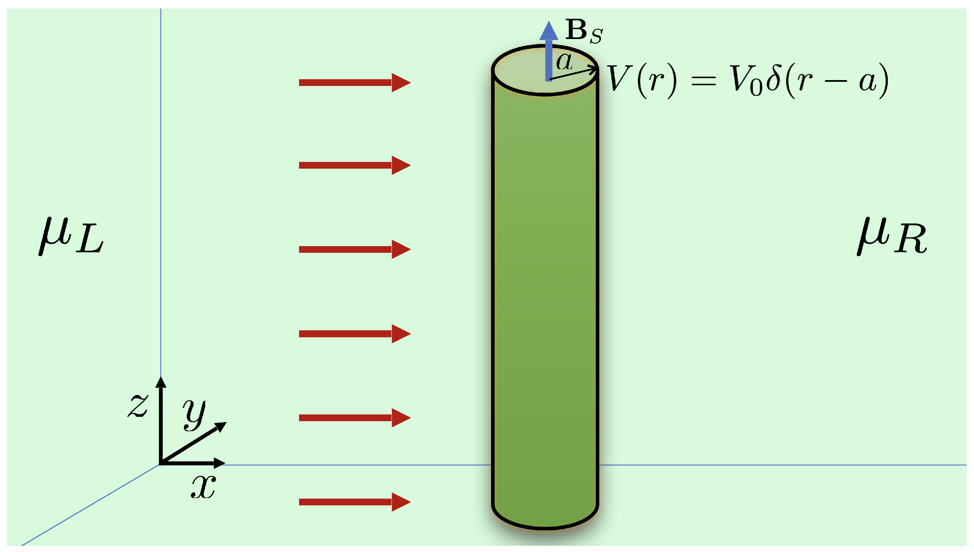
As a continuum model for a type I WSM under the presence of a single dislocation defect, as depicted in
Figure 1, we consider the Hamiltonian [
22]
where
Here,
labels each of the Weyl nodes located at
. The expression in Equation (
2) is the free-particle Hamiltonian, whereas the expression in Equation (
3) represents the interaction with the dislocation, where torsional strain is described as a pseudo-magnetic field inside the cylinder [
21,
22,
23], as well as the lattice mismatch effect at the boundary of the dislocation, modeled as a repulsive delta barrier on its surface [
22].
The “free” spinor eigenfunctions for the defect-free reference system satisfy
where the energy spectrum is given by
and
is the band (helicity) index. When projected onto coordinate space, these spinor eigenfunctions have the explicit form
and constitute an orthonormal basis for the Hilbert space.
If we now consider the (elastic) scattering effects induced by the torsional dislocation modeled by Equation (
3), we need to look for the eigenvectors
of the total Hamiltonian in Equation (
1) with the same energy as in Equation (
5). The answer is provided by the solution to the well-known Lippmann–Schwinger equation
where the free Green’s function can be expressed in a coordinate-independent representation form via the
resolvent,
Here, the index
stands for retarded and advanced, respectively. As shown in detail in
Appendix A, in the coordinate representation, the corresponding free Green’s function is given by the explicit matrix form
, where
and
Here, and are the Hankel functions, and is the position vector on any plane perpendicular to the cylinder’s axis.
For the scattering analysis, we need the retarded resolvent for the full Hamiltonian, which is defined as the solution to the equation
Combining Equation (
10) with Equation (
8), we readily obtain
where we introduced the standard definition of the T-matrix operator
that can be formally expressed in closed form by
Using this definition, along with the property
, we obtain the Lippmann–Schwinger Equation (
7) in the coordinate representation
As shown in detail in
Appendix B, by considering the asymptotic behavior of the Hankel functions,
(for
), Equation (
13) can be reduced to the
x–
y plane and takes the explicit asymptotic expression
where, as we explain in the
Appendix, the particles have only momenta perpendicular to the defect’s axis, i.e.,
. Comparing this last result with our previous reported expression for the scattering amplitude [
27],
we identify
. Therefore, we arrived at an explicit analytical expression for the T-matrix elements in terms of the phase shift
for each angular momentum channel
where
is the angle between
and
, and the analytical expression for the phase shift is given in
Appendix B by Equation (
A27).
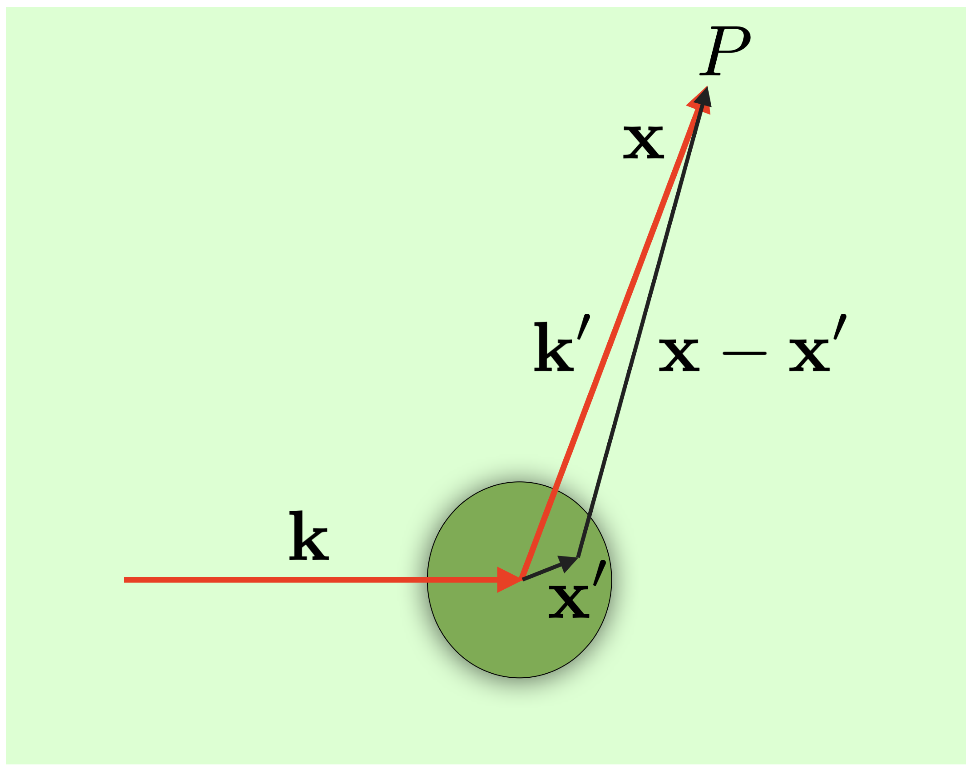
Figure 2.
Pictorial description of the scattering event on a plane perpendicular to the cylindrical defect axis.
Figure 2.
Pictorial description of the scattering event on a plane perpendicular to the cylindrical defect axis.
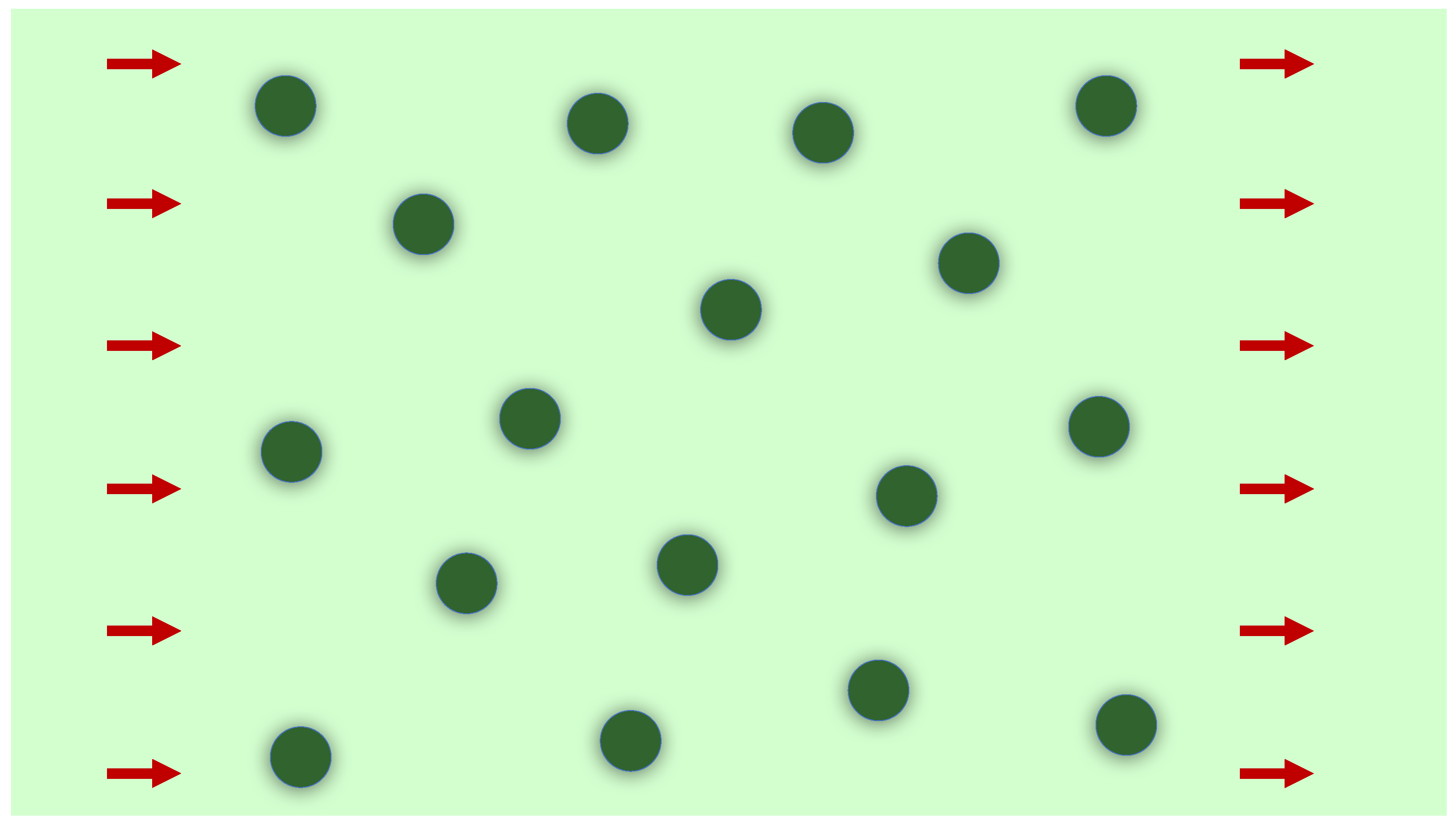
3. Scattering by a Uniform Concentration of Dislocations
Let us now consider a uniform concentration
(per unit transverse surface) of identical cylindrical dislocations, as depicted in
Figure 3, represented by the density function
where
is the position of the
-dislocation’s axis. The Fourier transform of this density function is thus given by the expression
The operator that plays the role of a scattering potential for this distribution of dislocation defects is
where
was defined in Equation (
3) as the contribution from a single dislocation. The matrix elements of the scattering operator Equation (
19) in the free spinor basis defined by Equation (
4) are
where
is the Fourier transform of
:
Then, the matrix elements of the potential in Equation (
20) become
Let us also introduce the configurational average of a function
over the statistical distribution of dislocations as
where
is the normalized distribution function for the defects in the sample. In particular, for a uniform distribution, we have
, where
A is the area of the plane normal to each cylinder’s axis. Now, the full retarded Green’s function under the presence of several dislocations represented by the operator
given in Equation (
19) satisfies the equation
The configurational average, as defined in Equation (
23), of the full Green’s function in this last equation can be written as
This is the Dyson’s equation with the retarded self-energy
that can be explicitly solved to yield
The effect of the statistical distribution of dislocations’ is entirely determined by the function
. In the perturbative expansion of the full Green’s function, we encounter
nth-products of the form
. The configurational average of a single factor is given by
Similarly, for the product of two factors, we obtain
and we have a similar behavior for higher order products. Now, notice that, for
, we have
,
and so on. We define the concentration of defects, i.e., the number of dislocations per unit of area perpendicular to the cylinder’s axis as
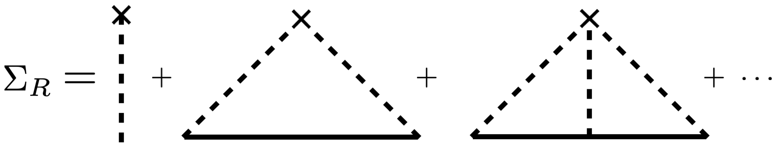
. As discussed in standard references [
28,
29], for small concentrations
, the scaling discussed before ensures that the total Green’s function in Equation (
25) can be calculated accurately by the sequence of diagrams for the retarded self-energy in momentum space as given in
Figure 4, an approach well known as the non-crossing approximation (NCA). This series of diagrams corresponds to the configurational average of the
T-matrix over the random distribution of dislocations after Equation (
23)
Using the expression in Equation (
16) for the
T-matrix elements, for
that implies
, we have that the real part of the self-energy
contains an infinite sum over highly oscillatory terms that converges to zero. Therefore, no contribution arises from the real part of the self-energy. The imaginary part, on the other hand, leads to the definition of the relaxation time,
3.1. Electrical Conductivity in the Linear-Response Regime
In order to arrive at the definition of the electrical conductivity in the linear response regime, let us first consider a single Fourier mode for an external electric field
, in the gauge
where
is the vector potential. Then,
. In the linear response formalism, the current is given by the expression
where the conductivity tensor is defined by
In the Kubo formalism, the tensor
is defined in terms of the retarded current-current correlator as follows:
where
is the statistical density matrix operator. As shown in detail in
Appendix D, the Fourier transform of this tensor to the frequency domain is given by
Here,
is the Fermi distribution, and we introduced the (disorder-averaged) spectral function
that clearly represents a Lorentzian distribution whose spectral width is defined by the inverse of the relaxation time (see
Appendix C for the details). After some algebraic manipulations, we obtain the conductivity tensor at finite frequency and temperature
Using the coordinates representation of the spectral function given in
Appendix C, after Equation (
A33), we can read off the Fourier transform to momentum space of the conductivity
We are interested in the DC conductivity, so we take the limit
first and then the limit
. After a long calculation (details in the
Appendix D), the result is
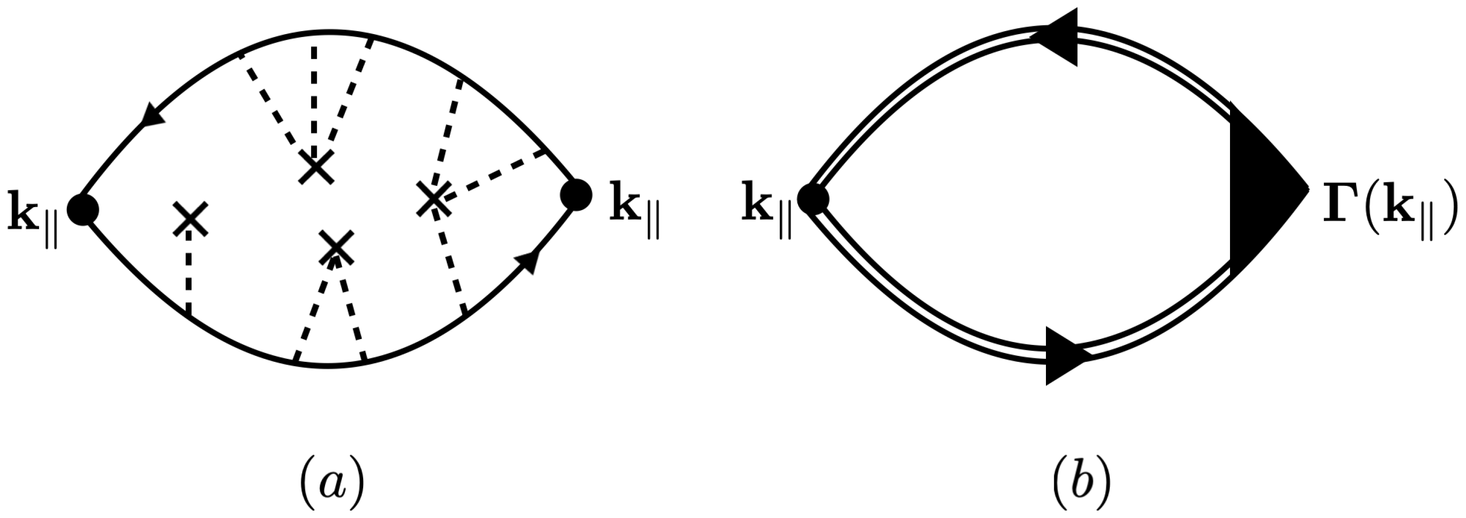
3.2. Vertex Corrections
The self-energy contribution modifies the definition of the retarded and advanced Green´s functions in Equation (
40), as depicted by the double lines in
Figure 5b. However, there are also scattering processes involving links between the two internal Green function lines, as depicted in
Figure 5a. When considering such diagrams with cross-links, as in
Figure 5a, we must include the vertex correction as depicted in
Figure 5b.
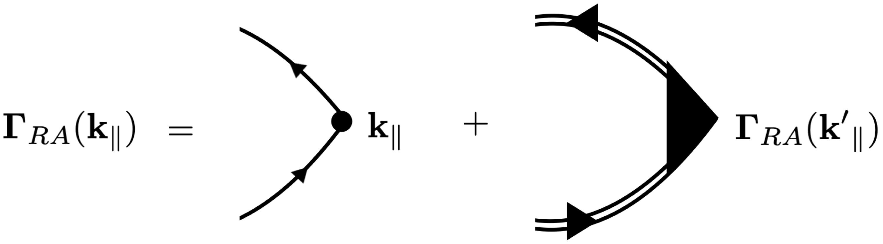
Taking into account the vertex correction, the conductivity becomes
where the vertex function
is given as the solution to the
Bethe-Salpeter equation as depicted in
Figure 6. Then, we have
The iterative solution of Equation (
42) for
shows that the vertex function must be of the form
Then, we obtain a secular integral equation for the scalar function
that in the low concentration limit becomes
In the limit of low concentrations, we use the result in
Appendix D, Equation (
A46), to obtain
At low temperatures, an exact solution is possible since the derivative of the Fermi distribution takes a compact support at the Fermi energy. Therefore, we can evaluate
and
at the Fermi momentum
, to obtain
where we defined (for
)
After the substitution of
from Equation (
46) into Equation (
45), we finally obtain a closed analytical expression for the bulk electrical conductivity, as a function of temperature and concentration of dislocations
where
is the polylogarithm of order 2. Here, the total
transport relaxation time is defined by
Using the analytical expression for the
T-matrix elements in Equation (
16), we obtain a closed expression for the transport relaxation time in terms of the scattering phase shifts
From Equation (
48), we can investigate the zero temperature
and high temperature
limits, respectively. In the zero temperature limit, we obtain
a constant that depends on the microscopic material properties (such as
), as well as on the concentration of dislocations
through the relaxation time.
On the other hand, in the high-temperature limit
, we obtain a quadratic dependence on temperature
where the overall constant depends on the microscopic parameters for each material, as well as on the concentration of dislocations through the relaxation time.
4. Results
In this section, we apply the theory and analytical expressions obtained in the previous section to calculate the electrical conductivity of several materials in the family of transition metals’ monopnictides, i.e., TaAs, TaP, NbAs, and NbP. For an estimation of the concentration of defects
in real crystal systems, Ref. [
24] reports that the native concentration of dislocations in the lattice of the materials TiO
2 and SrTiO
3 varies in the range
–
. These concentrations can be enhanced using different treatments up to
, close to the rendering amorphous limit. The microscopic/atomistic parameters involved in our theory are obtained from
ab-initio studies for WSM materials, as reported in Refs. [
25,
26]. In particular, the later reference identifies anisotropies in the Fermi velocities and density of charge carries at different Weyl nodes and bands. Using these results for the densities of carriers, we compute the Fermi momentum at each Weyl node, i.e.,
, as displayed in
Table 1.
In what follows, for definiteness, we shall assume that the axis of the defects is along the crystallographic
z-direction and that we are measuring the conductivity along the
x-direction. Then, we use the reported
x-components of the Fermi velocities [
25,
26]. We have different Fermi velocities
, for the conduction band (
) and for the valence band (
), and for each of the Weyl nodes (
), respectively. Actually, for the valence band, Refs. [
25,
26] report the
hole velocity. Their results are presented in
Table 2.
Now, in order to study the additional effect of the torsional dislocations, we follow our previous work [
22] to estimate the geometrical parameters involved in the model. We assume that the dislocations are cylindrical regions along the
z-axis with radius
a. Here, we further assume that the defects possess an average radius of
nm. The simple relation between the torsional angle
(in degrees) and the pseudo-magnetic field representing strain is
[
22], where the modified flux quantum in this material is approximately
. In this work, we have chosen a torsion angle
. The lattice mismatch effect at the surface of the dislocation cylinders is modeled by a repulsive delta-potential, with strength
, expressed in terms of the “spinor rotation” angle
. According to our previous work [
22], a realistic choice is
.
With all of these parameters fixed, we can compute the transport relaxation time for each material from Equation (
50). Our results are presented in
Table 3.
Now, we compute the conductivity along the
x-direction
. In what follows, we simply call it
, as a function of temperature. The total conductivity is the sum over nodes and bands
where
is given in Equation (
48), including the vertex correction. Our results for
are presented in
Table 4.
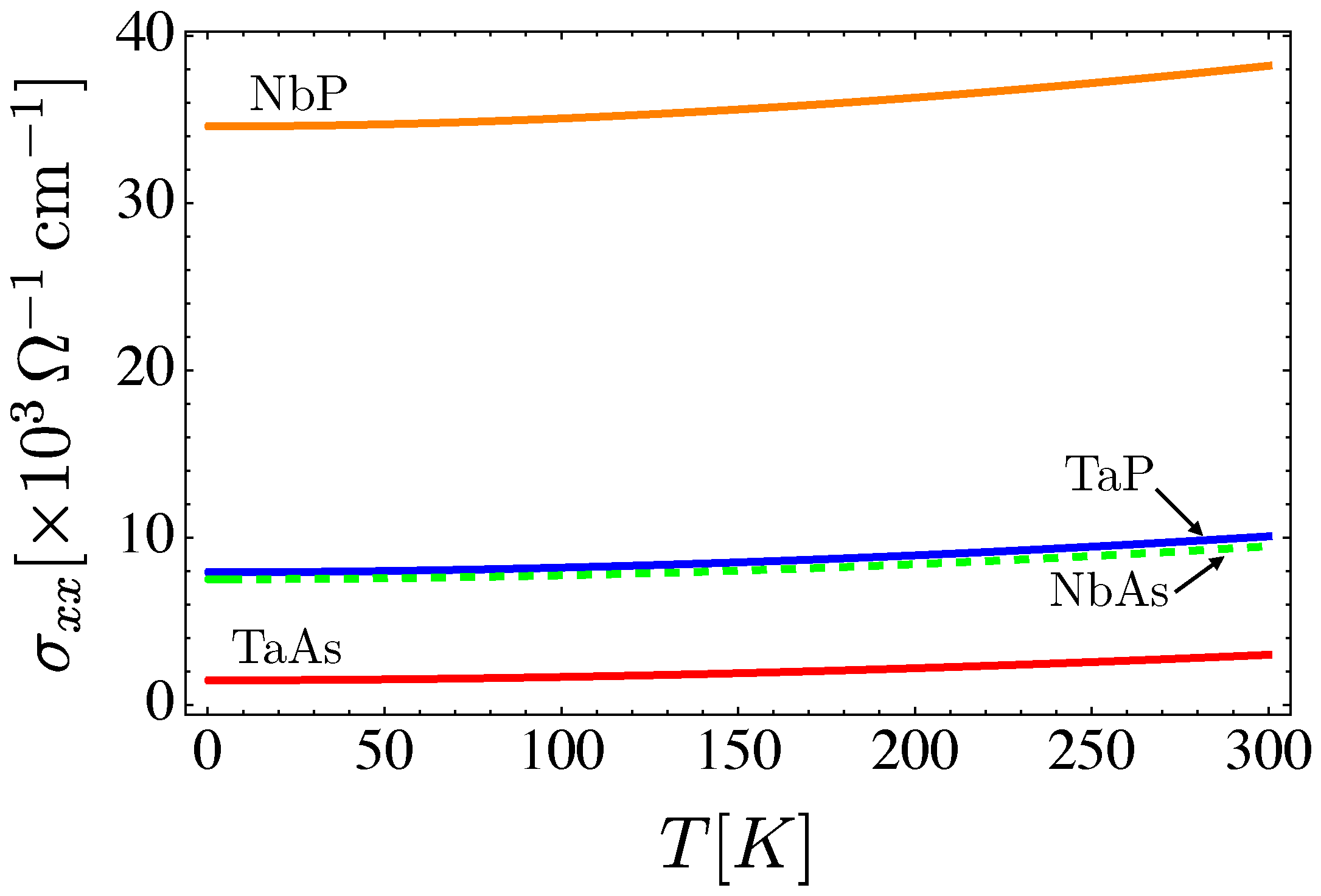
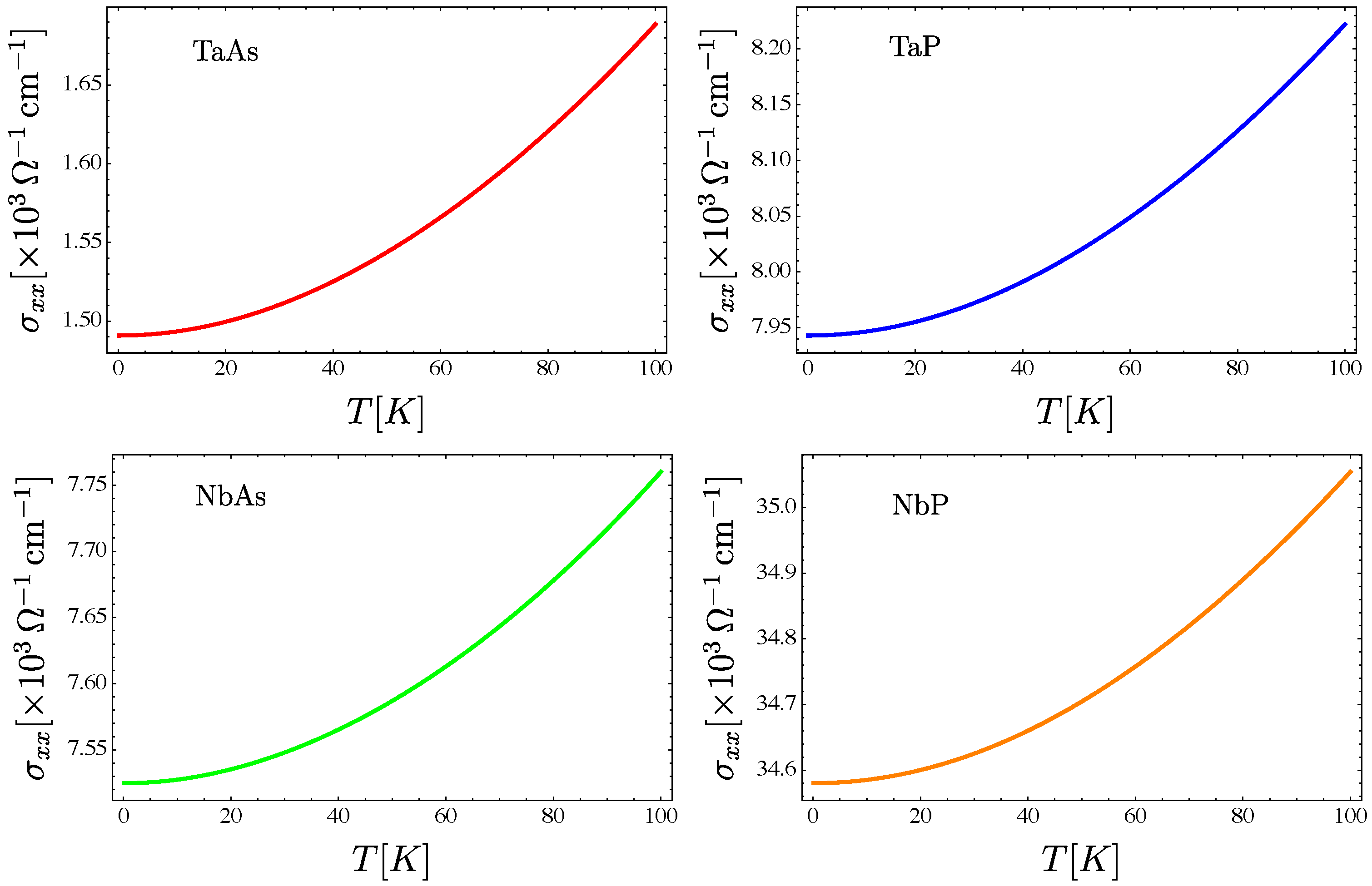
The conductivity as a function of temperature, for the transition metals’ monopnictides TaAs, TaP, NbAs and NbP, is presented in
Figure 7 for all of them compared, and individually in the panel
Figure 8.
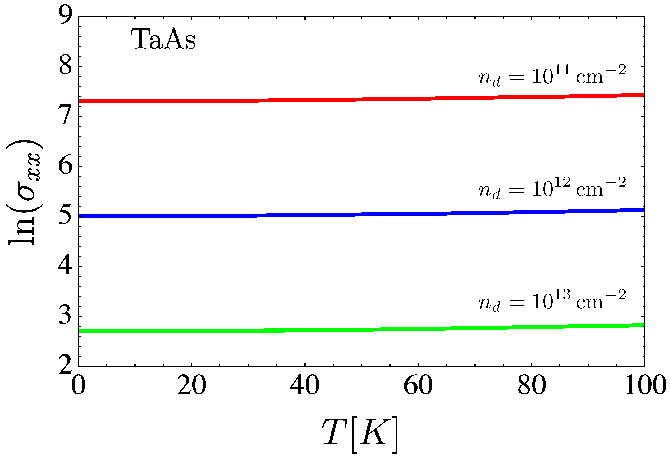
Now, let us study the conductivity behavior with respect to the density of dislocations
. In
Figure 9, we present a plot of the natural logarithm of the conductivity versus temperature for three different concentrations of dislocations.
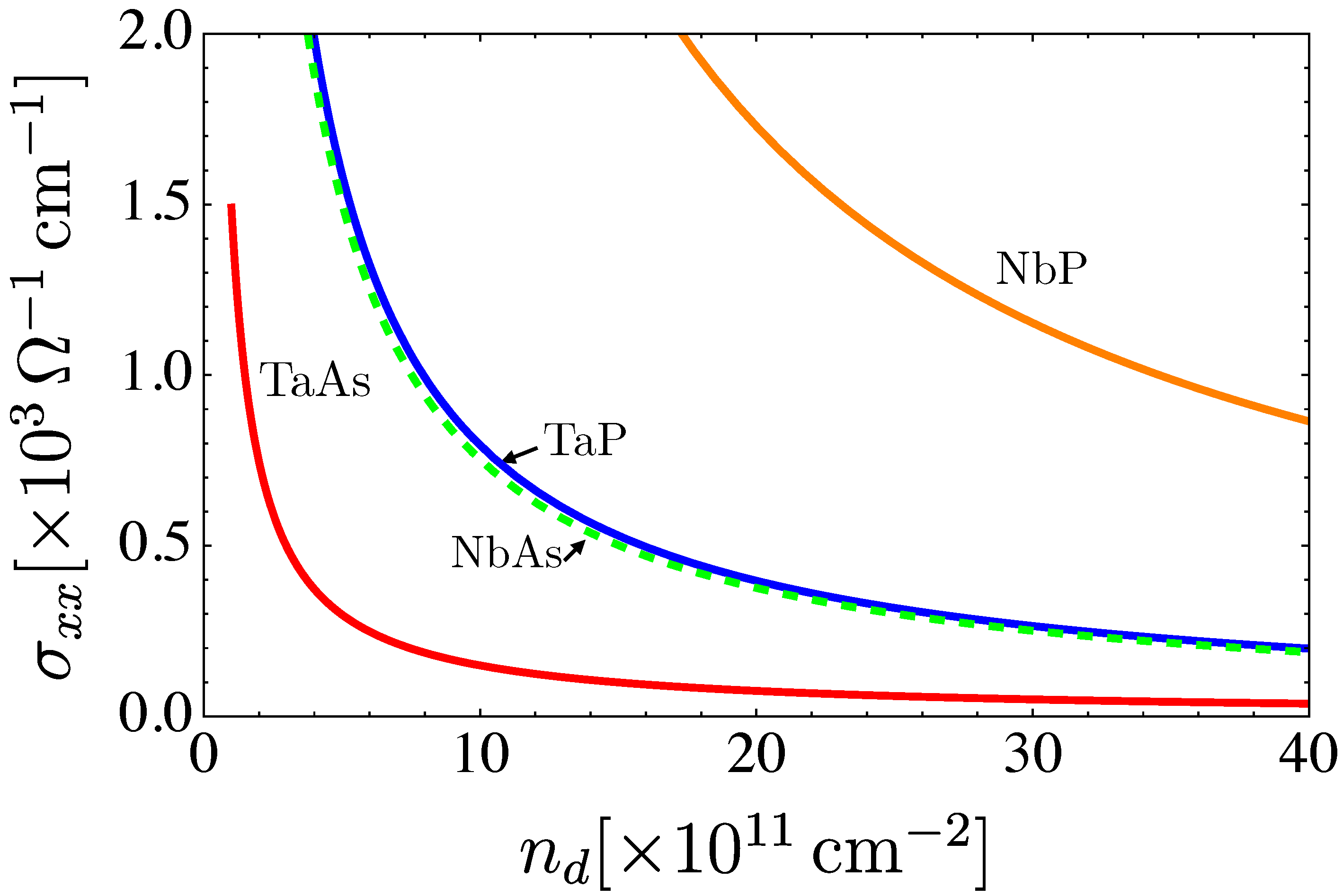
The total conductivity as a function of the concentration of defects and at zero temperature is presented in
Figure 10.
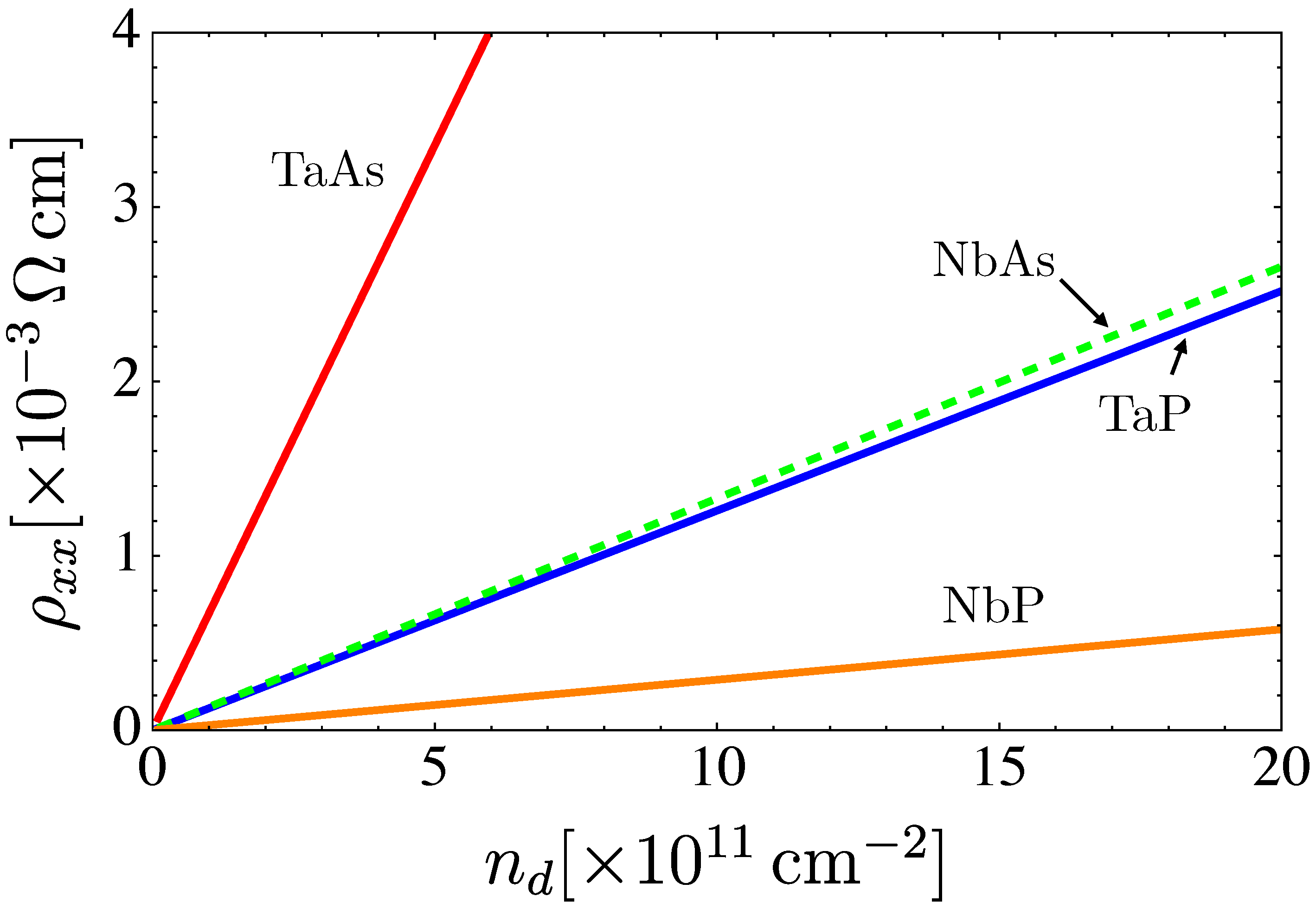
Finally, a plot of the resistance, defined as the inverse of conductivity, as a function of the dislocations’ density is presented in
Figure 11.
5. Discussion and Conclusions
In this work, we have studied the effect of a distribution of mechanical defects, i.e., torsional dislocations, over the electrical conductivity of the family of transition metals monopnictides TaAs, TaP, NbAs and NbP. Our theory is based on the mathematical analysis of the scattering phase shifts from a single defect, as stated in our previous work [
20,
21,
22,
23,
27]. We extended this previous analysis to develop a Green´s function formalism, in order to represent the scattering due to a finite concentration of randomly distributed defects. Within the non-crossing approximation for the self-energy, we solved explicitly for the disorder-averaged retarded Green´s function that allows us to calculate the electrical conductivity in the Kubo linear-response formalism. We obtained general analytical expressions in terms of the parameters involved in the low-energy model representing the family of materials, and using the
ab-initio estimations for such parameters, we provided a characterization of the conductivity as a function of temperature and concentration of defects for the transition metal monopnictides TaAs, TaP, NbAs and NbP. As a universal feature, we identified a
temperature dependence for
, where the pre-factor depends on material-specific microscopic parameters as well as in the concentration of dislocations
through the scattering relaxation time. Our results do not involve the electron–phonon scattering effects that will presumably contribute at finite temperatures. However, those can be included via Mathiessen’s rule in an overall relaxation time combining Equation (
50) for
with a separate theoretical estimation for the electron–phonon relaxation time
, as follows:
. Since the electron–phonon interaction that determines the magnitude of
is an entirely different physical mechanism, it deserves an analysis on its own, to be communicated in a separate article which is under current development.


