Pattern Recognition of Neurotransmitters: Complexity Reduction for Serotonin and Dopamine


 and
and
Abstract
1. Introduction
2. Material
2.1. Reagents
2.2. Equipment
2.3. Data Collection
3. Methods
3.1. Data Preprocessing
3.2. Experimental Implementation
3.3. Feature Reduction
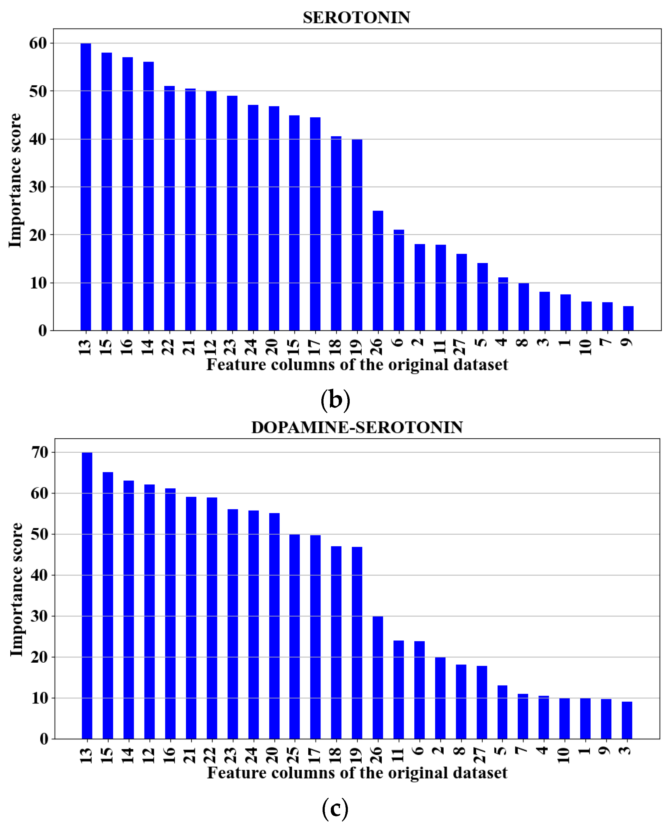
3.4. Further Feature Reduction
3.5. Framework of the Experiments
4. Results
5. Comparison with Other Works
- Sazanova et al. [1] used seven principal components and seven latent variables from the original data for application in the traditional pattern recognition techniques, PCR and PLSR, respectively. Their models detected and predicted the concentrations of DA alone and SE alone in in vitro mixtures. They obtained a test accuracy ranges for correct classifications of 42–62% for DA and 33–50% for SE. To increase the ranges of these accuracies, they extended the ranges for correct prediction to include one level above and below the true concentration level, obtaining new accuracy ranges of 81–91% for DA and 91–100% for SE. This extension of levels increased the confidence interval for the estimation of the NTs, deviating from the “true” concentration estimates for the NTs in the mixtures. We thus believe that simultaneously detecting and predicting the “true” concentration levels of DA and SE in vitro with the modified PCR and PLSR, i.e., PCA-GPR and PLS-GPR models respectively, yields better results than detecting and predicting the concentrations of the NTs separately.
- Movassaghi et al. [2] applied rapid pulse voltammetry wave forms coupled with PLSR (RPV-PLSR) using a smart pulse approach for the simultaneous monitoring of DA and SE for in vitro and in vivo complex environments across time scales. The work included background current in NT monitoring and used 518 latent variables to train the PLSR models to construct their in vitro model. These steps caused overfitting, as argued by [23,24,25,26]. Further, they used a moving average kernel to map each latent variable to low, medium, or high correlation using the shading technique, ranging from 0 to 100% shading. This step assimilated the voltage-dependent current-response data to be time-series data without applying the guidelines stated by [26] for the conversion of any data to time-series data. We thus demonstrated that it is possible to select subsets of predictors to reduce the complexities and time required for NT detection and prediction, hence avoiding any conversion of the data structure by using GPR, which efficiently fills the spaces between data points through interpolation to generate continuous representations [18].
6. Validation
7. Discussion
8. Conclusions
Author Contributions
Funding
Institutional Review Board Statement
Informed Consent Statement
Data Availability Statement
Conflicts of Interest
References
- Sazonova, N.; Njagi, J.; Marchese, Z.; Ball, M.; Andreescu, S.; Schuckers, S. Detection and prediction of concentrations of neurotransmitters using voltammetry and pattern recognition. In Proceedings of the Annual International Conference of the IEEE Engineering in Medicine and Biology Society, Minneapolis, MN, USA, 3–6 September 2009; pp. 3493–3496. [Google Scholar]
- Movassaghi, C.S.; Perrotta, K.A.; Yang, H.; Iyer, R.; Cheng, X.; Dagher, M.; Fillol, M.A.; Andrews, A.M. Simultaneous serotonin and dopamine monitoring across timescales by rapid pulse voltammetry with partial least squares regression. Anal. Bioanal. Chem. 2021, 413, 6747–6767. [Google Scholar] [PubMed]
- Hoseok, C.; Shin, H.; Cho, H.U.; Blaha, C.D.; Heien, M.L.; Yoonbae, O.; Lee, K.H.; Jang, D.P. Neurochemical concentration prediction using deep learning vs principal component regression in fast scan cyclic voltammetry: A comparison study. ACS Chem. Neurosci. 2022, 13, 2288–2297. [Google Scholar]
- Cooper, J.R.; Bloom, F.E.; Roth, R.H. The Biochemical Basis of Neuropharmacology, 8th ed.; Oxford Univ. Press: Oxford, UK, 2002. [Google Scholar]
- Kapur, S.; Remington, G. Serotonin-dopamine interaction and its relevance to schizophrenia. Amer. J. Psychiatry 1996, 153, 466–476. [Google Scholar]
- Mathur, R.; Pathak, V.; Bandil, D. Parkinson Disease Prediction Using Machine Learning Algorithm; Springer Nature Singapore Pte Ltd.: Singapore, 2019. [Google Scholar]
- Vitek, J.L.; Jain, R.; Chen, L.; Tröster, A.I.; Schrock, L.E.; House, P.A.; Giroux, M.L.; Hebb, A.O.; Farris, S.M.; Whiting, D.M.; et al. Subthalamic nucleus deep brain stimulation with a multiple independent constant current-controlled device in Parkinson’s disease (INTREPID): A randomized, double-blind, sham-controlled study. Lancet Neurol. 2020, 19, 491–501. [Google Scholar] [CrossRef]
- Follett, K.A.; Weaver, F.M.; Stern, M.; Hur, K.; Harris, C.L.; Luo, P.; Marks, W.J., Jr.; Rothlind, J.; Sagher, O.; Moy, C.; et al. Pallidal versus subthalamic deep-brain stimulation for Parkinson’s disease. N. Engl. J. Med. 2010, 362, 2077–2091. [Google Scholar] [CrossRef] [PubMed]
- Williams, A.; Gill, S.; Varma, T.; Jenkinson, C.; Quinn, N.; Mitchell, R.; Scott, R.; Ives, N.; Rick, C.; Daniels, J.; et al. Deep brain stimulation plus best medical therapy versus best medical therapy alone for advanced Parkinson’s disease (PD SURG trial): A randomised, open-label trial. Lancet Neurol. 2010, 9, 581–591. [Google Scholar] [CrossRef] [PubMed]
- Si, B.; Song, E. Recent advances in the detection of neurotransmitters. Chemosensors 2018, 6, 1. [Google Scholar] [CrossRef]
- Thenaisie, Y.; Palmisano, C.; Canessa, A.; Keulen, B.J.; Capetian, P.; Jiménez, M.C.; Bally, J.F.; Manferlotti, E.; Beccaria, L.; Zutt, R.; et al. Towards adaptive deep brain stimulation: Clinical and technical notes on a novel commercial device for chronic brain sensing. J. Neural Eng. 2021, 18, 042002. [Google Scholar] [CrossRef] [PubMed]
- Njagi, J.; Chernov, M.M.; Leiter, J.C.; Andreescu, S. Amperometric detection of dopamine in vivo with an enzyme-based carbon fiber microbiosensor. Anal. Chem. 2010, 82, 989–996. [Google Scholar] [CrossRef] [PubMed]
- Chauhan, N.; Soni, S.; Agrawal, P.; Balhara YP, S.; Jain, U. Recent advancement in nanosensors for neurotransmitters detection: Present and future perspective. Process Biochem. 2020, 91, 241–259. [Google Scholar]
- Singh, A.; Sharma, A.; Ahmed, A.; Sundramoorthy, A.K.; Furukawa, H.; Arya, S.; Khosla, A. Recent advances in electrochemical biosensors: Applications, challenges, and future scope. Biosensors 2021, 11, 336. [Google Scholar] [CrossRef] [PubMed]
- Stefan-van Staden, R.-I.; Moldoveanu, I.; van Staden, J.F. Pattern recognition of neurotransmitters using multimode sensing. J. Neurosci. Methods 2014, 229, 1–7. [Google Scholar] [CrossRef] [PubMed]
- Pakchin, P.S.; Nakhjavani, S.A.; Saber, R.; Ghanbari, H.; Omidi, Y. Recent advances in simultaneous electrochemical multi-analyte sensing platforms. TrAC Trends Anal. Chem. 2017, 92, 32–41. [Google Scholar] [CrossRef]
- Schoors, J.V.; Viaene, J.; Van Wanseele, Y.; Smolders, I.; Dejaegher, B.; Heyden, B.V.; Van Eeckhaut, A. An improved microbore UHPLC method with electrochemical detection for the simultaneous determination of low monoamine levels in in vivo brain microdialysis samples. J. Pharm. Biomed. Anal. 2016, 127, 136–146. [Google Scholar] [PubMed]
- Manzhos, S.; Ihara, M. Rectangularization of Gaussian process regression for optimization of hyperparameters. Mach. Learn. Appl. 2023, 13, 100487. [Google Scholar] [CrossRef]
- Kim, J.; Oh, Y.; Park, C.; Kang, Y.M.; Shin, H.; Kim, I.Y.; Jang, D.P. Comparison study of partial least squares regression analysis and principal component analysis in fast-scan cyclic voltammetry. Int. J. Electrochem. Sci. 2019, 14, 5924–5937. [Google Scholar] [CrossRef]
- Hyoung, D.K.; Oh, Y.; Shin, H.; Blaha, C.D.; Bennet, K.E.; Lee, K.H.; Kim, I.; Jang, D.P. Investigation of the reduction process of dopamine using paired pulse voltammetry. J. Electroanal. Chem. 2014, 717, 157–164. [Google Scholar]
- Igene, L.; Alim, A.; Imtiaz, M.H.; Schuckers, S. A machine learning model for early prediction of Parkinson’s disease from wearable sensors. In Proceedings of the IEEE 13th Annual Computing and Communication Workshop Conference, virtual, 8–11 March 2023. [Google Scholar]
- Giordano, G.F.; Ferreira, L.F.; Bezerra, Í.R.; Barbosa, J.A.; Costa, J.N.; Pimentel, G.J.; Lima, R.S. Machine learning toward high-performance electrochemical sensors. Anal. Bioanal. Chem. 2023, 415, 3683–3692. [Google Scholar] [CrossRef] [PubMed]
- Apon, H.J.; Abid, M.S.; Morshed, K.A.; Nishat, M.M.; Faisal, F.; Moubarak, N.N.I. Power system harmonics estimation using hybrid Archimedes optimization algorithm-based least square method. In Proceedings of the 13th International Conference on Information & Communication Technology and System (ICTS), Surabaya, Indonesia, 20–21 October 2021. [Google Scholar]
- Kabir, M.R.; Muhaimin, M.M.; Mahir, M.A.; Nishat, M.M.; Faisal, F.; Moubarak, N.N.I. Procuring MFCCs from Crema-D dataset for sentiment analysis using deep learning models with hyperparameter tuning. In Proceedings of the IEEE International Conference on Robotics, Automation, Artificial-Intelligence and Internet-of-Things (RAAICON), Dhaka, Bangladesh, 3–4 December 2021. [Google Scholar]
- Rahman, A.A.; Siraji, M.I.; Khalid, L.I.; Faisal, F.; Nishat, M.M.; Islam, M.R.; Moubarak, N.N.I. Detection of mental state from EEG signal data: An investigation with machine learning classifiers. In Proceedings of the 14th International Conference on Knowledge and Smart Technology (KST), Chonburi, Thailand, 26–29 January 2022. [Google Scholar]
- Jahangiri, A.; Rakha, H.A. Applying machine learning techniques to transportation mode recognition using mobile phone sensor data. IEEE Trans. Intell. Transp. Syst. 2015, 16, 2406–2417. [Google Scholar] [CrossRef]
- Moubarak, N.N.I.; Omar, N.M.M.; Youssef, V.N. Smartphone-sensor-based human activities classification for forensics: A machine learning approach. J. Electr. Syst. Inf. Technol. 2024, 11, 33. [Google Scholar]


| Experiment Number | Training Sets (with 10-Fold Cross-Validation) | Testing Set (Independent Set) |
|---|---|---|
| Exp 1 | 1 and 2 | 3 |
| Exp 2 | 1 and 3 | 2 |
| Exp 3 | 2 and 3 | 1 |
| Dataset Feature Voltages | Training and Testing | Accuracy | R2 Values |
|---|---|---|---|
| DA | |||
| All features −0.16 V to 0.88 V | TR | 87.6 | 0.75 |
| TE | 87.6 | 0.77 | |
| OPW features 0 V to 0.52 V | TR | 86.2 | 0.72 |
| TE | 87.6 | 0.78 | |
| SE | |||
| All features −0.16 V to 0.88 V | TR | 88.0 | 0.72 |
| TE | 88.1 | 0.74 | |
| OPW features 0 V to 0.52 V | TR | 87.3 | 0.70 |
| TE | 87.9 | 0.74 | |
| DA–SE | |||
| All features −0.16 V to 0.88 V | TR | 96.7 | 0.76 |
| TE | 96.7 | 0.77 | |
| OPW features 0 V to 0.52 V | TR | 96.4 | 0.73 |
| TE | 96.5 | 0.77 | |
| Dataset Feature Voltages | Training and Testing | Accuracy | R2 Values |
|---|---|---|---|
| DA | |||
| All features −0.16 V to 0.88 V | TR | 88.2 | 0.77 |
| TE | 87.3 | 0.77 | |
| OPW features 0 V to 0.52 V | TR | 87.7 | 0.76 |
| TE | 86.8 | 0.77 | |
| SE | |||
| All features −0.16 V to 0.88 V | TR | 88.5 | 0.71 |
| TE | 83.8 | 0.58 | |
| OPW features 0 V to 0.52 V | TR | 87.7 | 0.78 |
| TE | 85.0 | 0.65 | |
| DA–SE | |||
| All features −0.16 V to 0.88 V | TR | 96.8 | 0.77 |
| TE | 95.1 | 0.60 | |
| OPW features 0 V to 0.52 V | TR | 96.8 | 0.78 |
| TE | 95.4 | 0.66 | |
| NT | Columns of Subset from Original Dataset | Training and Testing | Accuracy | R2 Value |
|---|---|---|---|---|
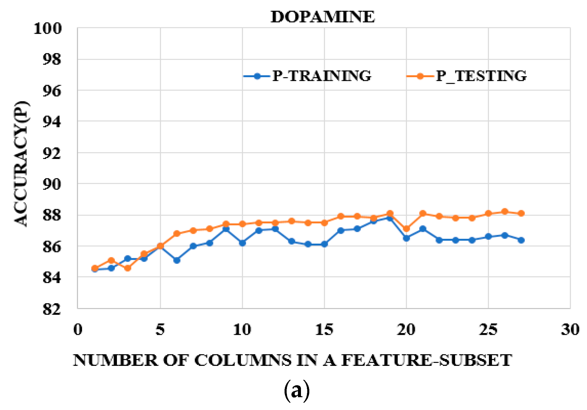
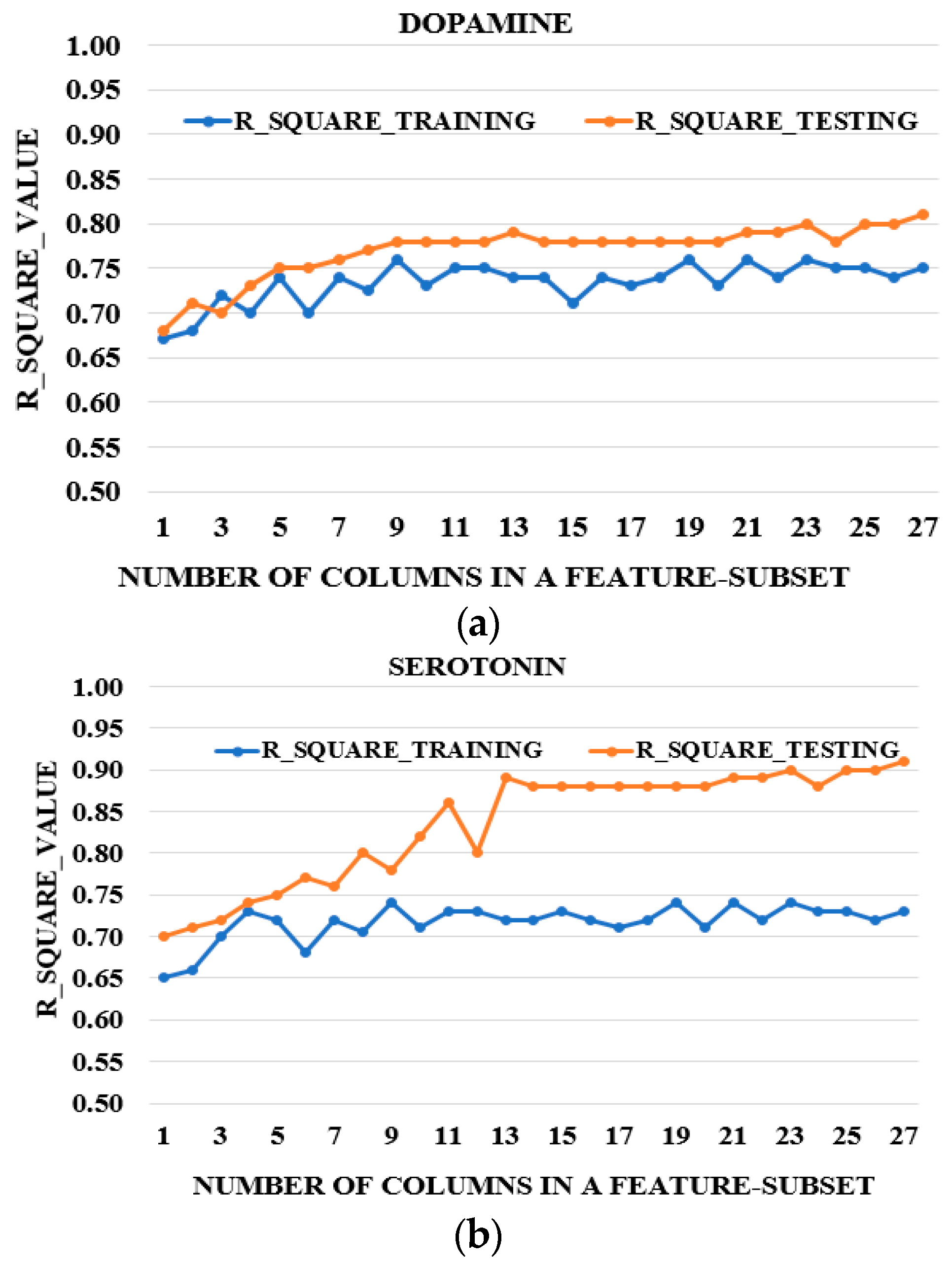
| DA | 9, 8, 10, 11, 7 | TR TE | 86.73 86.76 | 0.75 0.756 |
| SE | 13, 15, 16, 14 | TR TE | 87.83 87.93 | 0.74 0.743 |
| DA–SE | 13, 15, 14, 12, 16 | TR TE | 97.41 97.4 | 0.75 0.743 |
| NT | Columns of Subset from Original Dataset | Training and Testing | Accuracy | R2 Value |
|---|---|---|---|---|
| DA | 9, 8, 10, 11, 7 | TR TE | 83.73 82.76 | 0.74 0.75 |
| SE | 13, 15, 16, 14 | TR TE | 86.83 87.93 | 0.76 0.73 |
| DA–SE | 13, 15, 14, 12, 16 | TR TE | 95.42 96.3 | 0.74 0.73 |
Disclaimer/Publisher’s Note: The statements, opinions and data contained in all publications are solely those of the individual author(s) and contributor(s) and not of MDPI and/or the editor(s). MDPI and/or the editor(s) disclaim responsibility for any injury to people or property resulting from any ideas, methods, instructions or products referred to in the content. |
© 2025 by the authors. Licensee MDPI, Basel, Switzerland. This article is an open access article distributed under the terms and conditions of the Creative Commons Attribution (CC BY) license (https://creativecommons.org/licenses/by/4.0/).
Share and Cite
Nchouwat Ndumgouo, I.M.; Devoe, E.; Andreescu, S.; Schuckers, S. Pattern Recognition of Neurotransmitters: Complexity Reduction for Serotonin and Dopamine. Biosensors 2025, 15, 209. https://doi.org/10.3390/bios15040209
Nchouwat Ndumgouo IM, Devoe E, Andreescu S, Schuckers S. Pattern Recognition of Neurotransmitters: Complexity Reduction for Serotonin and Dopamine. Biosensors. 2025; 15(4):209. https://doi.org/10.3390/bios15040209
Chicago/Turabian StyleNchouwat Ndumgouo, Ibrahim Moubarak, Emily Devoe, Silvana Andreescu, and Stephanie Schuckers. 2025. "Pattern Recognition of Neurotransmitters: Complexity Reduction for Serotonin and Dopamine" Biosensors 15, no. 4: 209. https://doi.org/10.3390/bios15040209
APA StyleNchouwat Ndumgouo, I. M., Devoe, E., Andreescu, S., & Schuckers, S. (2025). Pattern Recognition of Neurotransmitters: Complexity Reduction for Serotonin and Dopamine. Biosensors, 15(4), 209. https://doi.org/10.3390/bios15040209