Abstract
Rough surfaces are in contact locally by the peaks of roughness. At this local scale, the pressure of contact can be sharply superior to the macroscopic pressure. If the roughness is assumed to be a random morphology, a well-established observation in many practical cases, mechanical indicators built from the contact zone are then also random variables. Consequently, the probability density function (PDF) of any mechanical random variable obviously depends upon the morphological structure of the surface. The contact pressure PDF, or the probability of damage of this surface can be determined for example when plastic deformation occurs. In this study, the contact pressure PDF is modeled using a particular probability density function, the generalized Lambda distributions (GLD). The GLD are generic and polymorphic. They approach a large number of known distributions (Weibull, Normal, and Lognormal). The later were successfully used to model damage in materials. A semi-analytical model of elastic contact which takes into account the morphology of real surfaces is used to compute the contact pressure. In a first step, surfaces are simulated by Weierstrass functions which have been previously used to model a wide range of surfaces met in tribology. The Lambda distributions adequacy is qualified to model contact pressure. Using these functions, a statistical analysis allows us to extract the probability density of the maximal pressure. It turns out that this density can be described by a GLD. It is then possible to determine the probability that the contact pressure generates plastic deformation.
1. Introduction
Surface integrities has been a growing field over the last 30 years. During contact, stress can induce fractures, scratches and micro-cracks influencing operational life, secular stability and coating quality [1,2,3,4]. Rough surfaces are locally and sparsely in contact, essentially at roughness peaks. At this specific scale, the contact pressure can be sharply superior to the apparent or macroscopic pressure. In numerous practical cases, the roughness is a random morphology. So it becomes obvious to integrate the surface morphology as a random process to compute the local pressures as a probability density function (PDF). Then, the probability of damage on the surface can also be computed from macroscopic material properties. Greenwood pioneered the first rough contact model in 1966 [5] on a pure elastic contact to explain that the real area of contact between asperities can be proportional to the load. One advantage of this model is that it becomes possible to measure macroscopic features taking account some roughness parameters measurements. The rough surface is presented as a set of uncorrelated rough peaks with spherical tips of constant radius of curvature. Thus, for each asperity, Hertz’s theories can be then applied. Greenwood assumed that the heights of the asperities varied randomly with known PDF without lack of generality but analyzed analytically and numerically the exponential and Gaussian PDFs. In his paper, roughness estimators used to compute these PDFs and PDF itself are considered as perfectly known i.e., adequation between the theoretical model fit perfectly with experimental data and estimator are supposedly known, meaning that there are calculated one an infinite surface. These two strong assumptions are intensively used in all modelling on rough surfaces (optics, mechanics, thermal, biology…). However, four years after this pioneering work, Greenwood treated the problems of the first contact point of an asperity [6]. A sentence written marginally by Greenwood is of major interest: “… Some arguments arise from confusion between a sample and a population…” and points to the problems of sampling variations. For the first time (in Appendix A of Greenwood’s publication) the extreme values theory is applied but restricted to the case when estimators of the parent distribution are perfectly known. Different distributions are discussed and the role of the spread of the distribution emphasised. It is pointed in this article that the first contact determination is experimentally a difficult task due to the lack of knowledge’s of the reference point. About the remarks of T. R. Thomas, R. M. Baul and W. Scott, Greenwood recognized that more experimental evidence is needed on the tails of height distributions to settle the question of whether heights are truly Gaussian or not. In 1972, Tsakada et al. [7] introduce a method to determine the highest point of ground surfaces (the extreme value of surface roughness). As pointed by the authors, the probability density function of surface asperity has always been assumed to be a normal distribution. However, Tsakada showed the Weibull distribution gives a better approximation to characterize the extreme value of rough surfaces and estimate experimentally that the extreme value of surface asperity coincides with the value calculated by the Weibull distribution that represent one of the extreme statistics of PDF. Curiously, since Tsakada’s article, it has become difficult over nearly four decades (1970–2010) to find in the bibliography an article presenting the relationships between extreme values of roughness and the problematic of contact mechanics. In 2009, Zwol et al. [8] showed that the point at which two random rough surfaces in a plate-plate contact takes place at the contact of the highest asperities and has a crucial importance for determination of dispersive forces. This uncertainty depends on the roughness of interacting bodies but authors no not used extreme values theory to model this effect. In 2012, Broer et al. [9] used explicity extreme values statistics to calculate the Casimir force at separations linked to the root-mean square of the height fluctuations of the two rough surfaces. Applied on gold samples, they showed the presence of peaks considerably higher than the root-mean-square roughness. These peaks redefine the minimum separation distance between the bodies and can be described by extreme value statistics. Ponthus et al. [10] show that the statistical properties of the normal motion’s amplitude are well captured by a simple analytic model based on the extreme value theory framework, extending its applicability to sliding-contact-related topics. A complete analysis of extreme values applied on friction between rough surfaces is undertaken by Melekan and Rouhani [11]. They proposed a model based on extreme value statistics and combine it with different models for single-asperity contact, including adhesive and elasto-plastic contacts, to derive a relation between the applied load and the friction force on a rough interface. They show that extreme values probabilities of peak asperities can better fit the contact features of Greenwood models, closest to Amonton’s law.
2. Materials and Methods
2.1. Simulation of Rough Surfaces
In a first step, surfaces are simulated using Weierstrass functions. A set of real surfaces are created presenting a wide range of surfaces met in tribology [12,13]. The three dimensional fractal Weierstrass surfaces are defined as [14]:
where and are stochastic phases of uniform density defined in [0, 2π].
A is a scale coefficient, are normal random numbers, H is the Hölder exponent (), is the frequency of the function with .
The functions plotting for fractal dimension i.e., are shown in Figure 1.

Figure 1.
Simulated surfaces (1024 × 1024) following Weierstrass distribution with three different Hurst exponents (1, ½, 0) from left to right.
2.2. Semi-Analytical Model
In this approach, a rough hard surface is in contact with a perfectly smooth rigid plane. In this case, local contacts are localized at the surface peaks. We consider the approximation of geometric contacts where elastic deformation between asperities is neglected.
2.2.1. Conical Model of Roughness
The roughness is modeled by a succession of indenters with a distribution of attack angles. Each asperity is described by a cone with a hemispherical end tip. The definition of the average deformation is introduced by taking into account the average attack angle of the roughness . The indentation by an axi-symmetrical indenter allows estimating the stresses and strains applied in the indented material. For conical tip geometry [15], the mean pressure is related to the attack angle β of the tip. Following the pressure supported by the summit, we can distinguish three regimes of deformation. In the case of an elastic contact, the mean pressure (mp) undergone by the asperity can be written [16]:
where E* stands for the combined Young’s modulus of the two surfaces in contact given by , Ej and νj are respectively the Young modulus and the Poisson’ ratio relative to surface j.
pm = 0.2 E*tan β
2.2.2. Solution Procedure
The local behavior of each asperity is investigated numerically by the analysis of the local peak geometry. The local area of the contact Aj between an asperity j and the plane is assumed elliptic, having semi-axes aj and bj, Aj is given by:
For numerical purpose, the local area Aj is discretized into N elements cji (i = 1, 2, … N). The local pressure distribution on each asperity j, is given by:
where pjm is the mean pressure associated with asperity j. The normal force Fj exerted on the asperity j is given by the following relation:
The total load supported by summits is thus:
where m is the total number of asperities in contact.
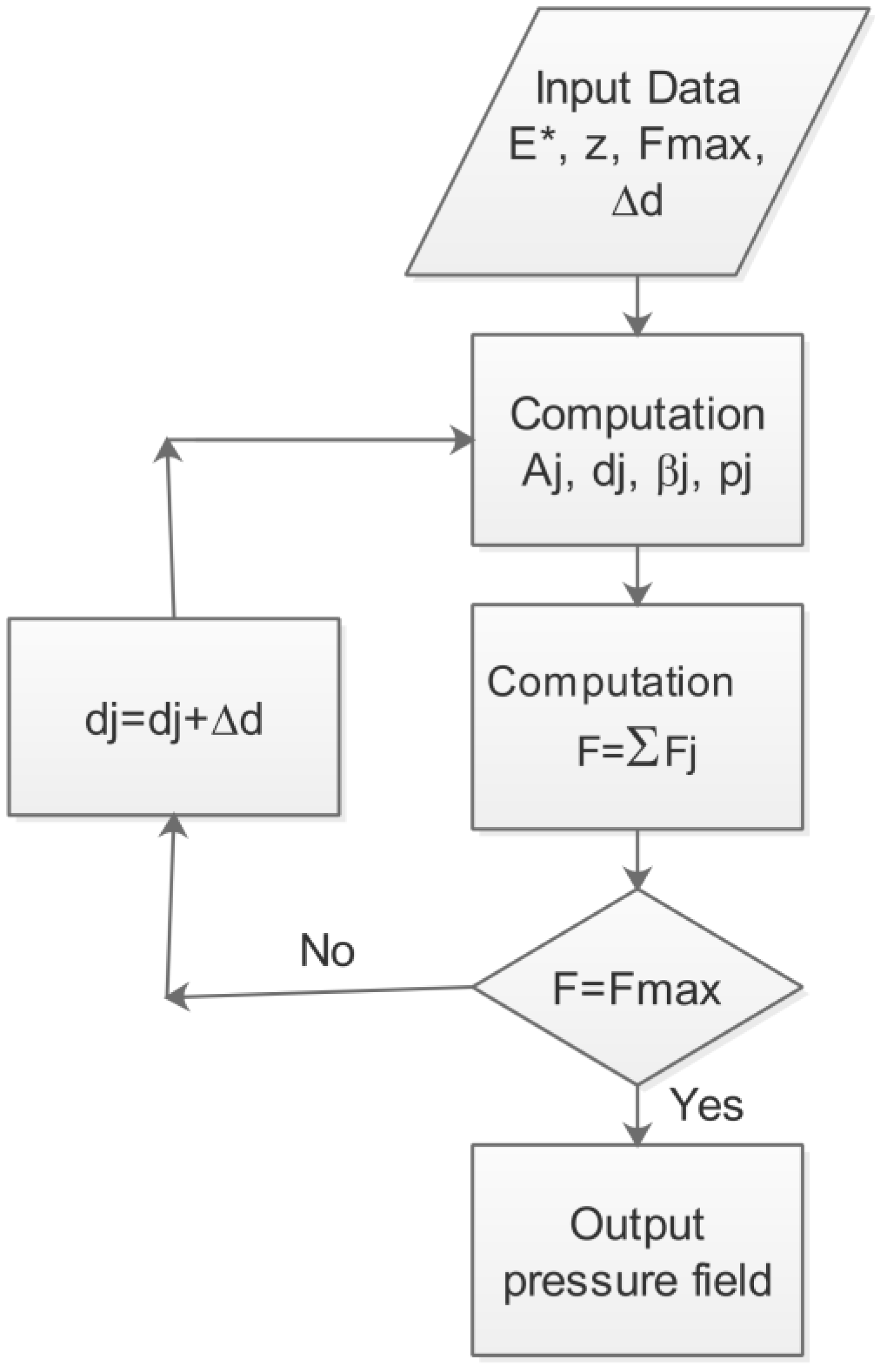
Figure 2 is a flowchart for the contact calculation program. The three-dimensional surface topography is directly sampled by the computer-generated surface topography.

Figure 2.
Flowchart for the numerical calculation of the pressure field.
The surface topography is characterised by N × M points. Each point of the coordinates (x,y) has a height z. Data are saved in binary format and are used as input for a three dimensional surface topology detection algorithm [17,18]. The latter is used to determine the position and the peak of each asperity. For each point i located at (xi,yi) of amplitude zi (denoted by zi(xi,yi)), the difference Δz(xi,yi) = zi(xi,yi) − z(xs,yr) is calculated and compared to the heights of the eight neighboring points in the Cartesian grid where s = i − 1, i, i + 1 and r = j − 1, j, j + 1. If all Δz(xi,yi) > 0, z(xi,yj) will be regarded as the asperity peak.
For a given initial separation d, the local displacement dj, the local contact area Aj, and the average attack angle βj of each asperity can be determined. These parameters allow the distribution of the pressure and the real contact area undergone by the roughness to be determined. For a macroscopic displacement, the two surfaces are progressively brought to contact with several displacement increments Δd of the smooth rigid plane. The displacement is interrupted when the resulting effort F reaches the imposed normal effort FMAX (i.e., the convergence of the numerical software is reached).
2.2.3. Pressure Distribution
The model is applied on the three surfaces defined on Figure 1. The macroscopic pressure is equal to Pm = 20 MPa, using Young modulus E = 210 GPa. Surface are normalized such with their r.m.s. roughness Rq = 50 µm on a 1 mm² surfaces discretized over 1024 points in each direction. Figure 3 represents the pressure distribution for the three surfaces, respectively, described in the Figure 1.

Figure 3.
Results of the pressure distribution for the three surfaces described in Figure 1 with 3 Hurst exponents.
3. Results
3.1. Probability Density Functions (PDFs)
As described in the introduction, the pressure is stochastic. Its PDF depends on the roughness’s PDF. In our case, we decide to directly model the pressure without taking account directly the roughness in the computation. Taking the pressure map, pressure distribution is supposed to be stationary in the spatial scale. This means that peaks morphology do not depends on space in average. Under these conditions, the probability density function do not depends on positions x and y and thus becomes one-dimensional. However this probability density function can be split into two parts. Let α be the probability to meet a zero pressure (no contact) then the probability of meeting a non-zero pressure is equals to 1 − α. The PDF can be written:
is the Dirac function localized on p = 0, and G(p) is the PDF associated with continuous non zero pressure.
In practice, only G(p) is required to compute the contact pressure. Moreover, primary hypotheses linked to spatial homogeneity of date are problematic to evaluate. Furthermore, the selection of PDF is frequently associated to the authors’ modelling backgrounds or the suitability of the PDF to adjust adequately the data under study. Moreover, the retained distributions are poorly compared between others distributions and rarely checked by statistical tests of goodness of fit. In this paper, the maximum pressure PDF, a major interest in contact mechanics, will be modelled which is why the statistics of the extreme value theory will be applied. However, the application of classical extreme value analysis could have significant limits. As the most commonly used Gumbel and Generalized Extreme Value (GEV) methods [19] include inferred parental PDF constrained by mathematical assumptions, we suggest another way to circumvent the need for a priori hypothesis.
Our approach is a combination of the Generalized Lambda Distribution (GLD) and the Computer-Based Bootstrap Method (CBBM). Unlike the Gumbel and GEV models, which incorporate the statistical properties of the parent PDF, the GLD and the CBBM both have the common benefit of bypassing the preconceived choice of a well-known theoretical PDF that would approximate the physics of contact mechanisms.
It should be noted that GLD’s are extremely flexible due to their capacity to adopt a wide spectrum of shapes, including common unimodal distributions. GLD’s are defined by four parameters and can thus correspond to the first four moments of the experimental data (mean, variance, asymmetry, kurtosis) and also include asymptotic properties on the extreme values (tails extended to infinity or truncated, on either or both sides).
In the field of surface integrities, there are a multitude of known statistical distributions that model, using more or less well-founded simplifying assumptions, the damage mechanisms. For example, the normal law is often used to model static mechanical properties (stiffness, plasticity), Weibull’s laws for cumulative damage mechanisms (fatigue, corrosion), lognormal laws the distribution of defects (porosity density), Gumbel’s law the distribution of critical defects (pitting), Pareto’s law the fracture values at interfaces (toughness) and all these distributions are well model by GLD [20,21]. The quality of fit obtained with the GLD’s is especially notable in the region of the right tail of the empirical PDF, which is of interest to the extreme values of the pressure distribution described in this paper. For several years, one of the author of the present paper has been developing the use of this flexible family of PDF in the field of Materials Science [22,23,24] and also in Statistical Process Control [25,26].
The principle of statistical modelling of extreme contact pressures is a four-step process. In the first step, the distribution of contact pressures is modelled by the semi-analytical model for calculating local pressures corresponding to an experimental distribution of n pressure values. In a second step, a bootstrap (CBBM) is applied to generate a large number of k sets of n pressure data. In a third step, k GLD are modeled from the k*n bootstrapped data. Finally (step 4), for each of the k GLD, the extreme values are estimated and the histogram of extreme values (probability density of extreme values) is constructed. From this empirical density, the mean of the maximum pressure and a 90% confidence interval can be estimated.
3.1.1. Basic Concept
The GLD family is specified in terms of its inverse distribution function with four parameters (λ1, λ2, λ3 and λ4):
The parameters λ1 and λ2 are, respectively, the location and scale parameters, while λ3 and λ4 are related respectively to the skewness and the kurtosis of the GLD with 0 ≤ y ≤ 1 (see [25,26] for details). The PDF is obtained from the inverse distribution function of Equation (8):
where y is the solution of the equation QX(y) = x which can be solved numerically.
Equation (9) defines a valid PDF if and only if QX meets the following conditions:
where D is the domain of definition of QX.
3.1.2. Numerical Estimation of Pressure PDF
An algorithm was developed using the Statistical Analyses System (SAS) language to compute the GLD parameters from an experimental dataset (in our study, moment method is used). Applied on the pressure described on Figure 3, the value of λ1, λ2, λ3, λ4 are computed from the four moment estimators , , , (Table 1).

Table 1.
Values of the fourth moments and the generalized Lambda distribution (GLD) parameters for the three pressure corresponding to the Hurst exponent of H = 0, 0.5 and 1 (Figure 3).
Figure 4 presents the PDF of the GLD corresponding to the PDF of contact pressure computed from surface topography (Figure 3, Table 1). GLD fits very well contact pressure computed from experimental surface topography.

Figure 4.
Plots of the GLD probability density functions and empirical histograms parameters for the three local pressures corresponding to the Hurst exponent of H = 0, 0.5 and 1.
3.1.3. Bootstrap Protocol
Efron [27,28] introduced first the Computer-Based Bootstrap Method (CBBM) to avoid the risk of asserting wrong conclusions when analysing experimental data that transgress inference assumptions of the traditional statistical theory. A main reason for making parametric assumptions is to facilitate the derivation from textbook formulae for standard errors. Based on the mathematical resampling technique, the main principle of the CBBM consists in generating a high number B of simulated bootstrap samples from the original data points. The original dataset consists of either experimental or simulated points. A bootstrap dataset of pressures of size n, noted (p*1, p*2, …, p*n), is a collection of n values simply obtained by randomly sampling with replacement from the original pressure data (p1, p2, …, pn), each of them with a probability of 1/n. The bootstrap dataset thus consists of elements of the original data points; some appearing zero times, some appearing once, some twice, etc.
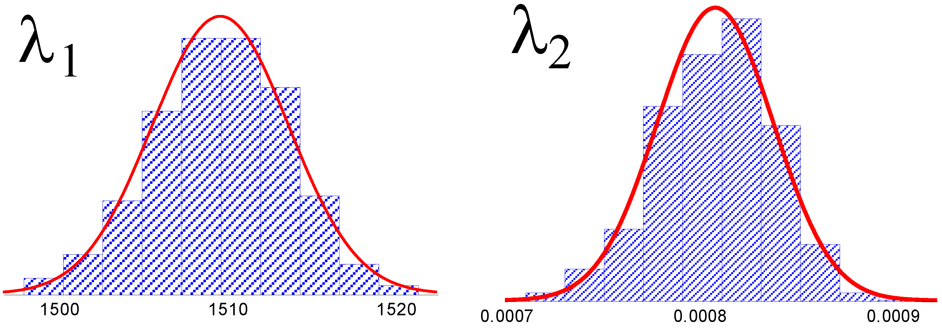
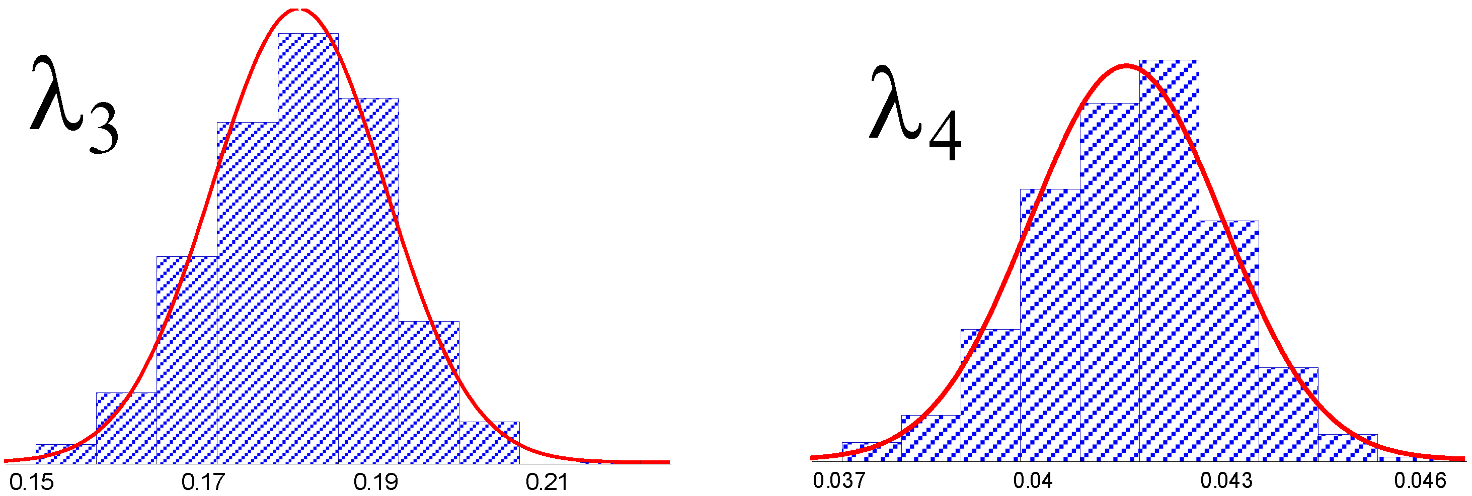
Applied on the surface H = 0.5, probability density functions of Lambda coefficients can be plotted (Figure 5).
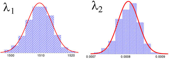
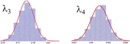
Figure 5.
Plots of the probability density functions of the four GLD parameters obtained from 1000 bootstraps for the Hurst exponent of H = 0.5.
3.2. Maximal Pressure Probability Density Functions
3.2.1. Formulation
The density function, Pmax, of the maximal pressure distribution corresponding to the GLD (Equation (8)) is given by the inverse distribution function of this distribution, Qmax:
With density function, f is:
where Q’ is the derivative of Q and F the cumulative distribution function (CDF) of the Q PDF (i.e., F = Q−1). Thus, the Pmax function is evaluated for any pressure value x by numerically inverting the Qmax function as well as the density function Pmax. To plot the Pmax function, one first computes the quantile function QX with set of y lying in [0, 1] interval. The probability to have a maximal pressure less than then equals . To obtain the density function , one can finally numerically derive:
As it can be observed on Figure 6, when the fractal dimension of the surface increases, the maximal local pressure increases. This is due to the fact that peaks become smaller for low Hurst exponents which drastically increase the local pressure and then the local probability of damage. Bowden and Tabor [29], assumed that in order for the bodies to slide relative to each other, the asperities are plastically deformed; i.e., the mean pressure corresponds to its hardness (and also near three times the yield pressure of the material). If one supposes for example that the hardness of the material is equal to 2050 MPa, then for H = 1, the probability of damage is impossible, for H = 0.5 this probability is equal to 1% and for H = 0 the probability of surface damage is one meaning that damage is certain.

Figure 6.
Plots of the GLD probability density functions and empirical histograms parameters for the three local maximal pressures corresponding to the Hurst exponent of H = 0, 0.5 and 1.
3.2.2. Numerical Validation
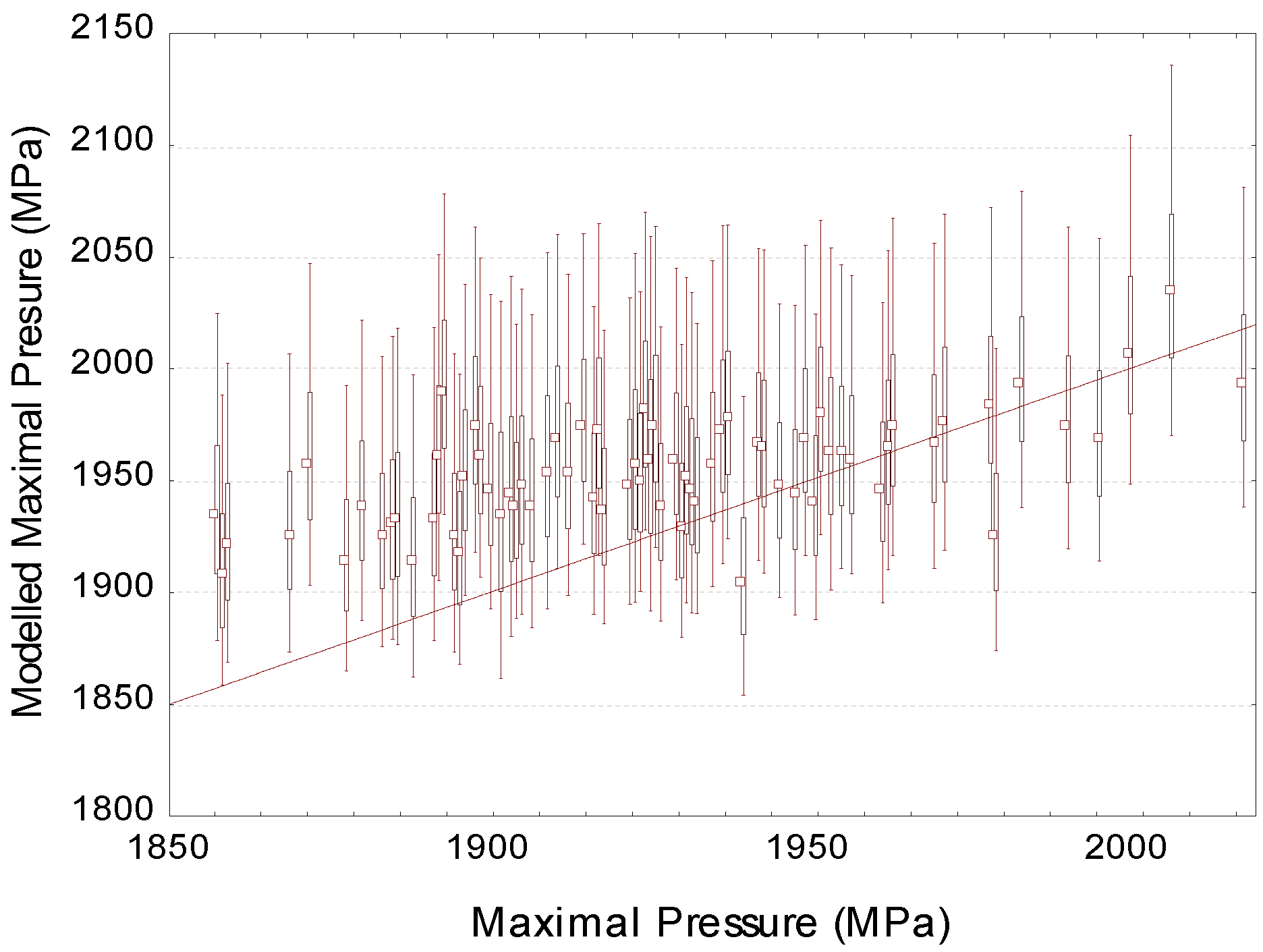
To validate the proposed protocols, one hundred surfaces are simulated and the experimental extreme values are extracted and compared to the PDF distributions of the maximal pressure. The Figure 7 represents the 90% confidence intervals of modeled data by the Lambda distribution versus the experimental values.
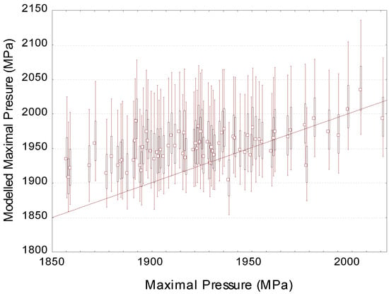
Figure 7.
The 90% confidence intervals of modeled data by the Lambda distribution for the maximal pressure versus the pressure data values. The straight line represents y = x.
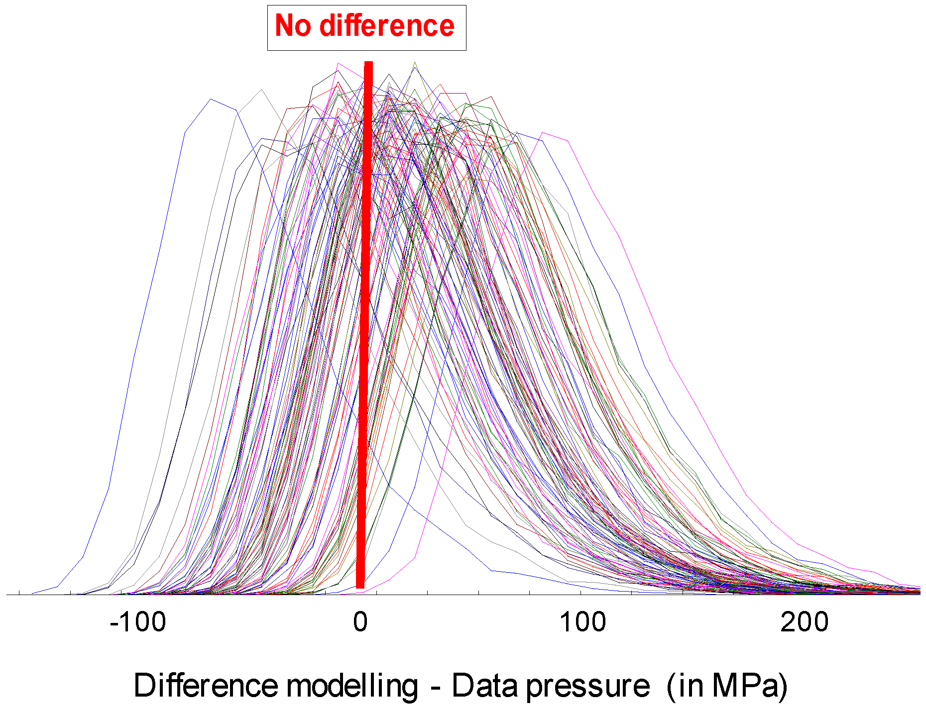
If the lambda distribution correctly fits the data, then the difference between the experimental data will be statistically equal to zero. To appreciate this hypothesis, the histograms of these differences are plotted for 100 surfaces (Figure 8). As is often the practice in statistics, the threshold of 95% is chosen to test the null value of the difference. Over all the one hundred surfaces, the null values is never rejected meaning that the lambda distribution describe correctly the extreme surface pressure.
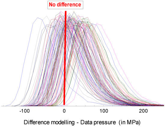
Figure 8.
The 90% confidence intervals of modeled data by the Lambda distribution for the maximal pressure versus the values predicted by the local contact model.
4. Experimental Validation
It is quite problematic to validate the proposed model experimentally. Indeed, the principle of our modeling of extreme pressure values is to look at the distribution of local pressures obtained from discretized mapping, then to search a polymorphic density model that then allows us to evaluate extreme pressure value. This extreme pressure value then gives a lower limit of the yield strength of the future material guaranteeing no plasticification on the investigated contact area. In our simulation, in order to stabilize the high variability of the probability density of pressures, 100 contact simulations are performed to determine a robust density of the GLD parameters of the contact pressures and its associated bootstrap estimators (see Figure 5). Numerically the convergence and robustness seem to be achieved with these 100 simulations on 100 different topographies. This clearly shows that it is necessary, in order to validate the proposed model, to perform 100 plane/contact surface indentation experiments, which will then give us a correct estimate of the maximum plastification stress. It should be noted that in the bibliography, many authors limit themselves to measuring only one surface to determine the average contact pressure, which cannot be enough to determine the maximum contact pressure. The experimental determination of extreme values will, therefore, require an automated process of plane/rough surface indentation. Indentations experiments will not directly estimate local contact pressure, but an average pressure and an estimate of the first contact of the peak of maximum amplitude and its spatial location. Beyond this metrological problem, another problem, often encountered in the bibliography proposing plane/rough surface indentation is the difficulty of morphologically quantifying whether a peak has plastified. Admittedly, if the surface has a fairly high percentage of plastified peaks, it becomes possible to estimate statistically the rate of plastification (Dowson reference), but it remains difficult to determine experimentally the peak that has the first plastified (flatness problem, elastic return, metrological errors of the topographic measurement…).
However, it is essential to validate the proposed methodology. In fact, our model is based on the probability of having the first peak that plastifies and to associate its contact pressure. The criticisms of our methodology that can be formulated are on the one hand, a simplistic model of contact simulation (justified by the large number of high-resolution simulations, discretization necessary to capture the morphology of the highest peaks) and on the other hand the difficulty of validating this methodology by a reasoned approach. To have a less critical modeling of the material’s behavior, finite element simulation seems tempting but remains complex at the level of elementary numerical operations. Even if this would prove possible in a reasonable time of calculations with the resolutions proposed in this article, it would prohibit us from future investigations on larger topographic resolutions (e.g., multi-fractal surfaces). Therefore, it is necessary to validate our approach without having to simulate our methodology by replacing our semi-analytical calculation with an MEF method. It is therefore necessary to build a methodology independent of the contact simulation method to validate the plasticification of extreme roughness and to associate them with a localized contact pressure without recourse to numerical calculation. For this purpose, we will have recourse to the nano-indentation test with of a Berkovich indentor. The nano-indenter continuously monitors the evolution of the tip depression with the indentation charge during the charging and discharging phases to observe the plastic and elastic response of the material. The tip used on our equipment is a Berkovich tip (pyramidal geometry with a triangular base). The indenter Berkovich is a three-sided pyramid, whose base is an equilateral triangle. The faces have an inclination of 65.3° with respect to the vertical axis. This homothetic geometry, therefore, makes it easy to identify the plasticized area by indentation. This homothetic geometry therefore makes it easy to identify morphologically the plastic area. A sample of the TA6V (MTS NanoIndentor) previously polished with 80 grade abrasive paper to obtain a rough surface is indented. Then the indentation print is recorded by atomic force microscopy (Bruker). Figure 9 (left) shows the topography where the angles of the indenter in plastic contact are visible. The non-indentated roughness has an Sa of 36 nm and the side of the impression in contact is equal to 18 µm.

Figure 9.
Nano-Indentation of TA6V samples (left), roughness extraction (center), indentation print measurements (right).
To carry out the simulation, we calculated the fractal dimension as well as the roughness (Sq), it was then possible to simulate a rough surface with the same property. Note that the summation of the function is limited in high frequencies to represent the beginning of the fractal regime of the roughness measured by AFM. Then the nano indentation test was simulated by an elasto-plastic model. Figure 10 shows the simulation of the indentation on the simulated rough surface (plastic zone is raised on the topographical map). The Sa of the simulated surface is closed to the experimental surface (Sa = 38 nm against Sa = 36 nm). This result shows that topographical simulation by the Weierstrass function leads to realistic rough surfaces. The elasto-plastic simulation shows a similar value on the indentation length 17 µm which validates our simulation model approach.

Figure 10.
Elasto-plastic simulation of TA6V material (left). To visualize the plastified area and frontier elastic/plastic deformations, the plastic area is raised through the elastic area. At the center, roughness extraction simulated by the 3D Weierstrass function and indentation print of simulated indentation print is shown on the right.
We will then postulate that at the elastoplastic transition boundary (see Figure 11 left) the pressure field is continuous due to the given shape between the surface and the indenter. This means that this boundary defines the transition zone and, therefore, the contact pressure is equal to the elastic limit of the materials. As a result, this boundary topography allows us to calculate the probability density function of asperities height at the beginning of plasticification. Figure 11 (center) represents this probability density function for the simulated and experimental plasticification frontiers for a given roughness height. As can be observed, the densities between the experimental and simulated measurement are quite close. It then becomes possible to determine the probability density of surface integrity (Figure 11, right). The experimental and simulated data are consistent, which validates the robustness of the simulation on a rough surface to detect local areas of first plastification.

Figure 11.
Frontier elastic/plastic deformations from elasto-plastic simulation of TA6V material (left). Probability density function of maximal roughness amplitude at plastification obtained from both simulated and experimental nano-indentations (center). Probability density function of surface integrity (right). 100% of integrity means that pass over a maximal peak amplitude of 0.43 µm, no plastification will occur).
5. Conclusions
In this paper, we proposed and exposed the principle of a statistical workflow to be applied to the analysis of rough surfaces in order to predict the statistics of contact pressure from roughness analysis. By means of the proposed functions, a statistical protocol allows us to extract the density of probability of the maximal pressure of a rough surface. This estimate is based upon a classical hypothesis of local elastic response of roughness peaks. The detailed validation of the proposed methodology could either involve contact pressure experimental measurements or numerical simulations taking into account the elastic interactions between peaks in future developments. The probability density of local contact pressure is described well by a GLD density function. Then, it is possible to determine the probability that the pressure of contact generates a plastic deformation from the analysis of the roughness statistics. The proposed methodology has been applied to numerically generated surfaces, but could also be adapted to the topography analysis of experimental ones. The influence of the sample size on this probability distribution variation can then be taken into account. From a statistical consideration, it should then become possible to plan the failure density of probability at a higher scale than the one use for scanning the sample. However, the uncertainties of measurements must be integrated to build a reliable probability density function of failure. The more experimental scanned surfaces, the better the prediction. Conversely, if the number of scanned surfaces is too weak, the elastic limit of the material must be increased to guarantee, with a fixed probability, the integrity of the structure, in order to get no damage of the structure by plastic deformation. The choice of the number of surfaces to be measured will become a compromise between the cost of the measure, the charge of the over-quality and the failure price. The workflow proposed in this paper, could contribute to finding the best traid-off and search for an optimal strategy in material elaboration.
Author Contributions
Conceptualization, Funding Acquisition, Writing and Formal Analysis, M.B.; Software, A.J.; validation, A.F.; investigation, F.P.; Nano Indentation and AFM measurements, F.R. All authors have read and agreed to the published version of the manuscript.
Funding
This research was funded by The ELSAT2020 project, co-financed by the European Union with the European Regional Development Fund, the French state and the Hauts de France Region.
Conflicts of Interest
The authors declare no conflict of interest.
Appendix A. The MultiScale Formulation of the Probability of Failure
The probability of failure will depends of the apparent surface area. If a one increases area, one increases the probability of having a higher pressure. If one suppose that the surface is ergodic, then double the surface area is equivalent to double the number of points of pressure in the pressure lambda PDF that stay unchanged according to ergodicity assumption. However, the extreme value PDF that depends on the number of sample points will change and becomes:
where k > 0 is the surface magnification factors, i.e., the predicted surfaces such where is the initial surface from which pressure PDF is evaluated.
Let the probability of surface integrities, then one computes by integration on the initial PDF that is and one finally get the multiscale PDF of surface integrities:
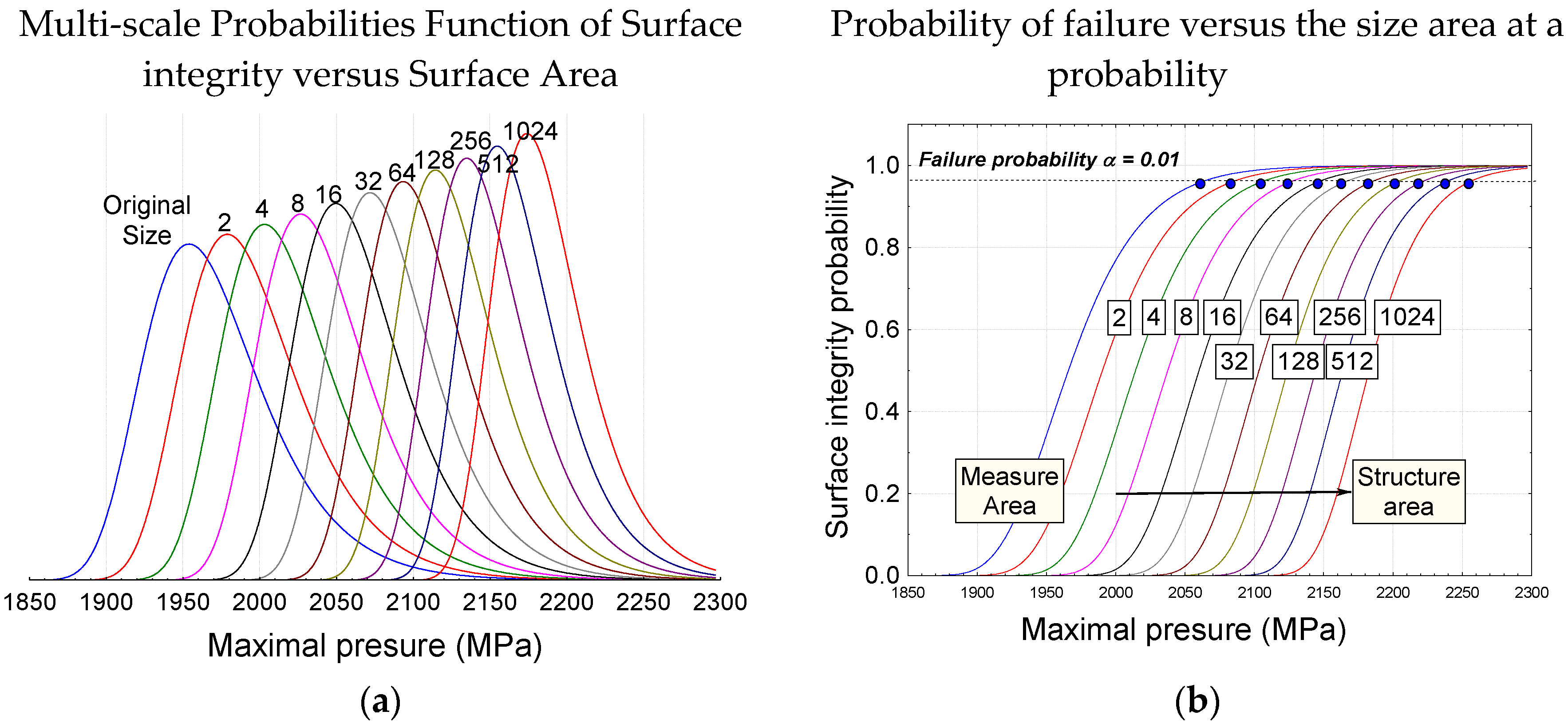
The Figure A1 (left) represents the multi-scale probabilities function of surface integrity versus surface area. This means that increasing the area of investigation compared to initial area increase the probability to find a higher maximal pressure. It becomes then possible to predict the maximal pressure assuring the integrity of a fixed area at a critical level α with only a measure on a lower surface area (Figure A1 right).
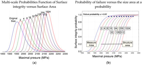
Figure A1.
(a) Multi-scale Probabilities Function of Surface integrity versus Surface Area; (b) Probability of failure versus the size area at a probability.
Figure A1.
(a) Multi-scale Probabilities Function of Surface integrity versus Surface Area; (b) Probability of failure versus the size area at a probability.
References
- Shen, J.; Liu, S.; Yi, K.; He, H.; Shao, J.; Fan, Z. Subsurface damage in optical substrates. Opt. Int. J. Light Electron Opt. 2005, 116, 288–294. [Google Scholar] [CrossRef]
- Fine, K.R.; Garbe, R.; Gip, T.; Nguyen, Q. Non-destructive, real time direct measurement of subsurface damage. In Proceedings of the SPIE, Orlando, FL, USA, 19 May 2005; Volume 5799, pp. 105–110. [Google Scholar]
- Stolz, C.J.; Menapace, J.A.; Schaffers, K.I.; Bibeau, C.; Thomas, M.D.; Griffin, A.J. Laser damage initiation and growth of antireflection coated S-FAP crystal surfaces prepared by pitch lap and magnetorheological finishing. In Proceedings of the SPIE, Boulder, CO, USA; 2005; Volume 5991, pp. 449–455. [Google Scholar]
- Campbell, J.H.; Hawley-Fedder, R.A.; Stolz, C.J.; Menapace, J.A.; Borden, M.R.; Whitman, P.K.; Yu, J.; Runkel, M.; Riley, M.O.; Feit, M.D.; et al. NIF optical materials and fabrication technologies: An overview. In Proceedings of the SPIE, San Jose, CA, USA, 28 May 2004; Volume 5341, pp. 84–101. [Google Scholar]
- Greenwood, J.A.; Williamson, J.P. Contact of nominally flat surfaces. In Proceedings of the Royal Society of London; Series A, Mathematical and Physical Sciences. Royal Society: London, UK, 1966; Volume 295, pp. 300–319. [Google Scholar]
- Greenwood, J.A.; Tripp, J.H. The contact of two nominally flat rough surfaces. Proc. Inst. Mech. Eng. 1970, 185, 625–633. [Google Scholar] [CrossRef]
- Tsukasa, T.; Anno, Y.; Fumio, K. Analysis of the deformation of contacting rough surface. Bull. JSME 1972, 15, 982–1003. [Google Scholar] [CrossRef]
- Van Zwol, P.J.; Svetovoy, V.B.; Palasantzas, G. Distance upon contact: Determination from roughness profile. Phys. Rev. B Condens. Matter Mater. Phys. 2009, 15, 996–1003. [Google Scholar] [CrossRef]
- Broer, W.; Palasantzas, G.; Knoester, J.; Svetovoy, V.B. Roughness correction to the Casimir force at short separations: Contact distance and extreme value statistics. Phys. Rev. B Condens. Matter Mater. Phys. 2012, 85, 155410. [Google Scholar] [CrossRef]
- Ponthus, N.; Scheibert, J.; Thøgersen, K.; Malthe-Sørenssen, A.; Perret-Liaudet, J. Statistics of the separation between sliding rigid rough surfaces: Simulations and extreme value theory approach. Phys. Rev. E 2019, 99, 023004. [Google Scholar] [CrossRef] [PubMed]
- Malekan, A.; Rouhani, S. Model of contact friction based on extreme value statistics. Friction 2019, 7, 327–339. [Google Scholar] [CrossRef]
- Bigerelle, M.; Najjar, D.; Iost, A. Multiscale functional analysis of wear: A fractal model of the grinding process. Wear 2005, 258, 232–239. [Google Scholar] [CrossRef][Green Version]
- Bhushan, B.; Majumdar, A. Elastic-plastic contact model for bifractal surfaces. Wear 1992, 153, 53–64. [Google Scholar] [CrossRef]
- Lopez, J.; Hansali, G.; Le Bossa, J.C.; Mathia, T. Caractérisation fractale de la rugosité tridimensionnelle d’une surface. J. Phys. III 1994, 4, 2501–2519. [Google Scholar] [CrossRef]
- Jourani, A.; Dursapt, M.; Hamdi, H.; Rech, J.; Zahouani, H. Effect of the belt grinding on the surface texture: Modeling of the contact and abrasive. Wear 2005, 259, 1137–1143. [Google Scholar] [CrossRef]
- Johnson, K.L. Contact Mechanics; Cambridge University Press: Cambridge, UK, 1985. [Google Scholar]
- Jourani, A.; Bigerelle, M.; Petit, L.; Zahouani, H. Local coefficient of friction, sub-surface stresses and temperature distribution during sliding contact. Int. J. Mater. Prod. Technol. 2010, 38, 44–56. [Google Scholar] [CrossRef]
- Jourani, A.; Hagege, B.; Bouvier, S.; Bigerelle, M.; Zahouani, H. Influence of abrasive grain geometry on friction coefficient and wear rate in belt finishing. Tribol. Int. 2013, 59, 30–37. [Google Scholar] [CrossRef]
- Gumbel, E.J. Statistical Theory of Extreme Values and Some Practical Applications; Applied Mathematics; National Bureau of Standards: Washington, DC, USA, 1954.
- Karian, Z.A.; Dudewicz, E.J. Fitting Statistical Distributions: The Generalized Lambda Distribution and Generalized Bootstrap Methods; Chapman & Hall: London, UK; CRC Press: Boca Raton, FL, USA, 2000. [Google Scholar]
- Karian, Z.A.; Dudewicz, E.J. Handbook of Fitting Statistical Distributions with R; Chapman & Hall: London, UK; CRC Press: Boca Raton, FL, USA, 2010. [Google Scholar]
- Najjar, D.; Bigerelle, M.; Lefebvre, C.; Iost, A. A new approach to predict the pit depth extreme value of a localized corrosion process. ISIJ Int. 2003, 43, 720–725. [Google Scholar] [CrossRef]
- Bigerelle, M.; Najjar, D.; Fournier, B.; Rupin, N.; Iost, A. Application of lambda distributions and bootstrap analysis to the prediction of fatigue lifetime and confidence intervals. Int. J. Fatigue 2006, 28, 223–236. [Google Scholar] [CrossRef][Green Version]
- Bigerelle, M.; Gautier, A.; Iost, A. Roughness characteristic length scales of micro-machined surfaces: A multi-scale modeling. Sens. Actuators B Chem. 2007, 126, 126–137. [Google Scholar] [CrossRef]
- Fournier, B.; Rupin, N.; Bigerelle, M.; Najjar, D.; Iost, A.; Wilcox, R. Estimating the parameters of a generalized lambda distribution. Comput. Stat. Data Anal. 2007, 51, 2813–2835. [Google Scholar] [CrossRef]
- Fournier, B.; Rupin, N.; Bigerelle, M.; Najjar, D.; Iost, A. Application of the generalized lambda distributions in a statistical process control methodology. J. Process Control 2006, 16, 1087–1098. [Google Scholar] [CrossRef]
- Efron, B. Bootstrap methods: Another look at the Jackknife. Ann. Stat. 1979, 7, 1–26. [Google Scholar] [CrossRef]
- Efron, B.; Tibshirani, R. An Introduction to the Bootstrap; Chapman & Hall: New York, NY, USA, 1993. [Google Scholar]
- Bowden, F.P.; Tabor, D. The Friction and Lubrication of Solids; Oxford University Press: Oxford, UK, 2001. [Google Scholar]
© 2019 by the authors. Licensee MDPI, Basel, Switzerland. This article is an open access article distributed under the terms and conditions of the Creative Commons Attribution (CC BY) license (http://creativecommons.org/licenses/by/4.0/).


