Sensitivity Analysis of Rotor/Stator Interactions Accounting for Wear and Thermal Effects within Low- and High-Pressure Compressor Stages

Abstract
:1. Introduction
2. Numerical Model
2.1. Blade
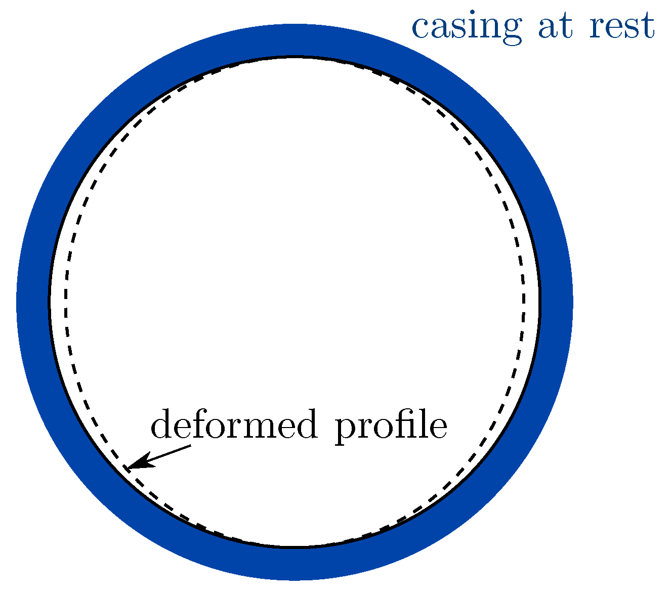
2.2. Casing
2.3. Abradable Coating
2.3.1. Mechanical Mesh
2.3.2. Thermal Mesh
2.3.3. Thermo-Mechanical Coupling
2.4. Summary
3. Convergence Analysis
4. Experiments
4.1. Calibration of the Thermal Model
4.2. Application of the Calibrated Model
4.3. Partial Conclusion
5. Sensitivity Analysis
5.1. High-Pressure Compressor Blade
5.1.1. Influence of the Angular Speed
5.1.2. Influence of the Initial Clearance
5.1.3. Cross Analysis
 ) at higher angular speed for low initial gap values, 17 wear lobes (
  ) at low initial gap values, and 22 wear lobes (
  ) for intermediate gap values.
5.2. Low-Pressure Compressor Blade
5.2.1. Influence of the Angular Speed
5.2.2. Influence of the Initial Clearance
5.2.3. Cross Analysis
), and 15 wear lobes ( ). As for the HP compressor blade, the higher the angular speed, the lower initial clearance interactions occur. However, the two interaction areas are here well separated, with a more stable initiation of the interaction with the initial conditions. The 15 wear lobes is observed only at lower angular speed while the 7th engine order interaction responds for a large range of angular speeds and initial clearances. This cross analysis shows that depending on the engine nominal angular speed, a reduction of the nominal clearances in the engine design in order to improve the aerodynamic performance can lead to a risk of occurrence of interactions with other engine orders.6. Conclusions
Author Contributions
Funding
Conflicts of Interest
References
- Williams, R.J. Simulation of blade casing interaction phenomena in gas turbines resulting from heavy tip rubs using an implicit time marching method. In Proceedings of the ASME Turbo Expo 2011 Conference, GT2011-45495, Vancouver, BC, Canada, 6–11 June 2011. [Google Scholar]
- Millecamps, A.; Brunel, J.; Dufrénoy, P.; Garcin, F.; Nucci, M. Influence of thermal effects during blade-casing contact experiments. In Proceedings of the ASME 2009 IDETC & CIE Conference, ASME, San Diego, CA, USA, 30 August–2 September 2009. [Google Scholar]
- Batailly, A.; Agrapart, Q.; Millecamps, A.; Brunel, J.F. Experimental and numerical simulation of a rotor/stator interaction event within an industrial high-pressure compressor. J. Sound Vib. 2016, 375, 308–331. [Google Scholar] [CrossRef] [Green Version]
- Muszynska, A.; Bently, D.; Franklin, W.; Hayashida, R.; Kingsley, L.; Curry, A. Influence of Rubbing on Rotor Dynamics—Part 1; Technical Report NAS8-36179; NASA: Washington, DC, USA, 1989. [Google Scholar]
- Borel, M.; Nicoll, A.; Schlapfer, H.; Schmid, R. The wear mechanisms occurring in abradable seals of gas turbines. Surf. Coat. Technol. 1989, 39, 117–126. [Google Scholar] [CrossRef] [Green Version]
- Mandard, R.; Witz, J.F.; Boidin, X.; Fabis, J.; Desplanques, Y.; Meriaux, J. Interacting force estimation during blade/seal rubs. Tribol. Int. 2015, 82, 504–513. [Google Scholar] [CrossRef] [Green Version]
- Salles, L.; Blanc, L.; Thouverez, F.; Gouskov, A. Dynamic analysis of fretting wear in friction contact interfaces. Int. J. Solids Struct. 2010, 48, 1513–1524. [Google Scholar] [CrossRef] [Green Version]
- Baïz, S. Etude expérimentale du contact aube/abradable: contribution à la caractérisation mécanique des matériaux abradables et de leur interaction dynamique sur banc rotatif avec une aube. Ph.D. Thesis, Ecole Centrale de Lille, Villeneuve-d’Ascq, France, 2011. [Google Scholar]
- Legrand, M.; Batailly, A.; Pierre, C. Numerical investigation of abradable coating removal through plastic constitutive law in aircraft engine. J. Comput. Nonlinear Dyn. 2011, 7, 011010. [Google Scholar] [CrossRef]
- Nyssen, F.; Batailly, A. Thermo-Mechanical Modeling of Abradable Coating Wear in Aircraft Engines. J. Eng. Gas Turbines Power 2019, 141, 021031. [Google Scholar] [CrossRef] [Green Version]
- Sternchüss, A.; Balmès, E. On the reduction of quasi-cyclic disks with variable rotation speeds. In Proceedings of the International Conference on Advanced Acoustics and Vibration Engineering (ISMA), Leuven, Belgium, 18–20 September 2006; pp. 3925–3939. [Google Scholar]
- Palfrey-Sneddon, H.; Neely, A.J.; Smith, E.O. The influence of descent and taxi profiles on the thermal state of a jet engine at shutdown. In Proceedings of the ISABE 2017 Conference, Manchester, UK, 3–8 September 2017. [Google Scholar]
- Adam, L. Modélisation du comportement thermo-élasto-viscoplastique des métaux soumis à grandes déformations. Application au formage superplastique. Ph.D. Thesis, Université de Liège, Liège, Belgium, 2003. [Google Scholar]
- Debard, Y. Méthode des éléments finis: thermique; Université du Mans: Le Mans, France, 2011. [Google Scholar]
- Jeong, C.Y. Effect of Alloying Elements on High TemperatureMechanical Properties for Piston Alloy. Mater. Trans. 2012, 53, 234–239. [Google Scholar] [CrossRef] [Green Version]
- Batailly, A.; Legrand, M.; Millecamps, A.; Garcin, F. Conjectural bifurcation analysis of the contact-induced vibratory response of an aircraft engine blade. J. Sound Vib. 2015, 348, 239–262. [Google Scholar] [CrossRef] [Green Version]
- Layachi, M.Y.; Bölcs, A. Effect of the axial spacing between rotor and stator with regard to the indexing in an axial compressor. In Proceedings of the ASME Turbo Expo 2001 Conference, GT2017-64342, New Orleans, LA, USA, 4–8 June 2001. [Google Scholar]
- Ameli, A. Numerical simulation of rotor/stator interaction and tip clearance flow in centrifugal compressors. Master’s Thesis, Lappeenranta University of Technology, Lappeenranta, Finland, 2015. [Google Scholar]
- Gourdain, N.; Wiassow, F.; Ottavy, X. Effect of Tip Clearance Dimensions and Control of Unsteady Flows in a Multi-Stage High-Pressure Compressor. J. Turbomach. 2012, 134, 051005. [Google Scholar] [CrossRef]
- Feng, J.; Luo, X.; Guo, P.; Wu, G. Influence of tip clearance on pressure fluctuations in an axial flow pump. J. Mech. Sci. Technol. 2016, 30, 1603–1610. [Google Scholar] [CrossRef]


 /
/  ), or ( / ), or (
  /
/  ), or (
  /
/  ).
/ ), or ( / ), or ( / ), or ( / ).
).
/ ), or ( / ), or ( / ), or ( / ).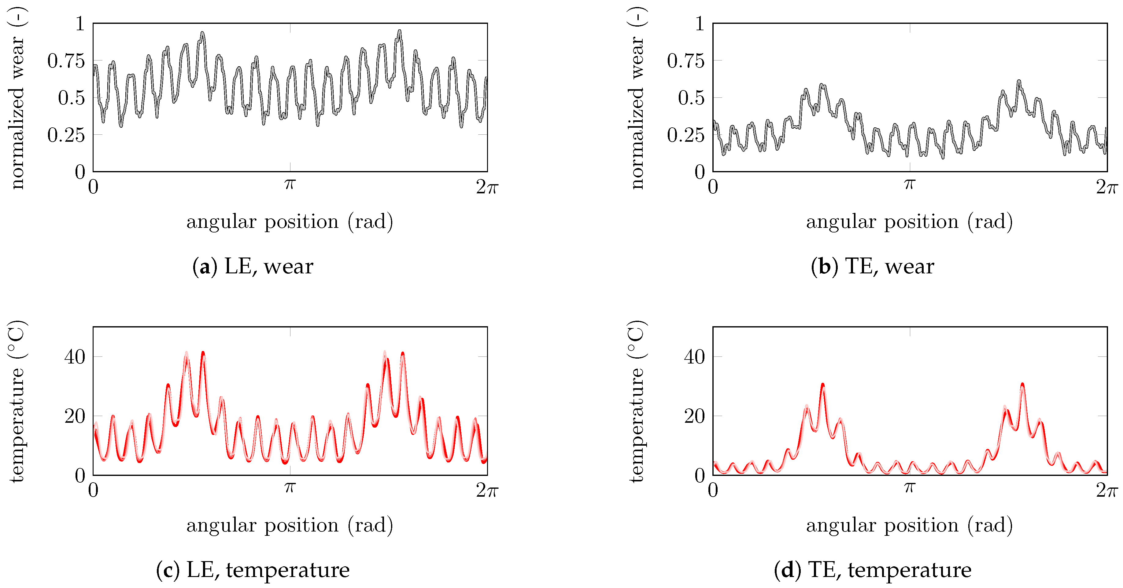 / ), ( / ), ( / ), ( / ).
/ ), ( / ), ( / ), ( / ).
/ ), ( / ), ( / ), ( / ).
 ), (
), (  ), (
), (  ), (
), (  ), and (b) : ( ), ( ), ( ), ( ).
), ( ), ( ), ( ), and (b) : ( ), ( ), ( ), ( ).
), and (b) : ( ), ( ), ( ), ( ).
), ( ), ( ), ( ), and (b) : ( ), ( ), ( ), ( ).


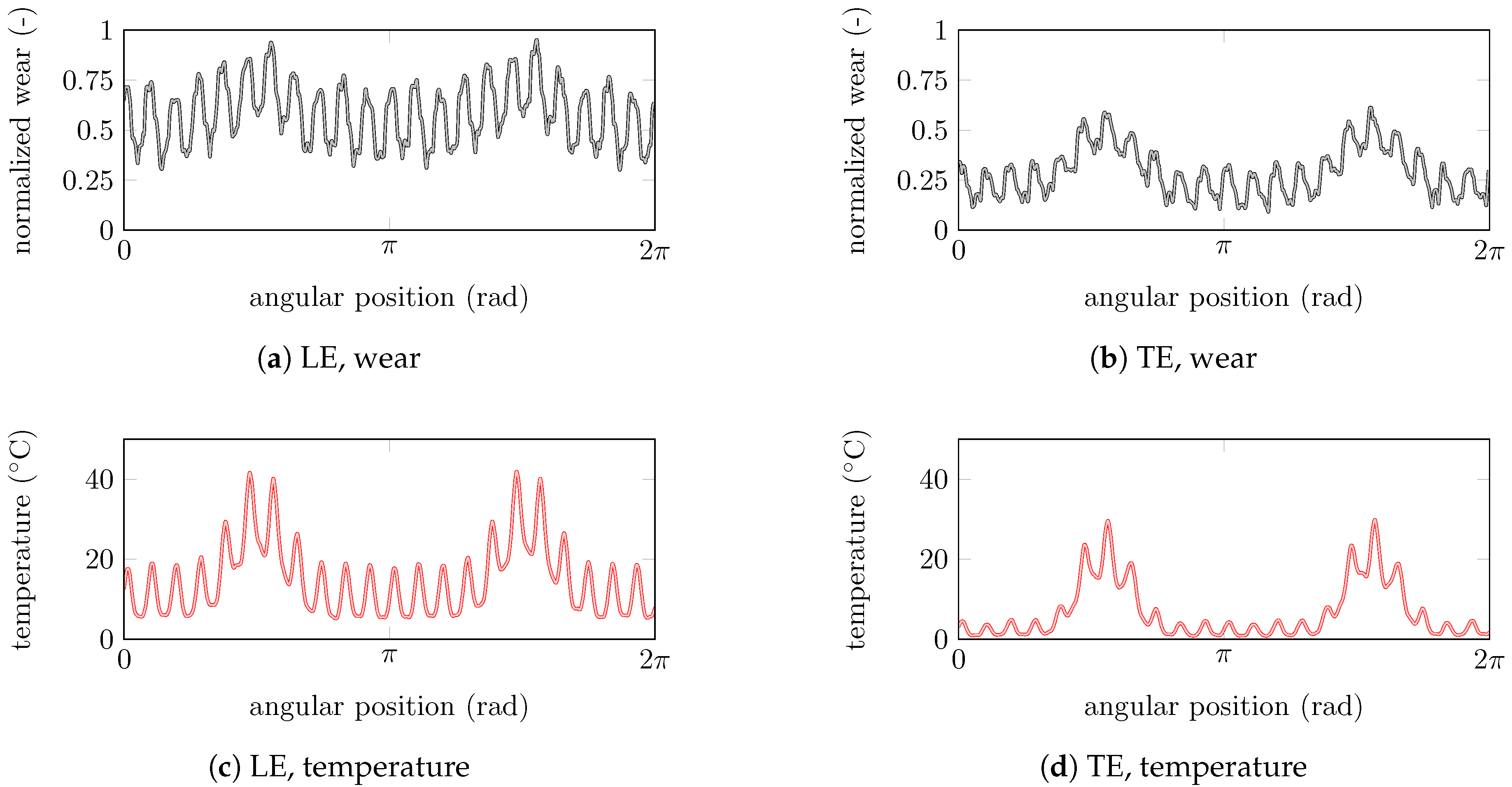
 ), mid-chord ( ), and trailing edge ( ) for the HP compressor test case.
), mid-chord ( ), and trailing edge ( ) for the HP compressor test case.
), mid-chord ( ), and trailing edge ( ) for the HP compressor test case.


 ), mid-chord ( ), and trailing edge ( ) for the LP compressor test case.
), mid-chord ( ), and trailing edge ( ) for the LP compressor test case.
), mid-chord ( ), and trailing edge ( ) for the LP compressor test case.


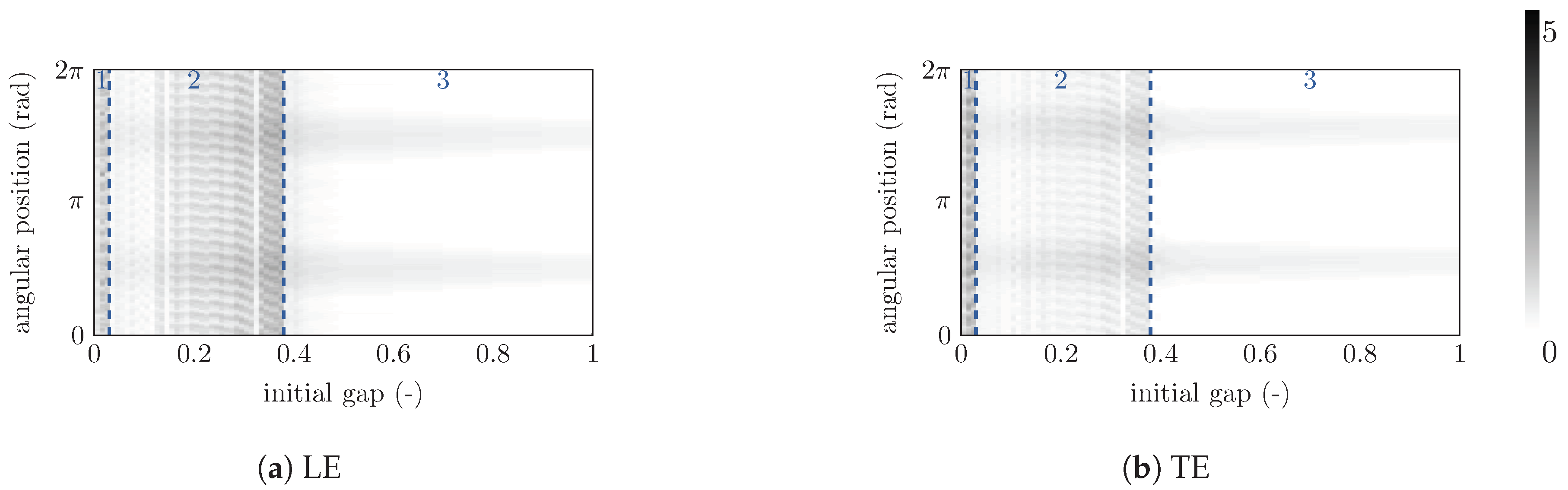

 ): 5 wear lobes, ( ): 17 wear lobes, ( ): 22 wear lobes.
): 5 wear lobes, ( ): 17 wear lobes, ( ): 22 wear lobes.
): 5 wear lobes, ( ): 17 wear lobes, ( ): 22 wear lobes.


 ): 7 wear lobes, ( ): 15 wear lobes.
): 7 wear lobes, ( ): 15 wear lobes.
): 7 wear lobes, ( ): 15 wear lobes.
© 2020 by the authors. Licensee MDPI, Basel, Switzerland. This article is an open access article distributed under the terms and conditions of the Creative Commons Attribution (CC BY) license (http://creativecommons.org/licenses/by/4.0/).
Share and Cite
Nyssen, F.; Batailly, A. Sensitivity Analysis of Rotor/Stator Interactions Accounting for Wear and Thermal Effects within Low- and High-Pressure Compressor Stages. Coatings 2020, 10, 74. https://doi.org/10.3390/coatings10010074
Nyssen F, Batailly A. Sensitivity Analysis of Rotor/Stator Interactions Accounting for Wear and Thermal Effects within Low- and High-Pressure Compressor Stages. Coatings. 2020; 10(1):74. https://doi.org/10.3390/coatings10010074
Chicago/Turabian StyleNyssen, Florence, and Alain Batailly. 2020. "Sensitivity Analysis of Rotor/Stator Interactions Accounting for Wear and Thermal Effects within Low- and High-Pressure Compressor Stages" Coatings 10, no. 1: 74. https://doi.org/10.3390/coatings10010074