Abstract
This article describes the development of a mathematical model of the reverse roll coating of a thin film for an incompressible non-isothermal magnetohydrodynamics viscoplastic fluid as it passes through a small gap between two rolls rotating reversely. The equations of motion required for the fluid added to the web are constructed and simplified using the lubrication approximation theory . Analytical results are obtained for the velocity profile, pressure gradient, and temperature distribution. The pressure distributions and flow rate are calculated numerically using the trapezoidal rule and regular false position method, respectively. Some of these results are presented graphically, while others are shown in a tabular form. From the present analysis, it has been observed that the magnitude of pressure distributions increases by increasing the value of the involved parameters. It is worth mentioning that the velocities ratio and Brickman’s number are controlling parameters for the temperature distributions. The results indicate the strong effectiveness of the viscoplastic parameter and velocities ratio for the velocity and pressure distributions. It is also concluded that the coating of Casson material has been remarkably affected by the magnetohydrodynamics effects.
1. Introduction
The coating of surfaces with a liquid film is frequently used in the magnetic tape, photography, and wrapper industries and for paint and paper to shield a sizeable surface region with one/numerous uniform layers. Even though the products used in these coating industries vary widely, the same fundamental technologies are considered to manufacture the needed coatings and films. A wide range of procedures are available to attain the goal of a fluid layer on a surface continuously. The choice of the scheme, however, hinges on numerous factors—for example, the liquid rheology, the nature of the surface being covered, the dry thickness to be required, the solvent used, the uniformity of the cover, the speed of the covering technique, etc. [1,2,3].
Generally, a liquid film should be uniform in thickness, continuous, and thin. Under certain operating conditions, of course, instabilities in films are observed, which can only be explored by deliberating the problems of fluid dynamics related to the coating process, as a nonlinear occurrence is seen in the procedure [4,5] for Newtonian flows. Chandio and Webster [6] developed a numerical scheme purely based on the methodology of finite elements with the prediction of a free surface in time and presented an analysis of transient instabilities with a variable speed ratio. It was observed that flow instabilities increase with an increase in the speed of the foil rather than with the speed of the roll. Industrially, at high line speeds a main disadvantage is underlined by the occurrence of flow instabilities, causing flaws that yield the form of the “ribbing” of the exerted coating (3D effects).
The roll coating process is most widely employed in industry because of its consistency in the implementation of fluids through revolving rolls [7]—for example, in the implementation of functioning organic coatings to steel strips, in structural laminating applications, and in the utilization of water-based adhesives to tapes. One side of the substrate (strip, sheet) is covered with a fluid layer as it goes through rotating cylindrical rollers on the opposite side (reverse roll mode) [8,9]. A significant component of roller coating is the existence of a static space between the rollers; such a flow of a fluid in the space is the main factor controlling the thickness and consistency of the coated film. In the nip between the rotating rollers, the fluid undergoes high deformation rates over a very short period [10].
Roll coating, as a process, is extremely versatile but involves technical and operational skills to maintain consistency. The application of a covered steel strip in the manufacture industry nowadays is expanding to more innovative functions such as coatings that afford acoustic protection or photovoltaic coatings used to collect solar energy. There is also a continuous struggle to increase coating line speeds because of economic issues, while taking care of the demand to control the weight of the film and the absence of defects [8,9,10,11].
In the process of roll coating, the gap among the two rotating rolls is considerably shorter than the radii of the rollers and is generally divided into three categories—namely, reverse roll coating (RRC), metering roll coating, and forward roll coating. In the case of forward roll coating, the two rolls at the nip go in alike directions. The coating fluid forms a bath on the nip’s upstream side and, after leaving the nip, divides into two liquid films which are transformed on both sides of the roller; one of them is applied for industrial purposes to a web. The rollers move in the opposite direction, with the reverse roller coating and the metering coating on the nip. The flow of leakage through the nip is reprocessed and the transported flow is deposited to the sheet for reverse rolling. The leakage flux flow on the sheet creates a uniform metered film while the roll coating is metering. It can be realized that the flow field configurations between two rotating rollers are alike for these two coating methods. Therefore, both are commonly referred to as reverse roll coating systems [12,13,14,15,16].
The flow problems of the roll coating methods have been studied in detail in recent decades, including in experimental work, theoretical approaches, and numerical analyses. The forward roll coating was of fundamental importance among these, and was the most commonly addressed. Experimental research on this has been performed by Benkreira et al. [17], Greener and Middleman et al. [18], and Decrees et al. [19], while theoretical analyses have been presented by Benkreira et al. [20] and Greener and Middleman et al. [18]. Reverse roll coating studies have received far less consideration as compared to forward roll coating [21].
The lubrication theory has been employed in previous works by Greener and Middleman et al. [22] and Holland et al. [23] for the simplification of equations of motion to study reverse roll coating systems; however, no attention has been paid to analyzing the effects of surface tension, the existence of free surfaces, and fluid contact lines. Coyle et al. [24] developed a finite element approach which was followed by experimental outcomes to express the fundamental fluid dynamics properties of reverse roll coating. They also illustrated the existence of flow instabilities, including ribbing and cascading. Hao et al. [12] established the Galeriken finite element technique to evaluate the coating flow among two rotating reverse rolls. Using the lubrication theory, Taylor and Zettlemoyer [25] observed the ink flow behavior in the process of printing presses. They obtained the effects of pressure distribution and force. The water flow between two rolls was discussed by Hinter Maier and White [26]. They used the principle of lubrication and presented findings that were consistent with their experimental results. Belblidia et al. [8] developed a flawless model of reverse roll coating using the algorithm of Taylor and Galerkin for pressure correction at high speed. The innovation of the work is encouraged by the need in coating manufacturing to coat stably, faster, and with uniform thin layers by optimizing the coater operating conditions and coating rheology. Zahid et al. [27] have debated the roll-coating analysis of an incompressible viscoelastic liquid when both roll and sheet have uniform speeds. The simplified form of the equation of motion was obtained by utilizing the lubrication approximation theory. Analytical expressions of the velocity profile, flow rate per unit width, pressure gradient, and shear stress were demonstrated on the roll surface. Recently, Zahid et al. [28] studied second-grade materials and explored engineering parameters of interest, such as pressure distribution, strength, coating thickness, split location, stress, roller power input, and adiabatic temperature rise.
To the best of our understanding, there is no reference to the theoretical formulation of the reverse roll coating with the Casson fluid model. The aim of the present work is to develop a mathematical model for the flow mechanism of viscoplastic fluid roller coating in the presence of magnetohydrodynamics and to analyze this theoretically.
2. The Problem Formulation and Governing Equations
Consider a laminar, steady, non-isothermal, MHD flow of an incompressible viscoplastic fluid between two heated rolls rotating in the opposite direction with velocities and , where is the radius of each roll and the subscripts and stand for forward and reverse rotating rolls, respectively. The minimum distance between two rotating rollers is called the nip region, and the distance at the nip region is presented by . Furthermore, the is taken along the flow movement, while the is considered transverse to the direction of the flow, as presented in Figure 1.
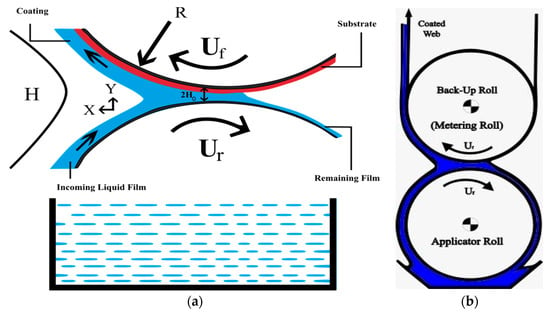
Figure 1.
(a) Schematic representation of the reverse roll coating process, (b) reverse roll operation.
The Casson fluid model’s motion is debated through the following equations for the conservation of mass and momentum:
where represents the velocity filed; is the density; is the specific heat capacity; is the pressure; represents the current density; is the time; represents the total magnetic field with , where and represent the applied and induced magnetic field, respectively; is the thermal conductivity; is the temperature; represents the gradient of the velocity; and the extra stress tensor is represented by for the Casson fluid model. The rheological equation of the extra stress tensor for the isotropic and incompressible flow of the Casson fluid may be given as [29]:
where is the yield stress, represents the viscosity of plastic properties for non-Newtonian fluids, represents the product of the component deformation rate with itself and based on the model of non-Newtonian fluid, and the term is the critical value of this product.
For two-dimensional flow, we take:
In Equation (5) and are the velocity components in direction and direction, respectively, and:
We assume the electric field to be zero and the induced magnetic field to be very small compared with the applied magnetic field, so that the magnetic Reynolds number is negligible [30]. Then, the Lorentz force given by becomes (where represents the electric conductivity of the fluid), so that the applied magnetic field only contributes to the electrical density. In this case, due to the magnetic field the Lorentz force becomes:
With the help of Equations (1), (4) and (5), Equations (2) and (3) may be written as:
where and are termed as the normal stresses and .
2.1. Lubrication Approximation Theory Analysis
From the problem’s geometry, we account that the most significant dynamic phenomenon occurs in the reverse roll coating at the nip. The minimal gap at the nip region is presented by between rolls. Thus, it may be useful to assume that there are almost parallel flows, such that the common fluid motion is mostly in the direction, while the minimal velocity of the fluid is in the direction. Furthermore, the change in velocity in the direction is dominant over the change in velocity in the direction. To simplify, we can perform an order of magnitude analysis to find the scale of pressure and velocity characteristics, so that we can identify , , and as , , and . Taking into account these relations and in view of the equation of continuity, we have , where . This debate leads us to write Equations (8) and (9) as:
From Equation (12), it is clear that is the function of —i.e., —therefore Equations (11)–(13) reduce to:
where represents the viscoplastic Casson parameter.
2.2. The Dimensionless Equations
The dimensionless parameters are defined as:
Then, the dimensionless forms of Equations (14) and (15) become:
where , , and and and are Eckert and Prandtl numbers and represents the Brinkman number , respectively.
The dimensionless boundary conditions subject to Equations (17) and (18) become:
where is velocity ratio of the reverse roll to forward roll.
2.3. The Solution to the Problem
The solution of Equation (17) using the boundary conditions given in Equation (19) becomes:
The dimensionless flow rate through the nip is defined as:
The pressure gradient from Equation (22) becomes:
The analytical solution of Equation (23) is difficult to obtain. Thus, we have been applied the numerical technique called the trapezoidal rule with the boundary condition as to obtain an expression for the pressure.
A simple second material balance relationship for is defined as:
where and are the velocities of reverse and forward roll, respectively. Equation (24) may be led to the expression given by:
where is the coating thickness, , where is half of the nip separation gap between the two rolls and and are the thickness of the fluid film on the reverse and forward roll, respectively. Thus, to determine the thickness of the coating and the pressure distribution, we need to find the value of . To determine the equation, we impose the Swift–Stieber boundary conditions on the pressure. It is claimed that at the transition point , both the pressure and pressure gradient disappear, and the lubrication type flow turns into a transverse. Upon setting , we get:
We integrate Equation (23) to obtain the value of pressure distribution. In view of the Swift–Stieber boundary condition for pressure, replacing with everywhere in the resulting equation of pressure and then setting into it the value of in terms of from Equation (26), the transcendental equation in is obtained. Using a numerical method—namely, the regular false position method—we obtain results for , which are shown in Table 1, Table 2 and Table 3.

Table 1.
Effect of by fixing , , .
Table 2.
Effect of by fixing , , .
Table 3.
Effect of by fixing , , .
2.4. The Solution of Temperature
Now using the velocity distribution Equation (20) in Equation (18), we get:
where is defined in Equation (23). Solving Equation (27) subject to the boundary conditions given in Equation (19), we get:
where:
and
2.5. Operating Variables
The desired engineering parameters of interest can be easily determined once the velocity, pressure distribution, and pressure gradient have been calculated.
2.5.1. Separating Force
The separating force of the rolls is as follows:
where represents the roll-separating force per unit width in dimensional form.
2.5.2. Power Input
The integral given below calculates the power delivered to the fluid by the roll.
Here, is the dimensionless power and the dimensionless share stress component is defined as .
2.5.3. Nusselt Number
The (Nusselt number) at the upper roll surface is defined as:
Using Equation (28), we get:
Similarly,
3. Results and Discussion
This article analyzes the reverse roll coating process for an incompressible non-isothermal viscoplastic material. By using the lubrication approximation theory, the flow equations are simplified. Closed-form solutions for the velocity profile, flow rate, pressure gradient temperature distribution, separating force, power input, and Nusselt numbers are obtained. Since the equation of pressure gradient is a complex equation, its exact solution is impossible. Therefore, we used the trapezoidal rule to find the numeric expression for pressure with a predefined tolerance . Further, in order to find the flow rate, the regular false position method is employed. The computational time of the numerical method for the simulation depends upon the desired accuracy and step-size taken in this regard. It means that the higher the accuracy desired, the greater the computational time.
Table 1, Table 2, Table 3 and Table 4 give the numerical results of the flow characteristics, such as flow rate, separation/transition points, coating thickness, separation force, and power input for different values of parameters in the domain. The typical velocity profiles have been illustrated in Figure 2, Figure 3, Figure 4, Figure 5, Figure 6, Figure 7, Figure 8, Figure 9 and Figure 10 at various positions of the channel of the roll coating process through variation in the velocities ratio , the MHD parameter , and the viscoelastic parameter . The graphical representations of the pressure gradient and pressure distributions have been sketched in Figure 11, Figure 12, Figure 13, Figure 14, Figure 15 and Figure 16. Figure 17, Figure 18, Figure 19, Figure 20, Figure 21, Figure 22, Figure 23, Figure 24, Figure 25, Figure 26, Figure 27 and Figure 28 present the variation in the temperature distribution in the given domain, whereas the relation between the velocities ratio of the rolls and the coating thickness can be seen in Figure 29 and Figure 30.
Table 4.
Effect of on the coating thickness.
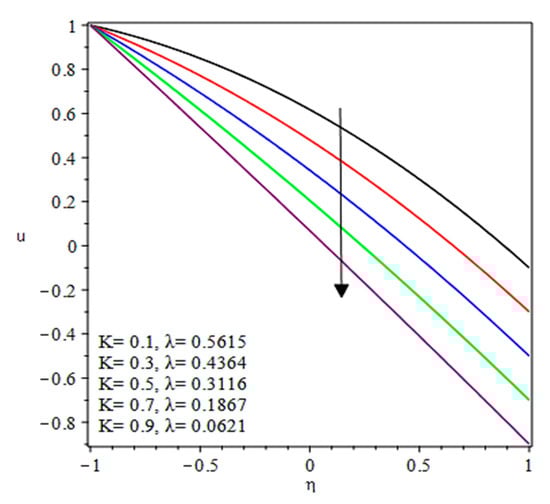
Figure 2.
Influence of on the velocity profile at by fixing and .
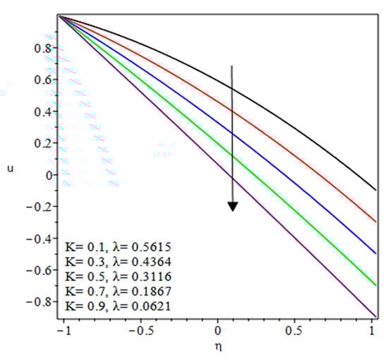
Figure 3.
Influence of on the velocity profile at by fixing and .
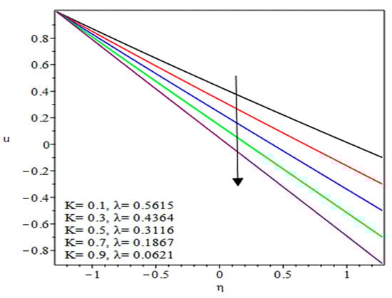
Figure 4.
Influence of on the velocity profile at by fixing and .
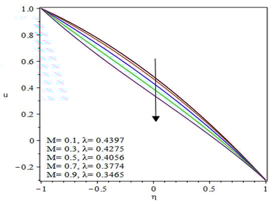
Figure 5.
MHD parameter influence on the velocity profile at by fixing and .
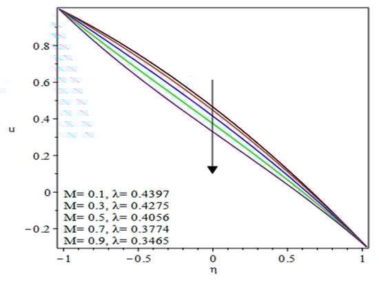
Figure 6.
MHD parameter influence on the velocity profile at by fixing and .
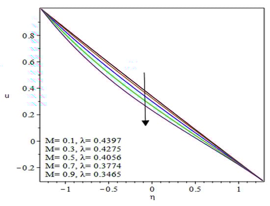
Figure 7.
MHD parameter influence on the velocity profile at by fixing and .
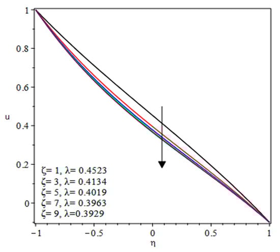
Figure 8.
Viscoplastic parameter influence on the velocity profile at by fixing , .
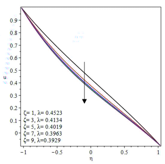
Figure 9.
Viscoplastic parameter influence on the velocity profile at by fixing , .
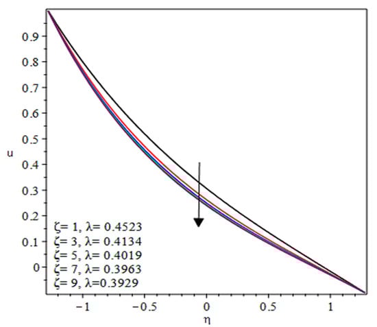
Figure 10.
Viscoplastic parameter influence on the velocity profile at by fixing , .
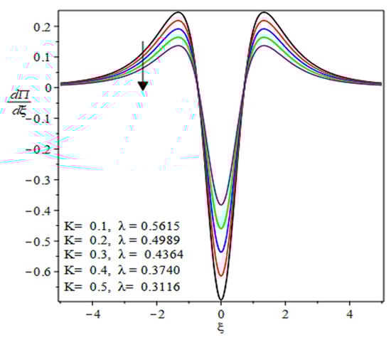
Figure 11.
Influence of on the pressure gradient by fixing , .
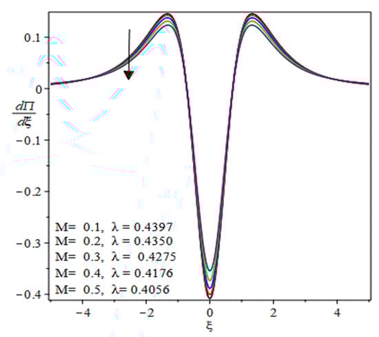
Figure 12.
MHD parameter influence on the pressure gradient by fixing , .
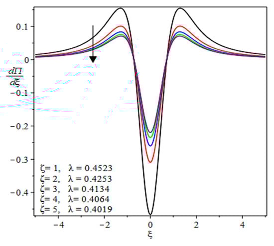
Figure 13.
Viscoelastic parameter influence on the pressure gradient by fixing , .
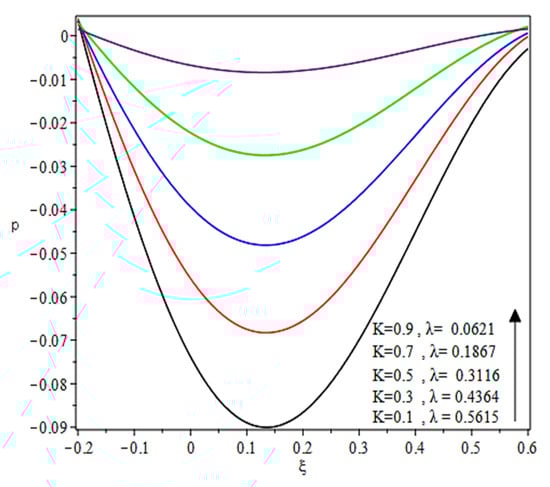
Figure 14.
Influence of on the pressure distribution by fixing , .
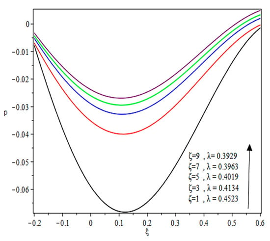
Figure 15.
Viscoelastic parameter influence on the pressure distribution by fixing , .
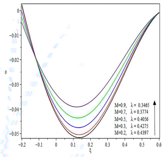
Figure 16.
MHD influence on the pressure distribution by fixing , .
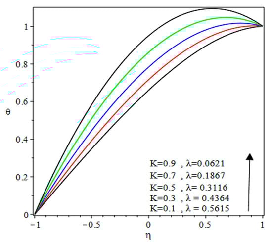
Figure 17.
Influence of on the temperature distribution at .
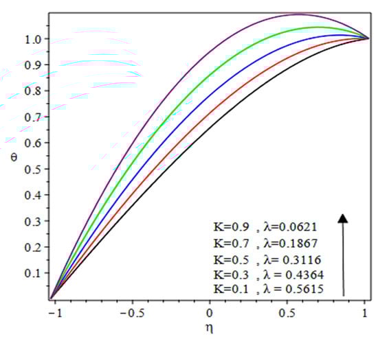
Figure 18.
Influence of on the temperature distribution at .
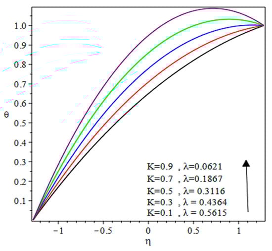
Figure 19.
Influence of on the temperature distribution at .
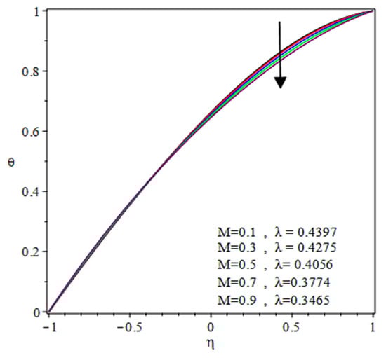
Figure 20.
Influence of on the temperature distribution at .
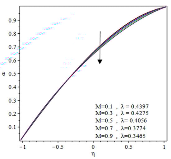
Figure 21.
Influence of on the temperature distribution at .
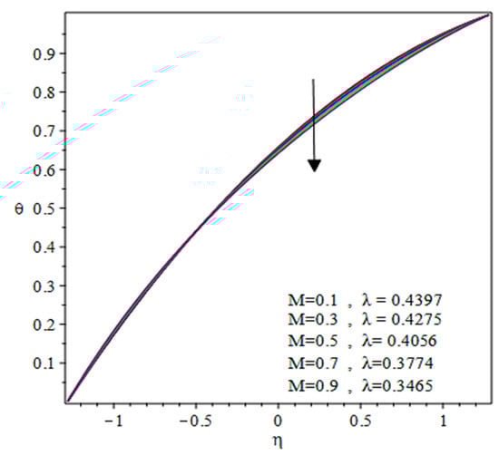
Figure 22.
Influence of on the temperature distribution at .
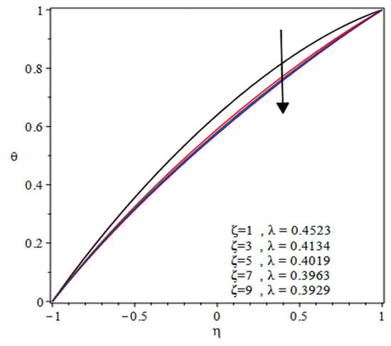
Figure 23.
Viscoplastic parameter influence on the temperature distribution at .
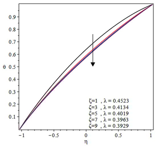
Figure 24.
Viscoplastic parameter influence on the temperature distribution at .
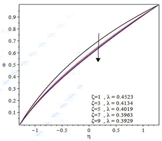
Figure 25.
Viscoplastic parameter influence on the temperature distribution at .
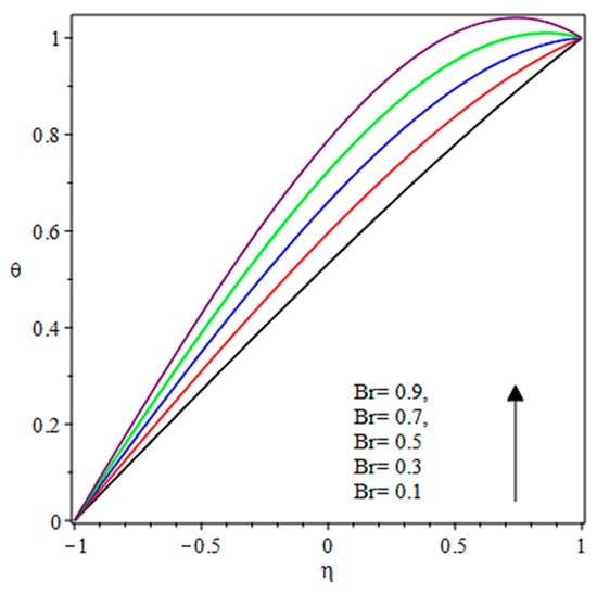
Figure 26.
Influence of on the temperate distribution at .
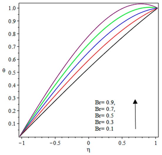
Figure 27.
Influence of on the temperate distribution at .
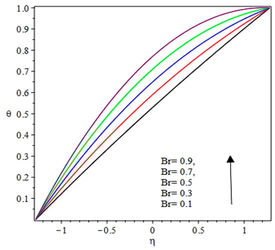
Figure 28.
Influence of on the temperate distribution at .
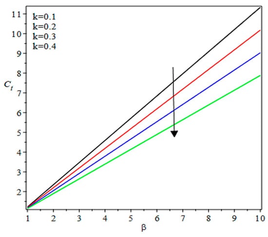
Figure 29.
Influence of the velocities ratio on the coating thickness.
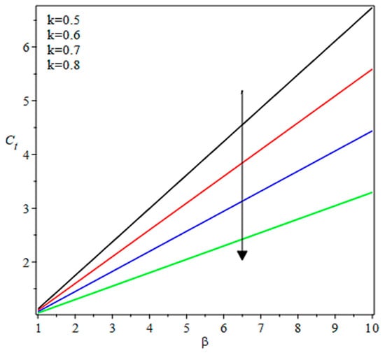
Figure 30.
Influence of the velocities ratio on the coating thickness.
The outcomes for the non-dimensional velocity profiles in Figure 2, Figure 3 and Figure 4 are highlighted at various positions of the nip region—that is, at , , and for increasing values of , , and , respectively. From Figure 2, the selected domain of belongs to by fixing and , where represents the velocities ratio of the reverse roll to forward roll. It has been observed that the velocity distribution decreases by increasing the values of . Moreover, it is seen that the agreement with the model’s predictions is quite fine for small ; however, the deviations increase as becomes large compared to unity. It is worth mentioning that the data for the elastic polymer solutions agree pretty well with the Newtonian theory [22] under the identical physical conditions.
This velocity in Figure 2 has been sketched at the nip. The maximum velocity has been observed at the roll surface of the reverse roller, then it starts decreasing while moving towards the forward roll and becomes zero when ; beyond this domain, depending upon the value of , one can see the reverse flow in the direction of the coating web. It is interesting to see from Figure 3 and Figure 4, while moving towards the separation point at various positions of the reverse-roll coating process, beyond the domain for , where the velocity becomes zero, depending upon the value of the velocities ratio , while moving towards the upper roll the magnitude of the velocity increases and attain its maximum speed at the roll surface. From Figure 2, Figure 3 and Figure 4, one sees that by increasing the value of the velocities ratio , the coating thickness decreases.
The effect of MHD on the velocity distribution has been sketched at different positions in Figure 5, Figure 6 and Figure 7, respectively, by fixing and . These figures reveal that by increasing the value of MHD, the velocity starts decreasing. It is essential to note that by increasing the value of the MHD parameter, the coating thickness onto the web decreases. The same trend is observed in Figure 8, Figure 9 and Figure 10. However, more importantly it is also found that by increasing the value of the viscoplastic parameter, the viscoplasticity of the material increases, causing a reduction in the speed of the material.
The graphs for the dimensionless pressure gradient distributions are shown in Figure 11, Figure 12 and Figure 13, whereas the results for the dimensionless pressure distributions are sketched in Figure 14, Figure 15 and Figure 16. From Figure 11, symmetric profiles about the nip region are found. At nip region, the pressure gradient distribution is negative, increases symmetrically, reaches the maximum value, then decreases exponentially and reaches zero at the separation point. One can witness that, for the particular value of in the interval , the absolute value of the pressure gradient distribution increases by increasing . Additionally, at the nip region, has a significant effect on the pressure gradient because the absolute value of the pressure gradient is maximum at this point. Similar behavior can be seen from Figure 12 and Figure 13. From Figure 14, Figure 15 and Figure 16, one can witness that the magnitude of the pressure distributions increases by increasing the value of different engineering parameters , , and . It is observed from Figure 14 that the maximum value of the magnitude of the pressure distribution exists between the interval . Starting from the attachment point, the magnitude of the pressure distribution starts increasing, attains its maximum value right after the nip within the region , then starts deceasing and becomes zero at the separation point. Similar behavior can be seen from Figure 15 and Figure 16. In Figure 11, Figure 12, Figure 13, Figure 14, Figure 15 and Figure 16, the Newtonian results [22] are obtained as and .
Table 1 shows that the flow rate decreases by increasing the velocities ratio ; furthermore, the separation points shift towards the nip and the coating thickness decreases by increasing . From these results, it is possible to guess the thickness of the coating in terms of the parameter . The magnitude of the separation force decreases with an increase in . In contrast, the magnitude of the power input increases with an increase in. It can be seen from Table 1 that, when the velocities ratio approaches 1 (same roll speed), the separation point approaches 0.713. On the other hand, the value of the separation points approaches 0.72 when . Similar behavior is observed with the variation in MHD and the viscoplastic parameter in Table 2 and Table 3. The numerical results in Table 4 have been generated for different values of , setting = 0.1, 0.3, and 0.5. It is vital to observe that the coating thickness is increased by increasing the gap at the nip; on the other hand, by increasing the velocities ratio the coating onto the web decreases.
The outcomes for the non-dimensional temperature distributions in Figure 17, Figure 18, Figure 19, Figure 20, Figure 21, Figure 22, Figure 23, Figure 24, Figure 25, Figure 26, Figure 27 and Figure 28 are highlighted at various positions of the nip region—that is, at , , and for the different values of involved parameters such as , , and and Brickman’s number , respectively. From Figure 20, Figure 21, Figure 22, Figure 23, Figure 24 and Figure 25, it is depicted that the temperature distributions decrease at different positions of the coating process with the increasing values of and , whereas the opposite behavior has been observed by increasing the values of and . Here, by increasing the value of the velocities ratio , the internal heat generation increases. Additionally, the is non-dimensional and related to the heat conduction from the roll to the coating fluid. Brickman’s number is the ratio of the heat generated by viscous dissipation and the heat transmitted by molecule conduction—i.e., the ratio of viscous heat generation to external warming. The higher its value, the slower the heat conducted by viscous dissipation and, hence, the large rise in the temperature.
4. Conclusions
With regard to the various applications of coating in engineering and industrial processes, a mathematical model has been developed and addressed to investigate the liquid film flow of viscoplastic fluids in the presence of a magnetic field. The flow model takes into account the Casson fluid. The obtained equation has been solved using exact and numerical methods.
The key concluding remarks of this work are as follows:
- Considering the simplicity of the lubrication model and the flow pattern in the vicinity of the separation area, it may be surprising that there is a reasonable agreement between the predicted and observed thickness of the coating.
- The velocities ratio, viscoplasticity, and MHD effects on the flow of Casson material are explored via graphs and tables.
- It is also determined that the coating of Casson material is remarkably affected by the MHD effect.
- The web coating thickness is a decreasing function of the velocities ratio.
- The velocity distribution decreases by increasing the values of .
- The maximum velocity has been observed at the roll surface of the reverse roller.
- The flow rate decreases by increasing the velocities ratio K, whereas the separation point and coating thickness decrease by increasing K.
- The temperature distribution of the coating process decreases at different positions with increasing values of and M, whereas the opposite behavior has been observed by increasing and Brickman’s number Br.
- The higher the value of Br, the lower the heat flow produced by viscous dissipation, which is why the higher temperature increases.
- The results indicate the strong effects of the viscoplastic parameter and velocities ratio on the velocity and pressure distribution.
Author Contributions
M.Z. generated the idea; F.A. embedded the idea in a mathematical model; F.A. and M.Z. solved the problem; F.A. wrote the manuscript; F.A., M.Z. and M.A.R. contributed to the discussion of the problem in view of the effect of the physical parameters on the physical quantities by highlighting the physics behind it; Y.H. supervised and performed funding acquisition; Y.H. and M.A.R. reviewed, edited, and contributed to the English corrections. All authors have read and agreed to the published version of the manuscript.
Funding
This research article is funded by Natural Science Foundation of China , grant number 11971378.
Conflicts of Interest
The authors declare no conflict of interest.
Future Scope
Engineers and scientists of related industries from all over the world are welcomed to validate our results in a real environment on an experimental basis. Our study mainly emphasized the theoretical analysis of viscoplastic materials.
Nomenclature
| Peripheral velocity of the reverse roll | |
| Peripheral velocity of forwarding roll | |
| The radius of each roll | |
| Velocities ratio | |
| Extra stress tensor | |
| Density | |
| Current density | |
| Specific Heat | |
| Viscoplastic Casson parameter | |
| Brickman number | |
| Half of the nip separation | |
| The thickness of the coating on reverse roll | |
| The thickness of the coating on the forwarding roll | |
| Coating thickness | |
| Ratio of the half of the nip separation to the coating thickness on the reverse roll | |
| Dimensionless flow rate |
References
- Balzarotti, F.; Rosen, M. Systematic study of coating systems with two rotating rolls. Lat. Am. Appl. Res. 2009, 39, 99–104. [Google Scholar]
- Zahid, M.; Zafar, M.; Rana, M.A.; Rana, M.T.A.; Lodhi, M.S. Numerical analysis of the forward roll coating of a rabinowitsch fluid. J. Plast. Film Sheeting 2020, 36, 191–208. [Google Scholar]
- Zahid, M.; Zafar, M.; Rana, M.A.; Lodhi, M.S.; Awan, A.S.; Ahmad, B. Mathematical analysis of a non-newtonian polymer in the forward roll coating process. J. Polym. Eng. 2020, 40, 703–712. [Google Scholar] [CrossRef]
- Greener, J.; Sullivan, T.; Turner, B.; Middleman, S. Ribbing instability of a two-roll coater: Newtonian fluids. Chem. Eng. Commun. 1980, 5, 73–83. [Google Scholar] [CrossRef]
- Coyle, D.; Macosko, C.; Scriven, L. Stability of symmetric film-splitting between counter-rotating cylinders. J. Fluid Mech. 1990, 216, 437–458. [Google Scholar] [CrossRef]
- Chandio, S.; Webster, M. Numerical study of transient instabilities in reverse-roller coating flows. Int. J. Numer. Methods Heat Fluid Flow 2002, 12, 375–403. [Google Scholar] [CrossRef]
- Savage, M.D. Mathematical models for coating processes. J. Fluid Mech. 2006, 117, 443–455. [Google Scholar] [CrossRef]
- Belblidia, F.; Tamaddon-Jahromi, H.; Echendu, S.; Webster, M. Reverse roll-coating flow: A computational investigation towards high-speed defect free coating. Mech. Time-Depend. Mater. 2013, 17, 557–579. [Google Scholar] [CrossRef]
- Zheng, G.; Wachter, F.; Al-Zoubi, A.; Durst, F.; Taemmerich, R.; Stietenroth, M.; Pircher, P. Computations of coating windows for reverse roll coating of liquid films. J. Coat. Technol. Res. 2020, 17, 897–910. [Google Scholar] [CrossRef]
- Cohu, O.; Magnin, A. Rheometry of paints with regard to roll coating process. J. Rheol. 1995, 39, 767–785. [Google Scholar] [CrossRef]
- Zafar, M.; Rana, M.A.; Zahid, M.; Ahmad, B. Mathematical analysis of the coating process over a porous web lubricated with upper-convected Maxwell fluid. Coatings 2019, 9, 458. [Google Scholar] [CrossRef]
- Hao, Y.; Haber, S. Reverse roll coating flow. Int. J. Numer. Methods Fluids 1999, 30, 635–652. [Google Scholar] [CrossRef]
- Sofou, S.; Mitsoulis, E. Roll-over-web coating of pseudoplastic and viscoplastic sheets using the lubrication approximation. J. Plast. Film Sheeting 2005, 21, 307–333. [Google Scholar] [CrossRef]
- Echendu, S.; Tamaddon-Jahromi, H.; Webster, M. Modelling polymeric flows in reverse roll coating processes with dynamic wetting lines and air-entrainment: FENE and PTT solutions. J. Non-Newton. Fluid Mech. 2014, 214, 38–56. [Google Scholar] [CrossRef]
- Echendu, S.O.S.; Tamaddon-Jahromi, H.R.; Webster, M.F. Modelling reverse roll coating flow with dynamic wetting lines and inelastic shear thinning fluids. Appl. Rheol. 2013, 23. [Google Scholar] [CrossRef]
- Zafar, M.; Rana, M.A.; Zahid, M.; Malik, M.A.; Lodhi, M.S. Mathematical analysis of roll coating process by using couple stress fluid. J. Nanofluids 2019, 8, 1683–1691. [Google Scholar] [CrossRef]
- Benkreira, H.; Edwards, M.F.; Wilkinson, W.L. Roll coating of purely viscous liquids. Chem. Eng. Sci. 1981, 36, 429–434. [Google Scholar] [CrossRef]
- Greener, J.; Middleman, S. Theoretical and experimental studies of the fluid dynamics of a two-roll coater. Ind. Eng. Chem. Fundam. 1979, 18, 35–41. [Google Scholar] [CrossRef]
- Decré, M.; Gailly, E.; Buchlin, J.M. Meniscus shape experiments in forward roll coating. Phys. Fluids 1995, 7, 458–467. [Google Scholar] [CrossRef]
- Benkreira, H.; Edwards, M.F.; Wilkinson, W.L. A semi-empirical model of the forward roll coating flow of Newtonian fluids. Chem. Eng. Sci. 1981, 36, 423–427. [Google Scholar] [CrossRef]
- Pitts, E.; Greiller, J. The flow of thin liquid films between rollers. J. Fluid Mech. 2006, 11, 33–50. [Google Scholar] [CrossRef]
- Greener, J.; Middleman, S. Reverse roll coating of viscous and viscoelastic liquids. Ind. Eng. Chem. Fundam. 1981, 20, 63–66. [Google Scholar] [CrossRef]
- Ho, W.S.; Holland, F.A. Between-rolls metering coating technique—A theoretical and experimental study. TAPPI 1978, 61, 53–56. [Google Scholar]
- Coyle, D.J.; Macosko, C.W.; Scriven, L.E. The fluid dynamics of reverse roll coating. AIChe J. 1990, 36, 161–174. [Google Scholar] [CrossRef]
- Taylor, J.; Zettlemoyer, A. Hypothesis on the mechanism of ink splitting during printing. Tappi J. 1958, 12, 749–757. [Google Scholar]
- Hintermaier, J.; White, R. The splitting of a water film between rotating rolls. Tappi J. 1965, 48, 617–625. [Google Scholar]
- Zahid, M.; Haroon, T.; Rana, M.A.; Siddiqui, A.M. Roll coating analysis of a third grade fluid. J. Plast. Film Sheeting 2016, 33, 72–91. [Google Scholar] [CrossRef]
- Zahid, M.; Rana, M.A.; Siddiqui, A.M. Roll coating analysis of a second-grade material. J. Plast. Film Sheeting 2017, 34, 232–255. [Google Scholar] [CrossRef]
- Eldabe, N.; Saddeck, G.; El-Sayed, A. Heat transfer of MHD non-Newtonian Casson fluid flow between two rotating cylinders. Mech. Mech. Eng. 2001, 5, 237–251. [Google Scholar]
- Shercliff, J.A. Textbook of Magnetohydrodynamics; Pergamon Press: Oxford, UK, 1965. [Google Scholar]


© 2020 by the authors. Licensee MDPI, Basel, Switzerland. This article is an open access article distributed under the terms and conditions of the Creative Commons Attribution (CC BY) license (http://creativecommons.org/licenses/by/4.0/).