Transient Electromagnetic Analysis of Multilayer Graphene with Dielectric Substrate Using Marching-on-in-Degree Method

Abstract

The marching-on-in-degree (MOD) method is applied in this paper to analyze the transient electromagnetic scattering of multilayer graphene and a dielectric substrate. The time domain resistive boundary condition (TD-RBC) integral equation and time domain Poggio–Miller–Chang–Harrington–Wu (PMCHW) integral equation of electric and magnetic currents are employed to model graphene and the dielectric substrate, respectively. These two sets of equations are coupled and solved with the MOD method. The dispersion of multilayer graphene’s surface conductivity/resistivity in the frequency domain is taken into account in the analytical convolution of temporal surface conductivity/resistivity and magnetic/electric current densities. The Rao-Wilton-Glisson (RWG) basis function over triangle patches and weighted Laguerre polynomial (WLP) are used as the spatial and temporal basis/testing functions, respectively. The orthogonal WLPs are defined from zero to +∞ and are convergent to zero with time passing. These advantages ensure late time stability of the transient solution. A stable electric/magnetic current is achieved. A radar cross section and extinction cross section in the frequency domain are also obtained and compared with commercial software results to verify the proposed method.

1. Introduction

Graphene is a promising 2D material in a wide variety of applications, e.g., THz devices [1], metamaterial [1,2], power generation [3], transmission lines and components anticorrosion [4,5], heat management [6,7], super capacitor [8], electromagnetic interference (EMI) shielding [9], electronic skin [10], etc. Time domain full-wave numerical methods [11,12,13,14,15,16,17,18] are critical in transient electromagnetic analysis, and the time domain integral equation (TDIE) of surface electric currents has been solved successfully with the marching-on-in-degree (MOD) method to analyze the monolayer graphene in free space [18].

In reality, monolayer graphene is difficult to obtain. Besides, real-life manufacture, installation and applications may require bilayer, trilayer or multilayer graphene (MLG) with a dielectric substrate [1,2,5,7,8,9,10,15,17,19]. For instance, bilayer graphene has tunable band gaps, while trilayer graphene has unique tunable overlaps between conduction and valence bands [20]. MLG has increased electrical or thermal conduction, strength, etc. [21], and accurate modeling of MLG dispersive surface conductivity/resistivity in the time domain is very important in numerical simulation. After summing the monolayer graphene surface conductivity [22,23], the MLG surface conductivity/resistivity are approximated by vector fitting (VF) [24], which is a popular tool in power systems and microwave engineering communities [11,25,26,27,28]. Then, the analytical convolution of temporal surface resistivity and electric current density, as well as surface conductivity and magnetic current density, can be deduced [18].

To analyze the transient electromagnetic responses of dielectric material constituting the substrate, the time domain Poggio–Miller–Chang–Harrington–Wu (PMCHW) method [17,29,30,31] only meshes the surface of the dielectric material. Therefore, all the equivalent electric and magnetic currents, viz. the unknowns, exist merely on the surface but not inside the dielectric material. When there is a large material contrast between the scatterer and the background medium, the time domain PMCHW formulation can obtain accurate results as well. Therefore, generally, the time domain PMCHW method is popular in solving the transient electromagnetic scattering of dielectric material.

When expressed with orthogonal causal convergent weighted Laguerre polynomials (WLPs), the temporal current solved with the MOD method generally ensures late time stability [32,33] due to the elimination of the time variable from the numerical computation. Hence, the MOD method for transient electromagnetic analysis of MLG with dielectric substrate is developed in this paper. Based on the time domain resistive boundary condition (TD-RBC) [14,15,16,34,35,36] and equivalence principle, the time domain integral equations and PMCHW equations are employed to model graphene and the dielectric substrate, respectively. These two sets of equations are coupled and converted into a recursive matrix equation by Galerkin’s spatial and temporal testing, then, are solved degree by degree of the WLPs.

In the next section, the formulation of the time domain integral equations and MOD procedure is provided. Section 3 investigates some numerical results including the time domain and frequency domain examples. Section 4 provides closing remarks.

2. Formulation

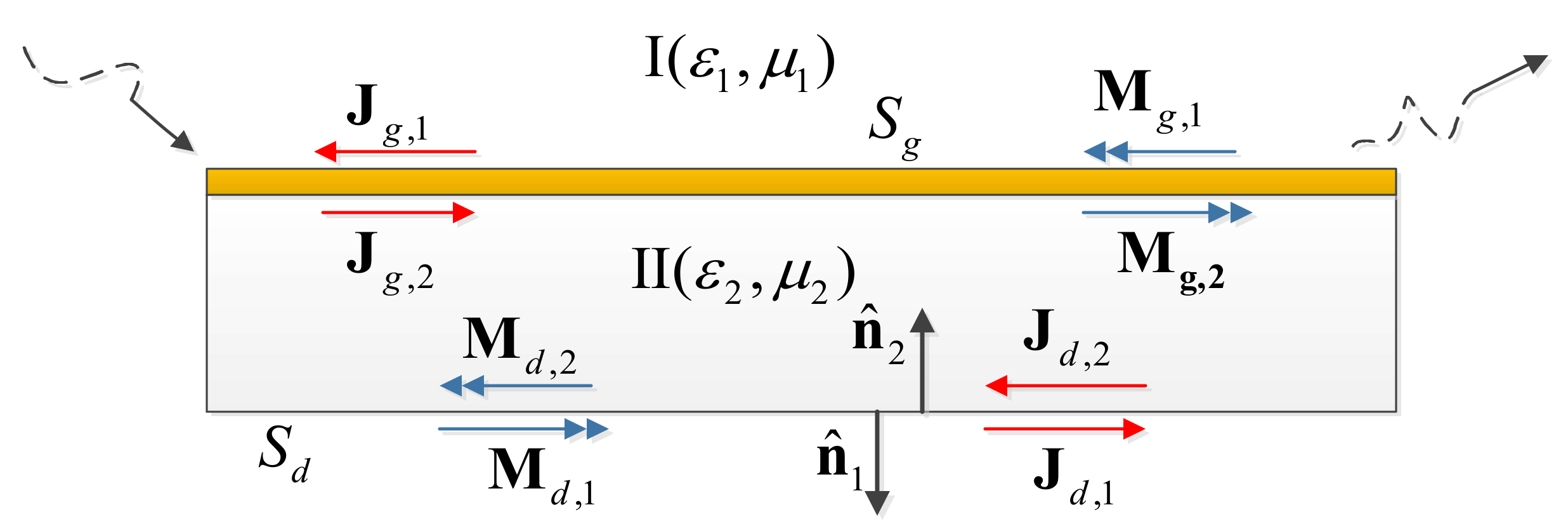
2.1. Integral Equations

The graphene sheet with the dielectric substrate (Domain II: constitutive parameters permittivity ε₂ and permeability μ₂) resides in a background medium (Domain I: constitutive parameters permittivity ε₁ and permeability μ₁) (Figure 1). The excitation electromagnetic field is {Eⁱ(r,t), Hⁱ(r,t)}. In the text below, subscripts g and d indicate graphene and dielectric substrate, and subscript l = 1 or 2 indicates the domain I or II. S = S_g∪S_d represents the closed surface of the composite structure, and ∪ denotes union operation. By using the equivalence principle, the time domain integral equation is formulated with the induced/equivalent electric and magnetic currents and on the surface S, viz. J_l(r,t) = J_g,l(r,t)∪J_d,l(r,t) and M_l(r,t) = M_g,l(r,t)∪M_d,l(r,t). The surface electric and magnetic currents generate the scattered fields. Enforcing the time domain resistive boundary condition (TD-RBC) [14,15,16,34,35,36] of total tangential electric and magnetic fields, the time domain integral equations are established on S:

$$-{\widehat{\mathit{n}}}_l(\mathit{r})\times {\widehat{\mathit{n}}}_l(\mathit{r})\times \left[{\eta }_l{\mathcal{L}}_l({\mathit{J}}_l)+{\mathcal{K}}_l({\mathit{M}}_l)-{\mathit{E}}_l^i(\mathit{r},t)\right]=-{\widehat{\mathit{n}}}_l(\mathit{r})\times {\mathit{M}}_l(\mathit{r},t)$$

(1)

$$-{\widehat{\mathit{n}}}_l(\mathit{r})\times {\widehat{\mathit{n}}}_l(\mathit{r})\times \left[{\eta }_l{}^{-1}{\mathcal{L}}_l({\mathit{M}}_l)+{\mathcal{K}}_l({\mathit{J}}_l)-H_l^i(\mathit{r},t)\right]={\widehat{\mathit{n}}}_l(\mathit{r})\times {\mathit{J}}_l(\mathit{r},t)$$

(2)

The integral operators ${\mathcal{L}}_l$(X) and ${\mathcal{K}}_l$(X) are

$${\mathcal{L}}_l(\mathit{X})=\frac{1}{4\mathsf{\pi }{c}_l}{\displaystyle {\int }_S{\partial }_t\left[\mathit{X}({\mathit{r}}^{\prime },t-\frac{R}{c_l})/R\right]}d{S}^{\prime }+\frac{c_l}{4\mathsf{\pi }}\nabla {\displaystyle {\int }_S{\displaystyle {\int }_{-\infty }^{t-\frac{R}{c}}\left[{\nabla }^{\prime }\cdot \mathit{X}({\mathit{r}}^{\prime },t^{\prime })/R\right]d{t}^{\prime }}}d{S}^{\prime }$$

(3)

$${\mathcal{K}}_l(\mathit{X})=\frac{1}{4\mathsf{\pi }}\nabla \times {\displaystyle {\int }_S\left[\mathit{X}({\mathit{r}}^{\prime },t-\frac{R}{c_l})/R\right]}d{S}^{\prime }$$

(4)

where the intrinsic impedance ${\eta }_l=\sqrt{{\mathsf{\mu }}_l/{\mathsf{\epsilon }}_l}$, speed of electromagnetic waves $c_l=1/\sqrt{{\mathsf{\mu }}_l{\mathsf{\epsilon }}_l}$, retarded time t′ = t − R/$c_l$, ${\widehat{\mathit{n}}}_l(\mathit{r})$ is the unit normal vector, r and r′ are observation and source point position vectors, and R = |r − r′| is the distance.

The resistive boundary condition on S_g is

$$R(t)\ast \left[{\mathit{J}}_{g,1}(\mathit{r},t)+{\mathit{J}}_{g,2}(\mathit{r},t)\right]=\widehat{\mathit{n}}(\mathit{r})\times {\mathit{M}}_{g,l}(\mathit{r},t)$$

(5)

$$\sigma (t)\ast {\mathit{M}}_{g,1}(\mathit{r},t)=-\widehat{\mathit{n}}(\mathit{r})\times \left[{\mathit{J}}_{g,1}(\mathit{r},t)+{\mathit{J}}_{g,2}(\mathit{r},t)\right]$$

(6)

where $\ast$ is temporal convolution, and R(t) and σ(t) are surface resistivity and conductivity of graphene in the time domain, respectively. On S_g, M_g,1 = −M_g,2, but J_g,1 ≠ −J_g,2. On S_d, J_d,1 = −J_d,2 and M_d,1 = –M_d,2. For simplification, let J_d = J_d,1 = −J_d,2, J_g = J_g,1, J_r = J_g,2, M_g = M_g,1 = −M_g,2, and M_d = M_d,1 = −M_d,2. Substituting Equations (1) and (2) into (5) and (6), then, one obtains:

$$-R(t)\ast ({\mathit{J}}_g+{\mathit{J}}_{\mathit{r}})+{\eta }_1{\mathcal{L}}_1({\mathit{J}}_d+{\mathit{J}}_g)+{\mathcal{K}}_1({\mathit{M}}_d+{\mathit{M}}_g)={\mathit{E}}^i(\mathit{r},t)$$

(7)

$$R(t)\ast ({\mathit{J}}_g+{\mathit{J}}_{\mathit{r}})+{\eta }_2{\mathcal{L}}_2({\mathit{J}}_d-{\mathit{J}}_{\mathit{r}})+{\mathcal{K}}_2({\mathit{M}}_d+{\mathit{M}}_g)=0$$

(8)

$$-\sigma (t)\ast {\mathit{M}}_g+{\eta }_1{}^{-1}{\mathcal{L}}_1({\mathit{M}}_d+{\mathit{M}}_g)+{\eta }_2{}^{-1}{\mathcal{L}}_2({\mathit{M}}_d+{\mathit{M}}_g)-{\mathcal{K}}_1({\mathit{J}}_d+{\mathit{J}}_g)-{\mathcal{K}}_2({\mathit{J}}_d-{\mathit{J}}_{\mathit{r}})={\mathit{H}}^i(\mathit{r},t)$$

(9)

Enforcing the continuity of the tangential electric and magnetic field components, the time domain PMCHW formulation on S_d is:

$${\eta }_1{\mathcal{L}}_1({\mathit{J}}_d+{\mathit{J}}_g)+{\eta }_2{\mathcal{L}}_2({\mathit{J}}_d-{\mathit{J}}_{\mathit{r}})+{\mathcal{K}}_1({\mathit{M}}_d+{\mathit{M}}_g)+{\mathcal{K}}_2({\mathit{M}}_d+{\mathit{M}}_g)={\mathit{E}}^i(\mathit{r},t)$$

(10)

$${\eta }_1{}^{-1}{\mathcal{L}}_1({\mathit{M}}_d+{\mathit{M}}_g)+{\eta }_2{}^{-1}{\mathcal{L}}_2({\mathit{M}}_d+{\mathit{M}}_g)-{\mathcal{K}}_1({\mathit{J}}_d+{\mathit{J}}_g)-{\mathcal{K}}_2({\mathit{J}}_d-{\mathit{J}}_{\mathit{r}})={\mathit{H}}^i(\mathit{r},t)$$

(11)

Equations (7)–(11) are coupled and solved to determine the unknown electric and magnetic currents J_g, J_d, J_r, M_g, and M_d.

2.2. MOD Scheme

The surface S is modeled with triangle patches. The electric current (the magnetic current can be obtained similarly) is expressed as:

$$\mathit{J}\left(\mathit{r},t\right)={\displaystyle \sum _{n=1}^{N_S}\left({\displaystyle \sum _{j=0}^{N_L}{J}_{n,j}{\mathsf{\phi }}_j\left(t\right)}\right){\mathit{f}}_n\left(r\right)}$$

(12)

where $J_{n,j}$ is the unknown coefficient, ${\mathit{f}}_n\left(\mathit{r}\right)$ is the spatial basis function (the well-known RWG basis function over triangular patches), and the temporal basis function ${\mathsf{\phi }}_j\left(t\right)$ is the weighted Laguerre polynomial (WLP) of j-th degree [29,31,32,33]. The WLP is defined on zero to +∞ and is convergent to zero as time passes. Hence, it is suitable to be a temporal basis function in the transient problem.

The j-th degree Laguerre polynomial is:

$$L_j\left(t\right)=\frac{\exp \left(t\right)}{j!}\frac{d^j}{d{t}^j}\left(t^j\exp \left(-t\right)\right), 0\le t<\infty$$

(13)

The Laguerre polynomials are orthogonal with respect to the weight:

$${\displaystyle \underset{0}{\overset{\infty }{\int }}\exp (-t)L_i\left(t\right)L_j\left(t\right)}dt={\mathsf{\delta }}_{ij}$$

(14)

where ${\mathsf{\delta }}_{ij}$ is a Kronecker delta. If i = j, ${\mathsf{\delta }}_{ij}$ = 1; if i ≠ j, ${\mathsf{\delta }}_{ij}$ = 0.

The WLP is

$${\mathsf{\phi }}_j(t)=\exp \left(-st/2\right)L_j\left(st\right)$$

(15)

where s is the temporal scaling factor. By choosing an appropriate temporal scaling factor s, viz. increasing or decreasing the support of the WLP, the transient electromagnetic responses can be approximated accurately.

Multilayer graphene’s frequency domain surface resistivity/conductivity computed by the Kubo formula [22,23,24] can be tuned by number of layers, operation frequency, chemical potential, scattering rate (relaxation time), and temperature. The vector fitting method approximates the dispersive frequency domain graphene surface resistivity/conductivity using several pairs of complex conjugate poles and residues as:

$$\mathsf{\rho }\left(\mathsf{\omega }\right)={\displaystyle \sum _{v=1}^p\frac{d_v}{j\mathsf{\omega }-a_v}}$$

(16)

$$\mathsf{\sigma }\left(\mathsf{\omega }\right)={\displaystyle \sum _{v=1}^p\frac{{d_v}^{\prime }}{j\mathsf{\omega }-{a_v}^{\prime }}}$$

(17)

where ω is the angular frequency. The real parts of poles a_v and a_v′ should be negative.

By inverse Fourier transform, graphene’s time domain surface resistivity/conductivity is

$$\mathsf{\rho }\left(t\right)=u\left(t\right){\displaystyle \sum _{v=1}^p{d}_v\exp \left(a_{v}t\right)}$$

(18)

$$\mathsf{\sigma }\left(t\right)=u\left(t\right){\displaystyle \sum _{v=1}^p{d_v}^{\prime }\exp \left({a_v}^{\prime }t\right)}$$

(19)

where u(t) is the unit step function.

In order to facilitate the numerical computation, we make use of new source vectors ${\mathit{e}}_d(\mathit{r},t)$,${\mathit{e}}_g(\mathit{r},t)$, ${\mathit{e}}_{\mathit{r}}(\mathit{r},t)$, ${\mathit{h}}_d(\mathit{r},t)$, and ${\mathit{h}}_g(\mathit{r},t)$, and for example, we define ${\mathit{e}}_d(\mathit{r},t)={\displaystyle \sum _{n=1}^{N_s}{e}_n^d(t){\mathit{f}}_n(\mathit{r})}$, ${\mathit{h}}_d(\mathit{r},t)={\displaystyle \sum _{n=1}^{N_s}{h}_n^d(t){\mathit{f}}_n(r)}$.

Take ${\mathit{e}}_d(\mathit{r},t)$, for example, in further detail below, we define [29,31]:

$${\mathit{e}}_d(\mathit{r},t)={\displaystyle \sum _{n=1}^{N_s}{e}_n^d(t){\mathit{f}}_n(r)}={\displaystyle \sum _{n=1}^{N_s}{\displaystyle \sum _{j=0}^{N_L}{e}_{n,j}^d}{\mathsf{\phi }}_j(t){\mathit{f}}_n(r)}$$

(20)

Therefore,

$${\mathit{J}}_d(\mathit{r},t)=\frac{\partial }{\partial t}{\mathit{e}}_d(\mathit{r},t)={\displaystyle \sum _{n=1}^{N_s}\left(s{\displaystyle \sum _{j=0}^{N_L}\left(\frac{1}{2}{e}_{n,j}^d+{\displaystyle \sum _{k=0}^{j-1}{e}_{n,k}^d}\right)}{\mathsf{\phi }}_j\left(t\right)\right)}{\mathit{f}}_n(\mathit{r})$$

(21)

$$\frac{\partial }{\partial t}{\mathit{J}}_d(\mathit{r},t)=\frac{{\partial }^2}{\partial t^2}{\mathit{e}}_d(\mathit{r},t)={\displaystyle \sum _{n=1}^{N_s}\left(s^2{\displaystyle \sum _{j=0}^{N_L}\left(\frac{1}{4}{e}_{n,j}^d+{\displaystyle \sum _{k=0}^{j-1}\left(i-k\right)e_{n,k}^d}\right)}{\mathsf{\phi }}_j\left(t\right)\right)}{\mathit{f}}_n(\mathit{r})$$

(22)

After the spatial and temporal test following the Galerkin method (both the spatial and temporal basis functions are the same as the testing functions), convert the coupled time domain integral equations to the matrix form as:

$$\left[\left.\begin{array}{cccc}{\mathsf{\alpha }}_{{}_{mn}}^{\left(1\right)}& {\mathsf{\beta }}_{mn}^{\left(1\right)}& {\mathsf{\gamma }}_{mn}^{\left(1\right)}& \begin{array}{cc}{\mathsf{\lambda }}_{mn}^{\left(1\right)}& {\mathsf{\chi }}_{mn}^{\left(1\right)}\end{array}\\ {\mathsf{\alpha }}_{{}_{mn}}^{\left(2\right)}& {\mathsf{\beta }}_{mn}^{\left(2\right)}& {\mathsf{\gamma }}_{mn}^{\left(2\right)}& \begin{array}{cc}{\mathsf{\lambda }}_{mn}^{\left(2\right)}& {\mathsf{\chi }}_{mn}^{\left(2\right)}\end{array}\\ {\mathsf{\alpha }}_{{}_{mn}}^{\left(3\right)}& {\mathsf{\beta }}_{mn}^{\left(3\right)}& {\mathsf{\gamma }}_{mn}^{\left(3\right)}& \begin{array}{cc}{\mathsf{\lambda }}_{mn}^{\left(3\right)}& {\mathsf{\chi }}_{mn}^{\left(3\right)}\end{array}\\ \begin{array}{c}{\mathsf{\alpha }}_{{}_{mn}}^{\left(4\right)}\\ {\mathsf{\alpha }}_{{}_{mn}}^{\left(5\right)}\end{array}& \begin{array}{c}{\mathsf{\beta }}_{mn}^{\left(4\right)}\\ {\mathsf{\beta }}_{mn}^{\left(5\right)}\end{array}& \begin{array}{c}{\mathsf{\gamma }}_{mn}^{\left(4\right)}\\ {\mathsf{\gamma }}_{mn}^{\left(5\right)}\end{array}& \begin{array}{c}\begin{array}{cc}{\mathsf{\lambda }}_{mn}^{\left(4\right)}& {\mathsf{\chi }}_{mn}^{\left(4\right)}\end{array}\\ \begin{array}{cc}{\mathsf{\lambda }}_{mn}^{\left(5\right)}& {\mathsf{\chi }}_{mn}^{\left(5\right)}\end{array}\end{array}\end{array}\right]\right.\left[\left.\begin{array}{c}{e}_{n,i}^d\\ e_{n,i}^g\\ e_{n,i}^{\mathit{r}}\\ \begin{array}{c}{h}_{n,i}^d\\ h_{n,i}^g\end{array}\end{array}\right]\right.=\left[\begin{array}{c}\begin{array}{c}{V}_{m,j}^{\left(1\right),inc}+V_{m,j}^{\left(1\right)}\\ V_{m,j}^{\left(2\right),inc}+V_{m,j}^{\left(2\right)}\end{array}\\ V_{m,j}^{\left(3\right),inc}+V_{m,j}^{\left(3\right)}\\ V_{m,j}^{\left(4\right),inc}+V_{m,j}^{\left(4\right)}\\ V_{m,j}^{\left(5\right),inc}+V_{m,j}^{\left(5\right)}\end{array}\right]$$

(23)

where

$$\begin{array}{cc}\hfill & {\mathsf{\alpha }}_{mn}^{\left(1\right)}=\sum _{l=1}^2\left(\frac{s^2}{4}{\mathsf{\mu }}_l{A}_{mn}+\frac{1}{{\mathsf{\epsilon }}_1}{\mathsf{\varphi }}_{mn}\right)exp\left(\frac{-s{R}_{mn}}{2c_l}\right)\hfill \\ \hfill & {\mathsf{\alpha }}_{mn}^{\left(2\right)}=-\sum _{l=1}^2\left(\frac{s^2{I}_1}{4}\frac{1}{c_l}+s{I}_2\right)exp\left(\frac{-s{R}_{mn}}{2c_l}\right)\hfill \\ \hfill & {\mathsf{\alpha }}_{mn}^{\left(3\right)}=\sum _{l=1}^2\left(\frac{s^2}{4}{\mathsf{\mu }}_1{A}_{mn}+\frac{1}{{\mathsf{\epsilon }}_1}{\mathsf{\varphi }}_{mn}\right)exp\left(\frac{-s{R}_{mn}}{2c_l}\right)\hfill \\ \hfill & {\mathsf{\alpha }}_{mn}^{\left(4\right)}=\sum _{l=1}^2\left(\frac{s^2}{4}{\mathsf{\mu }}_2{A}_{mn}+\frac{1}{{\mathsf{\epsilon }}_2}{\mathsf{\varphi }}_{mn}\right)exp\left(\frac{-s{R}_{mn}}{2c_l}\right)\hfill \\ \hfill & {\mathsf{\alpha }}_{mn}^{\left(5\right)}=\sum _{l=1}^2\left(\frac{s^2{I}_1}{4}\frac{1}{c_l}+s{I}_2\right)exp\left(\frac{-s{R}_{mn}}{2c_l}\right)\hfill \end{array}$$

(24)

$$\begin{array}{cc}\hfill & {\mathsf{\beta }}_{mn}^{\left(1\right)}=\left(\frac{s^2}{4}{\mathsf{\mu }}_1{A}_{mn}+\frac{1}{{\mathsf{\epsilon }}_1}{\mathsf{\varphi }}_{mn}\right)exp\left(\frac{-s{R}_{mn}}{2c_1}\right)\hfill \\ \hfill & {\mathsf{\beta }}_{mn}^{\left(2\right)}=\frac{s}{2}{q}_{mn}-\left(\frac{s^2}{4}\frac{I_1}{c_1}+\frac{s}{2}{I}_2\right)exp\left(\frac{-s{R}_{mn}}{2c_1}\right)\hfill \\ \hfill & {\mathsf{\beta }}_{mn}^{\left(3\right)}=\left(\frac{s^2}{4}{\mathsf{\mu }}_1{A}_{mn}+\frac{1}{{\mathsf{\epsilon }}_1}{\mathsf{\varphi }}_{mn}-\frac{1}{s}\sum _{v=1}^p\frac{-d_v}{(1+b_v)b_v}\right)exp\left(\frac{-s{R}_{mn}}{2c_1}\right)\hfill \\ \hfill & {\mathsf{\beta }}_{mn}^{\left(4\right)}=\left(\frac{1}{s}\sum _{v=1}^p\frac{-d_v}{(1+b_v)b_v}\right)exp\left(\frac{-s{R}_{mn}}{2c_1}\right)\hfill \\ \hfill & {\mathsf{\beta }}_{mn}^{\left(5\right)}=\frac{s}{2}{q}_{mn}+\left(\frac{s^2}{4}\frac{I_1}{c_1}+\frac{s}{2}{I}_2\right)exp\left(\frac{-s{R}_{mn}}{2c_1}\right)\hfill \end{array}$$

(25)

$$\begin{array}{cc}\hfill & {\mathsf{\gamma }}_{mn}^{\left(1\right)}=-\left(\frac{s^2}{4}{\mathsf{\mu }}_2{A}_{mn}+\frac{1}{{\mathsf{\epsilon }}_2}{\mathsf{\varphi }}_{mn}\right)exp\left(\frac{-s{R}_{mn}}{2c_2}\right)\hfill \\ \hfill & {\mathsf{\gamma }}_{mn}^{\left(2\right)}=\frac{s}{2}{q}_{mn}+\left(\frac{s^2}{4}\frac{I_1}{c_2}+\frac{s}{2}{I}_2\right)exp\left(\frac{-s{R}_{mn}}{2c_2}\right)\hfill \\ \hfill & {\mathsf{\gamma }}_{mn}^{\left(3\right)}=\left(-\frac{1}{s}\sum _{v=1}^p\frac{-d_v}{(1+b_v)b_v}\right)exp\left(\frac{-s{R}_{mn}}{2c_2}\right)\hfill \\ \hfill & {\mathsf{\gamma }}_{mn}^{\left(4\right)}=\left(\frac{1}{s}\sum _{v=1}^p\frac{-d_v}{(1+b_v)b_v}-\frac{s^2}{4}{\mathsf{\mu }}_2{A}_{mn}-\frac{1}{{\mathsf{\epsilon }}_2}{\mathsf{\varphi }}_{mn}\right)exp\left(\frac{-s{R}_{mn}}{2c_2}\right)\hfill \\ \hfill & {\mathsf{\gamma }}_{mn}^{\left(5\right)}=q_{mn}+\left(\frac{s^2}{4}\frac{I_1}{c_2}+\frac{s}{2}{I}_2\right)exp\left(\frac{-s{R}_{mn}}{2c_2}\right)\hfill \end{array}$$

(26)

$$\begin{array}{cc}\hfill & {\mathsf{\lambda }}_{mn}^{\left(1\right)}={\mathsf{\chi }}_{mn}^{\left(1\right)}=\sum _{l=1}^2\left[\frac{s^2{I}_1}{4}\frac{1}{c_l}+s{I}_2\right]exp\left(\frac{-s{R}_{mn}}{2c_l}\right)\hfill \\ \hfill & {\mathsf{\lambda }}_{mn}^{\left(2\right)}={\mathsf{\chi }}_{mn}^{\left(2\right)}=\sum _{l=1}^2\left(\frac{s^2}{4}{\mathsf{\epsilon }}_l{A}_{mn}+\frac{1}{{\mathsf{\mu }}_l}{\mathsf{\varphi }}_{mn}\right)exp\left(\frac{-s{R}_{mn}}{2c_l}\right)\hfill \\ \hfill & {\mathsf{\lambda }}_{mn}^{\left(3\right)}={\mathsf{\chi }}_{mn}^{\left(3\right)}=\frac{s}{2}{q}_{mn}+\sum _{l=1}^2\left(\frac{s^2}{4}\frac{I_1}{c_1}+\frac{s}{2}{I}_2\right)exp\left(\frac{-s{R}_{mn}}{2c_l}\right)\hfill \\ \hfill & {\mathsf{\lambda }}_{mn}^{\left(4\right)}={\mathsf{\chi }}_{mn}^{\left(4\right)}=\sum _{l=1}^2\left(\frac{s^2}{4}\frac{I_1}{c_2}+\frac{s}{2}{I}_2\right)exp\left(\frac{-s{R}_{mn}}{2c_l}\right)-\frac{s}{2}{q}_{mn}\hfill \\ \hfill & {\mathsf{\lambda }}_{mn}^{\left(5\right)}=\sum _{l=1}^2\left(\frac{s^2}{4}{\mathsf{\epsilon }}_l{A}_{mn}+\frac{1}{{\mathsf{\mu }}_l}{\mathsf{\varphi }}_{mn}\right)exp\left(\frac{-s{R}_{mn}}{2c_l}\right)\hfill \\ \hfill & {\mathsf{\chi }}_{mn}^{\left(5\right)}=\sum _{l=1}^2\left(\frac{s^2}{4}{\mathsf{\epsilon }}_l{A}_{mn}+\frac{1}{{\mathsf{\mu }}_l}{\mathsf{\varphi }}_{mn}-\frac{1}{s}\sum _{v=1}^p\frac{-{d_v}^{\prime }}{(1+{b_v}^{\prime }){b_v}^{\prime }}\right)exp\left(\frac{-s{R}_{mn}}{2c_l}\right)\hfill \end{array}$$

(27)

$$V_{m,j}^{(1),inc}=V_{m,j}^{(3),inc}={\displaystyle \int V_m^E(t){\mathsf{\phi }}_j(t)\mathrm{d}t}$$

(28)

$$V_{m,j}^{(2),inc}=V_{m,j}^{(5),inc}={\displaystyle \int V_m^H(t){\mathsf{\phi }}_j(t)\mathrm{d}t}$$

(29)

$$V_{m,j}^{(4),inc}=0$$

(30)

$$\begin{array}{cc}\hfill V_{m,i}^{\left(1\right)}=& -\sum _{l=1}^2\sum _{j=0}^{i-1}\left\{\begin{array}{c}{s}^2{A}_{mn}\left[{\mathsf{\mu }}_1\left[\frac{e_{n,j}^d+e_{n,j}^g}{4}+\sum _{k=0}^{j-1}(j-k)(e_{n,k}^d+e_{n,k}^g)\right]+{\mathsf{\mu }}_2\left[\frac{e_{n,j}^d-e_{n,j}^R}{4}+\sum _{k=0}^{j-1}(j-k)(e_{n,k}^d-e_{n,k}^R)\right]\right]\hfill \\ +{\mathsf{\varphi }}_{mn}\left[\frac{1}{{\mathsf{\epsilon }}_1}\left(e_{n,j}^d+e_{n,j}^g\right)+\frac{1}{{\mathsf{\epsilon }}_2}\left(e_{n,j}^d-e_{n,j}^R\right)\right]\hfill \\ +\frac{I_1{s}^2}{c_l}\left[\frac{h_{n,j}^d+h_{n,j}^g}{4}+\sum _{k=0}^{j-1}(j-k)(h_{n,k}^d+h_{n,k}^g)\right]+s{I}_2\left[\frac{h_{n,j}^d+h_{n,j}^g}{2}+\sum _{k=0}^{j-1}\left(h_{n,k}^d+h_{n,k}^g\right)\right]\hfill \end{array}\right\}{\mathsf{\phi }}_{i,j}\left(\frac{R_{mn}}{c_l}\right)\hfill \\ & -\sum _{l=1}^2\left\{\begin{array}{c}{s}^2{A}_{mn}\left[{\mathsf{\mu }}_1\sum _{k=0}^{i-1}(i-k)(e_{n,k}^d+e_{n,k}^g)+{\mathsf{\mu }}_2\sum _{k=0}^{i-1}(i-k)(e_{n,k}^d-e_{n,k}^r)\right]\hfill \\ +\frac{I_1{s}^2}{c_l}(i-k)\sum _{k=0}^{i-1}(h_{n,k}^d+h_{n,k}^g)+s{I}_2\sum _{k=0}^{i-1}\left(h_{n,k}^d+h_{n,k}^g\right)\hfill \end{array}\right\}exp\left(\frac{-s{R}_{mn}}{2c_l}\right)\hfill \end{array}$$

(31)

$$\begin{array}{cc}\hfill V_{m,i}^{\left(2\right)}=& \sum _{j=0}^{i-1}\left[\frac{s}{2}{G}_{mn}\sum _{k=0}^{j-1}\left(e_{n,k}^g+e_{n,k}^r\right)\right]-\frac{s}{2}{G}_{mn}\sum _{k=0}^{i-1}\left(e_{n,k}^g+e_{n,k}^r\right)\hfill \\ & -\sum _{j=0}^{i-1}\left\{\begin{array}{c}{\mathsf{\epsilon }}_1{s}^2{A}_{mn}\left[\frac{h_{n,j}^d+h_{n,j}^g}{4}+\sum _{k=0}^{j-1}(j-k)(h_{n,k}^d+h_{n,k}^g)\right]+\frac{1}{{\mathsf{\mu }}_1}{\mathsf{\varphi }}_{mn}\left(h_{n,j}^d+h_{n,j}^g\right)\hfill \\ -\frac{I_1{s}^2}{c_1}\left[\frac{e_{n,j}^d+e_{n,j}^g}{4}+\sum _{k=0}^{j-1}(j-k)(e_{n,k}^d+e_{n,k}^g)\right]-s{I}_2\left[\frac{e_{n,j}^d+e_{n,j}^g}{2}+\sum _{k=0}^{j-1}(e_{n,k}^d+e_{n,k}^g)\right]\hfill \\ -\frac{I_1{s}^2}{c_2}\left[\frac{e_{n,j}^d-e_{n,j}^r}{4}+\sum _{k=0}^{j-1}(j-k)(e_{n,k}^d-e_{n,k}^r)\right]-s{I}_2\left[\frac{e_{n,j}^d-e_{n,j}^r}{2}+\sum _{k=0}^{j-1}(e_{n,k}^d-e_{n,k}^r)\right]\hfill \end{array}\right\}{\mathsf{\phi }}_{i,j}\left(\frac{R_{mn}}{c_1}\right)\hfill \\ & -\left\{\begin{array}{c}{\mathsf{\epsilon }}_1{s}^2{A}_{mn}\sum _{k=0}^{i-1}(i-k)(h_{n,k}^d+h_{n,k}^g)\hfill \\ -\frac{I_1{s}^2}{c_1}\sum _{k=0}^{i-1}(i-k)(e_{n,k}^d+e_{n,k}^g)-s{I}_2\sum _{k=0}^{i-1}(e_{n,k}^d+e_{n,k}^g)\hfill \\ -\frac{I_1{s}^2}{c_2}\sum _{k=0}^{i-1}(i-k)(e_{n,k}^d-e_{n,k}^r)-s{I}_2\sum _{k=0}^{i-1}(e_{n,k}^d-e_{n,k}^r)\hfill \end{array}\right\}exp\left(\frac{-s{R}_{mn}}{2c_1}\right)\hfill \end{array}$$

(32)

$$\begin{array}{cc}\hfill V_{m,i}^{\left(3\right)}=& -\sum _{j=0}^{i-1}\left\{\begin{array}{c}{\mathsf{\mu }}_1{s}^2{A}_{mn}\left[\frac{e_{n,j}^d+e_{n,j}^g}{4}+\sum _{k=0}^{j-1}(j-k)(e_{n,k}^d+e_{n,k}^g)\right]+\frac{1}{{\mathsf{\epsilon }}_1}{\mathsf{\varphi }}_{mn}\left(e_{n,j}^d+e_{n,j}^g\right)\hfill \\ +\frac{I_1{s}^2}{c_1}\left[\frac{h_{n,j}^d+h_{n,j}^g}{4}+\sum _{k=0}^{j-1}(j-k)(h_{n,k}^d+h_{n,k}^g)\right]\hfill \\ +s{I}_2\left[\frac{h_{n,j}^d+h_{n,j}^g}{2}+\sum _{k=0}^{j-1}(h_{n,k}^d+h_{n,k}^g)\right]\hfill \\ -\frac{1}{s}{G}_{mn}\sum _{k=0}^j\left[(e_{n,k}^r+e_{n,k}^g)\sum _{v=1}^p\frac{-d_v}{(1+b_v)b_v}{\left(1+\frac{1}{b_v}\right)}^{j-k}\right]\hfill \end{array}\right\}{\mathsf{\phi }}_{i,j}\left(\frac{R_{mn}}{c_2}\right)\hfill \\ & -\left\{\begin{array}{c}{\mathsf{\mu }}_1{s}^2{A}_{mn}\sum _{k=0}^{i-1}(i-k)(e_{n,k}^d+e_{n,k}^g)\hfill \\ +\frac{I_1{s}^2}{c_1}\sum _{k=0}^{i-1}(i-k)(h_{n,k}^d+h_{n,k}^g)+s{I}_2\sum _{k=0}^{i-1}(h_{n,k}^d+h_{n,k}^g)\hfill \\ -\frac{1}{s}{G}_{mn}\sum _{k=0}^{i-1}\left[(e_{n,k}^r+e_{n,k}^g){\sum _{v=1}^p\frac{-d_v}{(1+b_v)b_v}\left(1+\frac{1}{b_v}\right)}^{i-k}\right]\hfill \end{array}\right\}exp\left(\frac{-s{R}_{mn}}{2c_2}\right)\hfill \end{array}$$

(33)

$$\begin{array}{cc}\hfill V_{m,i}^{\left(4\right)}=& -\sum _{l=1}^2\sum _{j=0}^{i-1}\left\{\begin{array}{c}{\mathsf{\mu }}_2{s}^2{A}_{mn}\left[\frac{e_{n,j}^d-e_{n,j}^r}{4}+\sum _{k=0}^{j-1}(j-k)(e_{n,k}^d-e_{n,k}^r)\right]+\frac{1}{{\mathsf{\epsilon }}_2}{\mathsf{\varphi }}_{mn}\left(e_{n,j}^d-e_{n,j}^r\right)\hfill \\ +\frac{I_1{s}^2}{c_2}\left[\frac{h_{n,j}^d+h_{n,j}^g}{4}+\sum _{k=0}^{j-1}(j-k)(h_{n,k}^d+h_{n,k}^g)\right]\hfill \\ +s{I}_2\left[\frac{h_{n,j}^d+h_{n,j}^g}{2}+\sum _{k=0}^{j-1}(h_{n,k}^d+h_{n,k}^g)\right]\hfill \\ +\frac{1}{s}{G}_{mn}\sum _{k=0}^j\left[(e_{n,k}^r+e_{n,k}^g)\sum _{v=1}^p\frac{-d_v}{(1+b_v)b_v}{\left(1+\frac{1}{b_v}\right)}^{j-k}\right]\hfill \end{array}\right\}{\mathsf{\phi }}_{i,j}\left(\frac{R_{mn}}{c_l}\right)\hfill \\ & -\sum _{l=1}^2\left\{\begin{array}{c}{\mathsf{\mu }}_2{s}^2{A}_{mn}\sum _{k=0}^{i-1}(e_{n,k}^d-e_{n,k}^r)\hfill \\ +\frac{I_1{s}^2}{c_2}\sum _{k=0}^{i-1}(i-k)(h_{n,k}^d+h_{n,k}^g)+s{I}_2\sum _{k=0}^{i-1}(h_{n,k}^d+h_{n,k}^g)\hfill \\ +\frac{1}{s}{G}_{mn}\sum _{k=0}^{i-1}\left[(e_{n,k}^r+e_{n,k}^g)\sum _{v=1}^p\frac{-d_v}{(1+b_v)b_v}{\left(1+\frac{1}{b_v}\right)}^{i-k}\right]\hfill \end{array}\right\}exp\left(\frac{-s{R}_{mn}}{2c_l}\right)\hfill \end{array}$$

(34)

$$\begin{array}{cc}\hfill V_{m,i}^{\left(5\right)}=& -\sum _{l=1}^2\sum _{j=0}^{i-1}\left\{\begin{array}{c}{\mathsf{\epsilon }}_l{s}^2{A}_{mn}\left[\frac{h_{n,j}^d+h_{n,j}^g}{4}+\sum _{k=0}^{j-1}(j-k)(h_{n,k}^d+h_{n,k}^g)\right]+\frac{1}{{\mathsf{\mu }}_l}{\mathsf{\varphi }}_{mn}\left(h_{n,j}^d+h_{n,j}^g\right)\hfill \\ -\frac{I_1{s}^2}{c_1}\left[\frac{e_{n,j}^d+e_{n,j}^g}{4}+\sum _{k=0}^{j-1}(j-k)(e_{n,k}^d+e_{n,k}^g)\right]-s{I}_2\left[\frac{e_{n,j}^d+e_{n,j}^g}{2}+\sum _{k=0}^{j-1}(e_{n,k}^d+e_{n,k}^g)\right]\hfill \\ -\frac{I_1{s}^2}{c_2}\left[\frac{e_{n,j}^d-e_{n,j}^r}{4}+\sum _{k=0}^{j-1}(j-k)(e_{n,k}^d-e_{n,k}^r)\right]-s{I}_2\left[\frac{e_{n,j}^d-e_{n,j}^r}{2}+\sum _{k=0}^{j-1}(e_{n,k}^d-e_{n,k}^r)\right]\hfill \\ -\frac{1}{s}{G}_{mn}\left[\sum _{k=0}^j{h}_{n,k}^g{\sum _{v=1}^p\frac{-{d_v}^{\prime }}{(1+{b_v}^{\prime }){b_v}^{\prime }}\left(1+\frac{1}{b_v}\right)}^{j-k}\right]\hfill \end{array}\right\}{\mathsf{\phi }}_{i,j}\left(\frac{R_{mn}}{c_l}\right)\hfill \\ & -\sum _{l=1}^2\left\{\begin{array}{c}{\mathsf{\epsilon }}_l{s}^2{A}_{mn}\sum _{k=0}^{i-1}(i-k)(h_{n,k}^d+h_{n,k}^g)-\frac{I_1{s}^2}{c_1}\sum _{k=0}^{i-1}(j-k)(e_{n,k}^d+e_{n,k}^g)\hfill \\ -s{I}_2\sum _{k=0}^{i-1}(e_{n,k}^d+e_{n,k}^g)-\frac{I_1{s}^2}{c_2}\sum _{k=0}^{i-1}(j-k)(e_{n,k}^d-e_{n,k}^R)\hfill \\ -s{I}_2\sum _{k=0}^{i-1}(e_{n,k}^d-e_{n,k}^R)-\frac{1}{s}{G}_{mn}\left[\sum _{k=0}^{i-1}{h}_{n,k}^g{\sum _{v=1}^p\frac{-{d_v}^{\prime }}{(1+{b_v}^{\prime }){b_v}^{\prime }}\left(1+\frac{1}{b_v}\right)}^{i-k}\right]\hfill \end{array}\right\}exp\left(\frac{-s{R}_{mn}}{2c_l}\right)\hfill \end{array}$$

(35)

and

$${\mathsf{\phi }}_{i,j}\left(t\right)={\mathsf{\phi }}_{i-j}\left(t\right)-{\mathsf{\phi }}_{i-j-1}\left(t\right)$$

(36)

$$A_{mn}=\frac{1}{4\mathsf{\pi }}{\displaystyle \int {\mathit{f}}_m\left(\mathit{r}\right){\displaystyle \int \frac{{\mathit{f}}_n\left({\mathit{r}}^{\prime }\right)}{R}}}\mathrm{d}{S}^{\prime }\mathrm{d}S$$

(37)

$${\mathsf{\varphi }}_{mn}=\frac{1}{4\mathsf{\pi }}{\displaystyle \int \nabla \cdot {\mathit{f}}_m\left(\mathit{r}\right){\displaystyle \int \frac{{\nabla }^{\prime }\cdot {\mathit{f}}_n\left({\mathit{r}}^{\prime }\right)}{R}}}\mathrm{d}{S}^{\prime }\mathrm{d}S$$

(38)

$$I_v=\frac{1}{4\mathsf{\pi }}{\displaystyle \int {\mathit{f}}_m\left(\mathit{r}\right)\cdot \widehat{n}\times {\displaystyle \int {\mathit{f}}_n\left({\mathit{r}}^{\prime }\right)\times \frac{\widehat{\mathit{R}}}{{\left(R_{mn}\right)}^v}}}\mathrm{d}{S}^{\prime }\mathrm{d}S,v=1,2$$

(39)

$$G_{mn}={\displaystyle \int {\mathit{f}}_m\left(\mathit{r}\right)\cdot {\mathit{f}}_n\left({\mathit{r}}^{\prime }\right)}\mathrm{d}S$$

(40)

b_v = a_v/s–1/2, b_v′ = a_v′/s–1/2

(41)

where R_mn is the distance between centroids of the two triangles related to ${\mathit{f}}_m\left(\mathit{r}\right)$ and ${\mathit{f}}_n\left({\mathit{r}}^{\prime }\right)$.

The matrix Equation (23) is solved by increasing the degree of the WLP, and the surface current can be obtained, from which the radar cross section (RCS), extinction cross section (ECS), etc., can be computed.

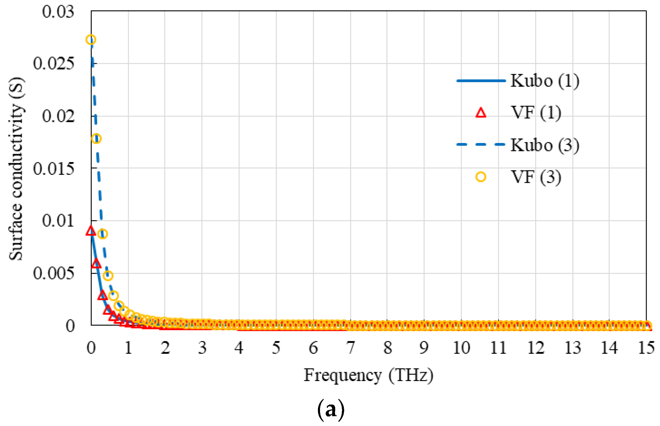
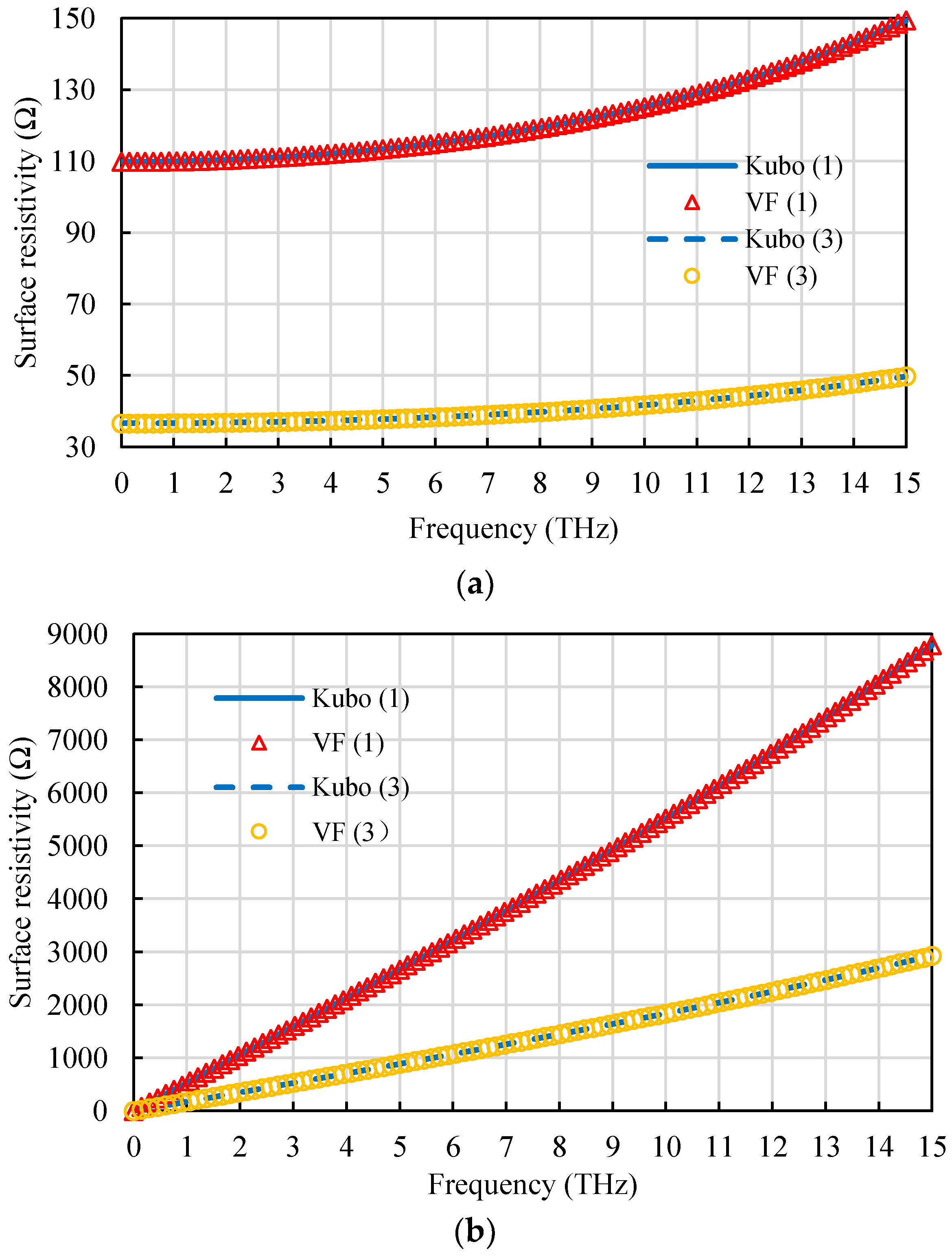
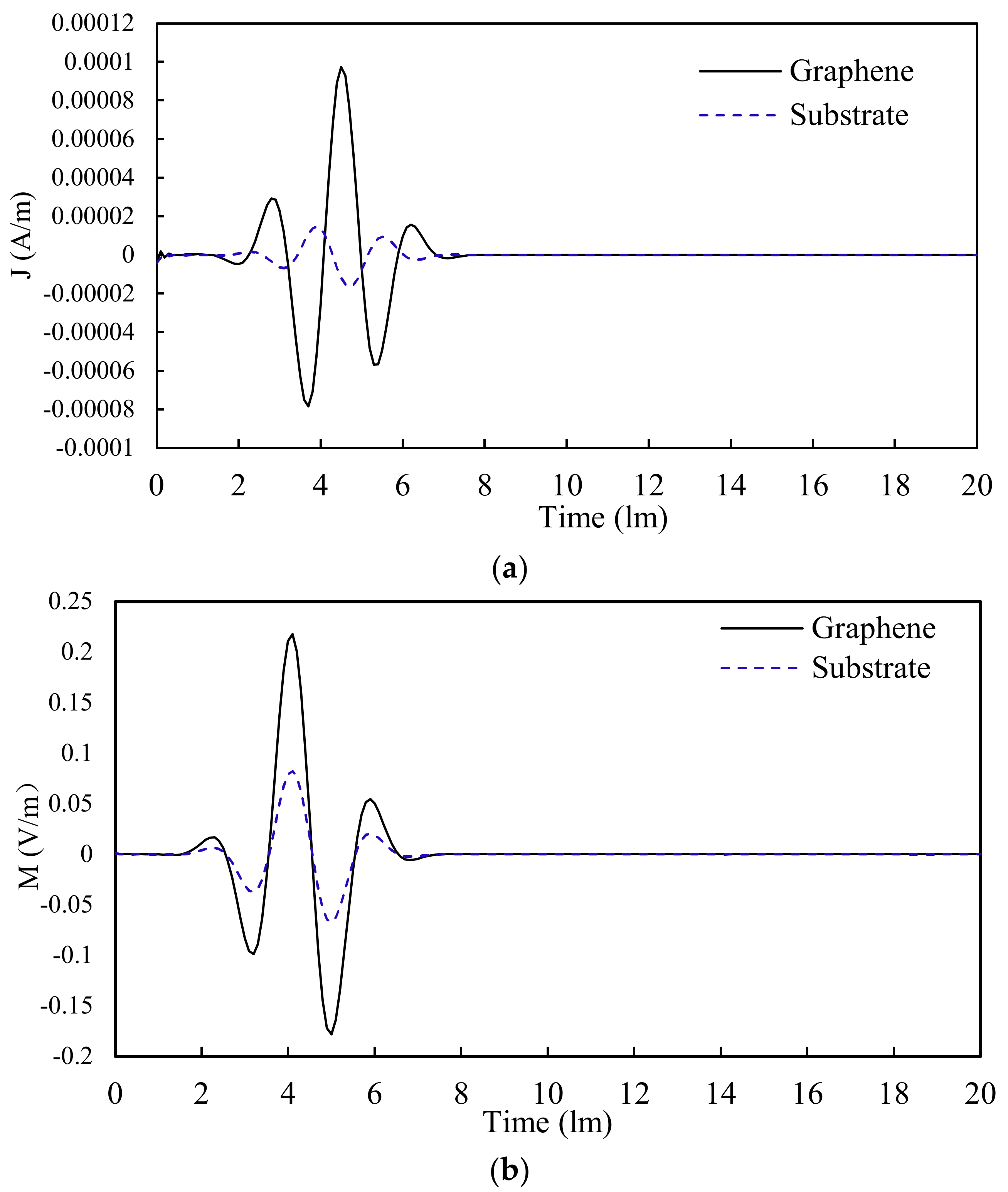
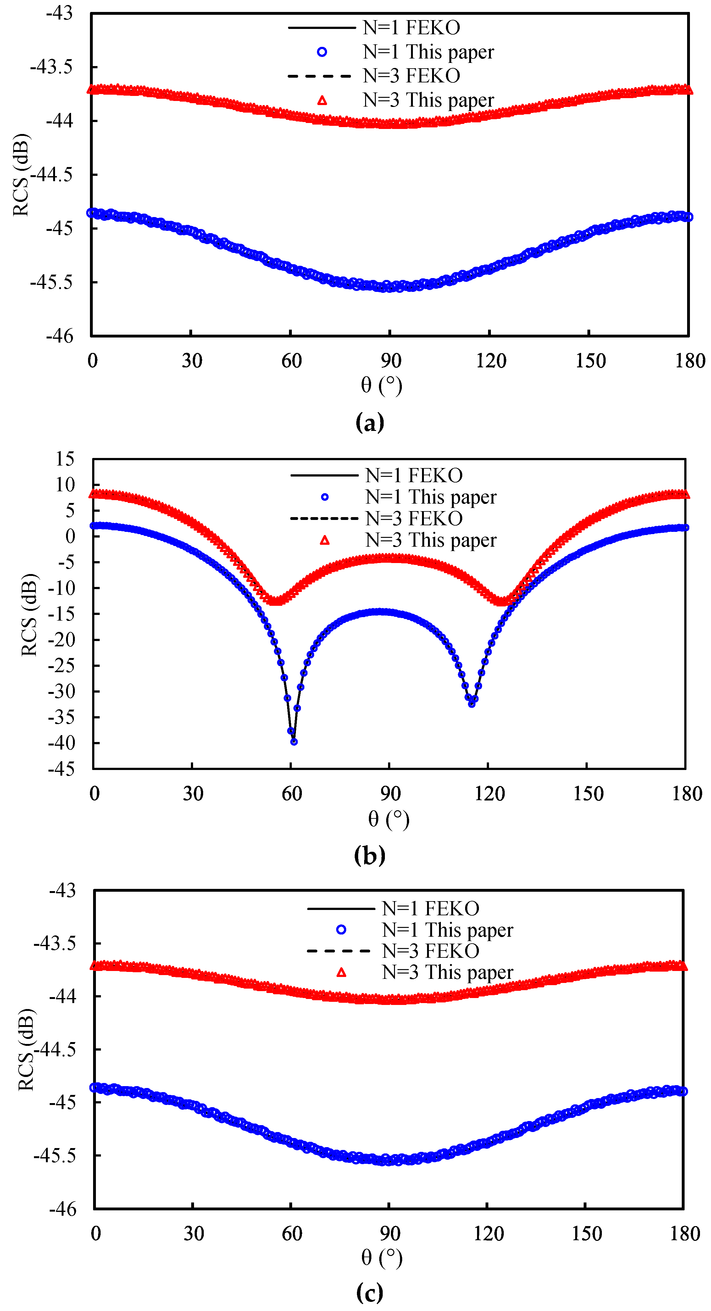
3. Results and Discussion

Consider the trilayer 0.02 × 0.04 mm² graphene (chemical potential μ_c = 0.1 eV, scattering rate Γ = 0.43 meV/ℏ, ℏ is reduced Plank constant, temperature T = 300 K) with the ZnO substrate (relative permittivity is 3.61, thickness is 0.003 mm). The lower surface of the dielectric substrate is centered at the coordinate origin (Figure 2). The surface conductivity and resistivity of trilayer graphene from 0.1 to 15 THz computed by the Kubo formula are approximated with VF (Figure 3 and Figure 4). Three pairs of poles and residues, listed in

Table 1. a_v′ and d_v′ of trilayer graphene surface conductivity.

v	av′	dv′
1	−0.0131 × 1014	3.5680 × 1010
2, 3	(–0.0132 ± j5.1838) × 1014	5.1373 × 1010 ± j9.1549 × 105

and

Table 2. a_v and dv of trilayer graphene surface resistivity.

v	av	dv
1	−1.3983 × 1015	1.0143 × 1017
2, 3	(–0.0026 ± j0.2995) × 1015	(1.2579 ± j0.0161) × 1018

, can achieve satisfactory accuracy.

The incident excitation is the modulated Gaussian pulse defined by

$${\mathit{E}}^i\left(\mathit{r},t\right)=\widehat{\mathit{x}}\cos \left(2\mathsf{\pi }{f}_0\tau \right)\exp \left(-\frac{{\left(\tau -t_p\right)}^2}{2t_w{}^2}\right)$$

(42)

$${\mathit{H}}^i\left(\mathit{r},t\right)=\frac{1}{120\mathsf{\pi }}\widehat{\mathit{k}}\times {\mathit{E}}^i\left(\mathit{r},t\right)$$

(43)

The central frequency f₀ is 7.2 THz, $\tau =t-r\cdot \widehat{\mathit{k}}/c$, $\widehat{\mathit{k}}$ is the incident unit vector, and along the –z direction in this example, t_p = 3.5 t_w is the time delay of the peak from t = 0, pulse width t_w = 3/(2πf₀).

The trilayer graphene with the ZnO substrate is analyzed using the MOD method developed in Section 2 with 50 WLPs. The graphene and dielectric substrate are meshed by 240 triangles. The scaling factor s is 7.5 × 10¹⁰.

End points of two randomly chosen inner edges on upper surface of graphene and lower surface of dielectric substrate are (0.003905 × 10⁻³, 0.009757 × 10⁻³, 0.003 × 10⁻³), (0.007851 × 10⁻³, 0.011957 × 10⁻³, 0.003 × 10⁻³) and (0.003953 × 10⁻³, 0.009599 × 10⁻³, 0), (0.008007 × 10⁻³, 0.011579 × 10⁻³, 0). The transient current across the two inner edges is shown in Figure 5. One light meter (lm) equals approximately 3.33 ns. The current is stable and convergent.

Furthermore, the wide frequency band information can be obtained after the Fourier transform of the time domain solution. The example results of the bistatic radar cross section (RCS) at 1.06, 7.2, and 12.9 THz agree well with those obtained via FEKO in Figure 6 (N = 1 and N = 3 denote monolayer and trilayer graphene). θ and φ are the elevation angles and azimuth angles, respectively. Besides, the extinction cross section (ECS) [37], which is more interesting at THz and optical frequencies, is displayed and compared with the COMSOL simulation in Figure 7. It shows good agreement between the two curves.

4. Conclusions

As subsequent work of the authors, transient electromagnetic analysis of multilayer graphene with a dielectric substrate is performed in this paper. Multilayer graphene’s dispersive surface conductivity/resistivity is tackled by convolution of temporal surface conductivity/resistivity and magnetic/electric current densities. The TD-RBC integral equation and the time domain PMCHW equation are established and coupled together, then, solved in the MOD scheme. Using convergent weighted Laguerre polynomials, the time variable is eliminated, and stable transient solution is obtained. Radar cross section and extinction cross section compared with commercial software in the wide band also verify the proposed method. A more complex dielectric substrate, e.g., vanadium dioxide (VO2), and multi-physics transient electromagnetic-thermal coupled field problems will be studied in the future.

References

1. Zhao, Y.T.; Wu, B.; Huang, B.J.; Cheng, Q. Switchable broadband terahertz absorber/reflector enabled by hybrid graphene-gold metasurface. Opt. Express 2017, 25, 7161–7169. [Google Scholar] [CrossRef] [PubMed]
2. Vakil, A. Transformation Optics Using Graphene: One-Atom-Thick Optical Devices Based on Graphene. Ph.D. Thesis, University of Pennsylvania, Philadelphia, PA, USA, 2012. [Google Scholar]
3. Tsai, H.Y.; Hsu, W.H.; Liao, Y.J. Effect of electrode coating with graphene suspension on power generation of microbial fuel cells. Coatings 2018, 8, 243. [Google Scholar] [CrossRef] [Green Version]
4. Kyhl, L.; Nielsen, S.F.; Čabo, A.G.; Cassidy, A.; Miwa, J.A.; Hornekær, L. Graphene as an anti-corrosion coating layer. Faraday Discuss. 2015, 180, 495–509. [Google Scholar] [CrossRef] [PubMed]
5. Tsai, P.Y.; Chen, T.E.; Lee, Y.L. Development and characterization of anticorrosion and antifriction properties for high performance polyurethane/graphene composite coatings. Coatings 2018, 8, 250. [Google Scholar] [CrossRef] [Green Version]
6. Chen, L.; Zhang, Y.; Wu, Q. Effect of graphene coating on the heat transfer performance of a composite anti-/deicing component. Coatings 2017, 7, 158. [Google Scholar] [CrossRef]
7. Gong, F.; Li, H.; Wang, W.; Xia, D.; Liu, Q.; Papavassiliou, D.V.; Xu, Z. Recent advances in graphene-based free-standing films for thermal management: Synthesis, properties, and applications. Coatings 2018, 8, 63. [Google Scholar] [CrossRef] [Green Version]
8. Hsu, A.R.; Chien, H.H.; Liao, C.Y.; Lee, C.C.; Tsai, J.H.; Hsu, C.C.; Cheng, I.; Chen, J.Z. Scan-mode atmospheric-pressure plasma jet processed reduced graphene oxides for quasi-solid-state gel-electrolyte supercapacitors. Coatings 2018, 8, 52. [Google Scholar] [CrossRef] [Green Version]
9. Shen, B.; Li, Y.; Yi, D.; Zhai, W.T.; Wei, X.C.; Zheng, W.G. Strong flexible polymer/graphene composite films with 3D saw-tooth folding for enhanced and tunable electromagnetic shielding. Carbon 2017, 113, 55–62. [Google Scholar] [CrossRef]
10. Qiao, Y.C.; Wang, Y.F.; Tian, H.; Li, M.R.; Jian, J.M.; Wei, Y.H.; Tian, Y.; Wang, D.Y.; Pang, Y.; Geng, X.; et al. Multilayer graphene epidermal electronic skin. ACS Nano 2018, 12, 8839–8846. [Google Scholar] [CrossRef]
11. Lin, H.; Pantoja, M.F.; Angulo, L.D.; Alvarez, J.; Martin, R.G.; Garcia, S.G. FDTD modeling of graphene devices using complex conjugate dispersion material model. IEEE Microw. Wirel. Compon. Lett. 2012, 22, 612–614. [Google Scholar] [CrossRef]
12. Nayyeri, V.; Soleimani, M.; Ramahi, O.M. Wideband modeling of graphene using the finite-difference time-domain method. IEEE Trans. Antennas Propag. 2013, 61, 6107–6114. [Google Scholar] [CrossRef]
13. Wang, D.W.; Zhao, W.S.; Gu, X.Q.; Chen, W.C.; Yin, W.Y. Wideband modeling of graphene-based structures at different temperatures using hybrid FDTD method. IEEE Trans. Nanotechnol. 2015, 14, 250–258. [Google Scholar] [CrossRef]
14. Li, P.; Jiang, L.J.; Bağci, H. A resistive boundary condition enhanced DGTD scheme for the transient analysis of graphene. IEEE Trans. Antennas Propag. 2015, 63, 3065–3076. [Google Scholar] [CrossRef] [Green Version]
15. Li, P.; Jiang, L.J. Modeling of magnetized graphene from microwave to THz range by DGTD with a scalar RBC and an ADE. IEEE Trans. Antennas Propag. 2015, 63, 4458–4467. [Google Scholar] [CrossRef] [Green Version]
16. Shi, Y.F.; Uysal, I.E.; Li, P.; Ulku, H.A.; Bağci, H. Analysis of electromagnetic wave interactions on graphene sheets using time domain integral equations. In Proceedings of the International ACES Conference, Williamsburg, VA, USA, 22–26 March 2015. [Google Scholar]
17. Shi, Y.F.; Li, P.; Uysal, I.E.; Ulku, H.A.; Bağci, H. An MOT-TDIE solver for analyzing transient fields on graphene-based devices. In Proceedings of the IEEE International Symposium Antennas Propagation (APSURSI), Fajardo, Puerto Rico, 26 June–1 July 2016. [Google Scholar]
18. Wang, Q.Q.; Liu, H.Z.; Wang, Y.; Jiang, Z.N. Marching-on-in-degree time-domain integral equation solver for transient electromagnetic analysis of graphene. Coatings 2017, 7, 170. [Google Scholar] [CrossRef] [Green Version]
19. Abergel, D.S.L.; Russell, A.; Fal’ko, V.I. Visibility of graphene flakes on a dielectric substrate. Appl. Phys. Lett. 2007, 91, 063125. [Google Scholar] [CrossRef] [Green Version]
20. Craciun, M.F.; Russo, S.; Yamamoto, M.; Tarucha, S. Tuneable electronic properties in graphene. Nano Today 2011, 6, 42–60. [Google Scholar] [CrossRef] [Green Version]
21. McCann, E.; Koshino, M. The electronic properties of bilayer graphene. Rep. Prog. Phys. 2013, 76, 056503. [Google Scholar] [CrossRef]
22. Lin, I.T. Optical Properties of Graphene from the THz to the Visible Spectral Region. Master’s Thesis, University of California, Los Angeles, CA, USA, 2012. [Google Scholar]
23. Du, W.; Hao, R.; Li, E.P. The study of few-layer graphene based Mach-Zehnder modulator. Opt. Commun. 2014, 323, 49–53. [Google Scholar] [CrossRef]
24. Wang, Q.Q.; Shi, Y.; Liu, H.Z. Modeling of multilayer graphene at terahertz with vector fitting method. In Proceedings of the International Conference on Systems and Informatics (ICSAI), Nanjing, China, 10–12 November 2018; pp. 780–784. [Google Scholar]
25. Gustavsen, B.; Semlyen, A. Rational approximation of frequency domain responses by vector fitting. IEEE Trans. Power Deliv. 1999, 14, 1052–1061. [Google Scholar] [CrossRef] [Green Version]
26. Gustavsen, B. Improving the pole relocating properties of vector fitting. IEEE Trans. Power Deliv. 2006, 21, 1587–1592. [Google Scholar] [CrossRef]
27. Deschrijver, D.; Gustavsen, B.; Dhaene, T. Advancements in iterative methods for rational approximation in the frequency domain. IEEE Trans. Power Deliv. 2007, 22, 1633–1642. [Google Scholar] [CrossRef]
28. Pordanjani, I.R.; Xu, W. Improvement of vector fitting by using a new method for selection of starting poles. Electr. Power Syst. Res. 2014, 107, 206–212. [Google Scholar] [CrossRef]
29. Jung, B.H.; Sarkar, T.K.; Chung, Y.S. Solution of time domain PMCHW formulation for transient electromagnetic scattering from arbitrarily shaped 3-D dielectric objects. Prog. Electromagn. Res. 2004, 45, 291–312. [Google Scholar] [CrossRef] [Green Version]
30. Zhang, G.H.; Xia, M.Y.; Chan, C.H. Time domain integral equation approach for analysis of transient responses by metallic-dielectric composite bodies. Prog. Electromagn. Res. 2008, 87, 1–14. [Google Scholar] [CrossRef] [Green Version]
31. Mei, Z.C. Solving Time Domain Scattering and Radiation Problems in A Marching-on-in-Degree Technique for Method of Moment. Ph.D. Thesis, Syracuse University, Syracuse, NY, USA, 2014. [Google Scholar]
32. Zhu, M.D.; Sarkar, T.K.; Chen, H. A stabilized marching-on-in-degree scheme for the transient solution of the electric field integral equation. IEEE Trans. Antennas Propag. 2019, 67, 3232–3240. [Google Scholar] [CrossRef]
33. Zhu, M.D.; Sarkar, T.K.; Chen, H.; Wu, Y.Z. On the stability of time-domain magnetic field integral equation using Laguerre functions. IEEE Trans. Antennas Propag. 2019, 67, 3939–3947. [Google Scholar] [CrossRef]
34. Chen, Q.; Lu, M.; Michielssen, E. Integral equation-based analysis of transient scattering from surfaces with an impedance boundary condition. Microw. Opt. Technol. Lett. 2004, 42, 213–220. [Google Scholar] [CrossRef]
35. Shanker, B.; Lu, M.; Yuan, J.; Michielssen, E. TDIE analysis of scattering from composite bodies via exact evaluation of radiation fields. IEEE Trans. Antennas Propag. 2009, 57, 1506–1520. [Google Scholar] [CrossRef]
36. Gibson, W.C. The Method of Moments in Electromagnetics, 2nd ed.; Chapman and Hall/CRC, Taylor and Francis Group: New York, NY, USA, 2014. [Google Scholar]
37. Mishchenko, M.I.; Travis, L.D.; Lacis, A.A. Scattering, Absorption, and Emission of Light by Small Particles, 1st ed.; Cambridge University Press: Cambridge, UK, 2002. [Google Scholar]
Figure 1. Graphene sheet with the dielectric substrate.
Coatings 10 00718 g001
Figure 2. Geometric modeling of the trilayer graphene with the dielectric substrate.
Coatings 10 00718 g002
Figure 3. Monolayer and trilayer graphene surface conductivity: (a) real parts; (b) imaginary parts.
Coatings 10 00718 g003aCoatings 10 00718 g003b
Figure 4. Monolayer and trilayer graphene surface resistivity: (a) real parts; (b) imaginary parts.
Coatings 10 00718 g004
Figure 5. Transient currents across two example inner edges of the graphene and substrate: (a) electrical current; (b) magnetic current.
Coatings 10 00718 g005
Figure 6. φ = 90° RCS: (a) 1.06 THz; (b) 7.2 THz; (c) 12.9 THz.
Coatings 10 00718 g006
Figure 7. ECS of the trilayer graphene with substrate.
Coatings 10 00718 g007