Novel Terahertz Nondestructive Method for Measuring the Thickness of Thin Oxide Scale Using Different Hybrid Machine Learning Models

Abstract

Effective control of the thickness of the hot-rolled oxide scale on the surface of the steel strip is very vital to ensure the surface quality of steel products. Hence, terahertz nondestructive technology was proposed to measure the thickness of thin oxide scale. The finite difference time domain (FDTD) numerical simulation method was employed to obtain the terahertz time-domain simulation data of oxide scale with various thickness (0–15 μm). Added Gaussian white noise with a Signal Nosie Reduction (SNR) of 10 dB was used when simulating real test signals, using four wavelet denoising methods to reduce noise and to compare their effectiveness. Two machine learning algorithms were adopted to set up models to achieve this goal, including the classical back-propagation (BP) neural network algorithm and the novel extreme learning machine (ELM) algorithm. The principal component analysis (PCA) algorithm and particle swarm optimization (PSO) algorithm were combined to reduce the dimensions of the terahertz time-domain data and improve the robustness of the machine learning model. It could be clearly seen that the novel hybrid PCA-PSO-ELM model possessed excellent prediction performance. Finally, this work proposed a novel, convenient, online, nondestructive, noncontact, safety and high-precision thin oxide scale thickness measuring method that could be employed to improve the surface quality of iron and steel products.

1. Introduction

Steel is widely used in modern society and will still be the cornerstone of future industrial development and progress, owing to its rich reserves, low price, excellent mechanical properties, simple smelting, tractable alloying and heat treatment. With the development of global economy, as the dominating steel and iron product, the proportion of flat rolled products will continue to increase [1,2]. During the process of hot rolling and cooling of the strip, the primary, secondary and tertiary oxide coatings are formed on the surface of the strip, this multilayer oxide coating is generally called oxide scale. The structure and composition of the oxide scale are very complex, and vary greatly with factors such as cooling system and curling temperature. There are six types of iron oxides: hematite (α-Fe₂O₃), magnetite (Fe₃O₄, ${\mathrm{Fe}}^{\mathrm{II}}{\mathrm{Fe}}_2^{{}^{\mathrm{III}}}{\mathrm{O}}_4$), maghemite (γ-Fe₂O₃), wüstite (FeO), β-Fe₂O₃ and ε-Fe₂O₃. Among them, β-Fe₂O₃ is a rare compound synthesized in the laboratory; ε-Fe₂O₃ is the transition state between hematite and maghemite; maghemite (γ-Fe₂O₃) is not as stable as α-Fe₂O₃ under natural conditions [3,4,5]. Hot-rolled oxide scale is a hybrid of iron oxides (wüstite, magnetite and hematite), from the perspective of the production process of hot-rolled pickled sheets and cold-rolled sheets, if the attached oxide scale cannot be removed, the hot-rolled strip with the attached oxide scale is directly sent to be rolled, and a series of quality problems will occur; firstly, the oxide scale is pressed into the iron matrix, which directly affects the surface quality of the steel strip and is not conducive to subsequent processing, seriously, it will directly cause the scrap of the plate; secondly, the surface processing accuracy and smoothness of the cold roll are extremely high, the price is expensive, and the direct rolling of the oxide scale will cause damage to the cold rolls; thirdly, the broken oxide scale will enter the emulsion circulation system to shorten the lifetime of the emulsion and circulation equipment. Therefore, to ensure the surface quality and obtain a sheet with excellent processing performance, the oxide scale after hot rolling must be thoroughly removed. For the descaling of hot-rolled sheets, the methods adopted around the world include acid pickling descaling, high-pressure water descaling, rolling descaling and so on [6,7,8,9]. Nevertheless, no matter which descaling method is adopted, all these descaling methods must use destructive thickness testing to determine the best descaling process parameters in advance. Additionally, destructive thickness testing must also be adopted to determine whether the oxide scale on the surface of the strip has been completely removed, however, excessive descaling is not allowed, which will increase the cost of descaling and corrode the plate matrix. Generally, the hot-rolled oxide scale is very thin, and its thickness is normally below a dozen microns. Hence, to measure the thickness of oxide scale nondestructively and accurately, nondestructive testing (NDT) technology is considered to be the best and deal solution to solve this problem.

Research on nondestructive evaluation of thin films and coatings is an important research direction in the field of nondestructive testing, a series of progress has been made in recent years, and a variety of nondestructive testing techniques, such as fluorescence spectrum [10,11,12], X-ray [13,14], infrared [15,16], acoustic emission [17,18], eddy current [19,20], and ultrasonic [21,22], have been developed to evaluate the thin films and coatings. Nevertheless, all these traditional nondestructive testing methods have their own weaknesses. Some are about the detection environment; some are about the material properties of the detected medium; others are about the size of the detected object. For example, luminescence testing put up with the extra element doping and most of them are qualitative tests; the infrared testing results are affected drastically by service environment [23,24]. In allusion to the thickness measuring of oxide scale, all these traditional nondestructive testing methods more or less cannot meet the testing requirements, such as the elevated temperature service environment, the long testing distance, the high demand on the thickness measurement precision and so on.

Recently, as a novel emerging technology, terahertz (THz) technology has been gradually applied to the field of non-destructive testing. Terahertz usually refers to electromagnetic waves with the frequency between 0.1 and 10 THz and a wavelength in the range between 0.03 and 3 mm. Compared with traditional nondestructive testing methods, terahertz has strong penetrability to dielectric materials, and can detect objects under non-destructive, low-radiation, nonionizing, non-contact, and real-time evaluation conditions, with high accuracy and no coupling, which is the vital development trend of future nondestructive testing [25,26]. At present, the research on terahertz technology for nondestructive evaluation has been applied in various fields, including aeroengine [27,28,29,30,31], human security [32,33], food safety [34,35], biopharmaceuticals [36,37], composite materials [38,39] and integrated circuits [40,41], various minor anomalies had been successfully inspected by terahertz nondestructive technology.

The application of the terahertz nondestructive testing method in thickness monitoring has now become one of the most mature technologies in its numerous applications. It can already be used in industrial applications and has attracted wide attention from all parties [42,43,44,45,46]. Hot-rolled oxide scale consist of wüstite, hematite and magnetite, and the wüstite is the chief component among them, and the proportion of wüstite is as high as 58% to 95% under different heat treatment conditions [2,47,48,49]. Previous studies have begun to focus on the characterization of oxide scale on the surface of hot-rolled strips by terahertz non-destructive testing technology and made a series of research results for reference in oxide scale thickness measurement. The terahertz refractive index of various iron oxides was studied. Reference [50] indicates that the refractive index of wüstite is estimated to be 4.7. Reference [51,52] indicates that the refractive index of hematite is estimated to be ~5.5, the value of the refractive index is nearly independent of the frequency. Reference [53] indicates that the refractive index of hematite is depend on the crystal orientation, which lies between 4 and 4.4, and it also indicates that the refractive index of magnetite may reach up to 8.25. Nevertheless, reference [54,55] indicates that the refractive index of magnetite in far infrared region is estimated to be 2.8, hence, the refractive index of magnetite is very likely to lie between 2.8 to 8.25. All in all, in regard to the refractive index of the composite hot-rolled oxide scale, it could be concluded that the real refractive indices of wüstite and hematite oxides are close to each other, and the wüstite is the chief component of oxide scale, hence, the real refractive index of wüstite may be used as a result of the real refractive index of oxide scale. Reference [49] is the first to experimentally show that the value of refractive index n = 4.7 for the oxide scale, and this value is in good agreement with the experimental results in oxide scale thickness estimation. Generally, when the terahertz pulse echo reflection technology is used for coating thickness detection, advanced signal processing techniques (such as windowing function deconvolution technology, sparse deconvolution technology, etc.) are often combined with peak-finding method in the time-domain spectroscopy to find the time-domain feature information corresponding to the thickness, but the minimum thickness value that can be monitored, that is, the depth resolution that can be achieved, is usually limited by the coherence length of the terahertz pulse, hence, the thickness monitoring for the oxide scale is usually inaccurate. Moreover, this method is difficult and has very high demands for technical personnel to pick the peaks, which does not meet the needs of steel production in rapidness, convenience and intelligence.

Machine learning was well applied in the evaluation and prediction performance. It was widely known for its advantages in experimentally difficult and data-rich industrial products [56,57]. In this study, the simulated terahertz time-domain signals were acquired by finite difference time domain (FDTD) numerical simulation method. A theoretical model for terahertz wave simulation of single layer dielectric structure was established. The incident wave was set as the terahertz pulse Gaussian wave that was incident vertically above the oxide scale. To get closer to the real test signal, the Gaussian white noise was used to add noise to the simulated time-domain signal, four noise processing methods were used to reduce noise, and the principal component analysis (PCA) method was applied to reduce the data dimension of these noise-reduced time-domain signals. The signal obtained by dimensionality reduction was used as the input feature during modeling, and finally, a variety of machine learning algorithms and optimization algorithms were used to measure the thin oxide scale thickness.

2. Material and Methods

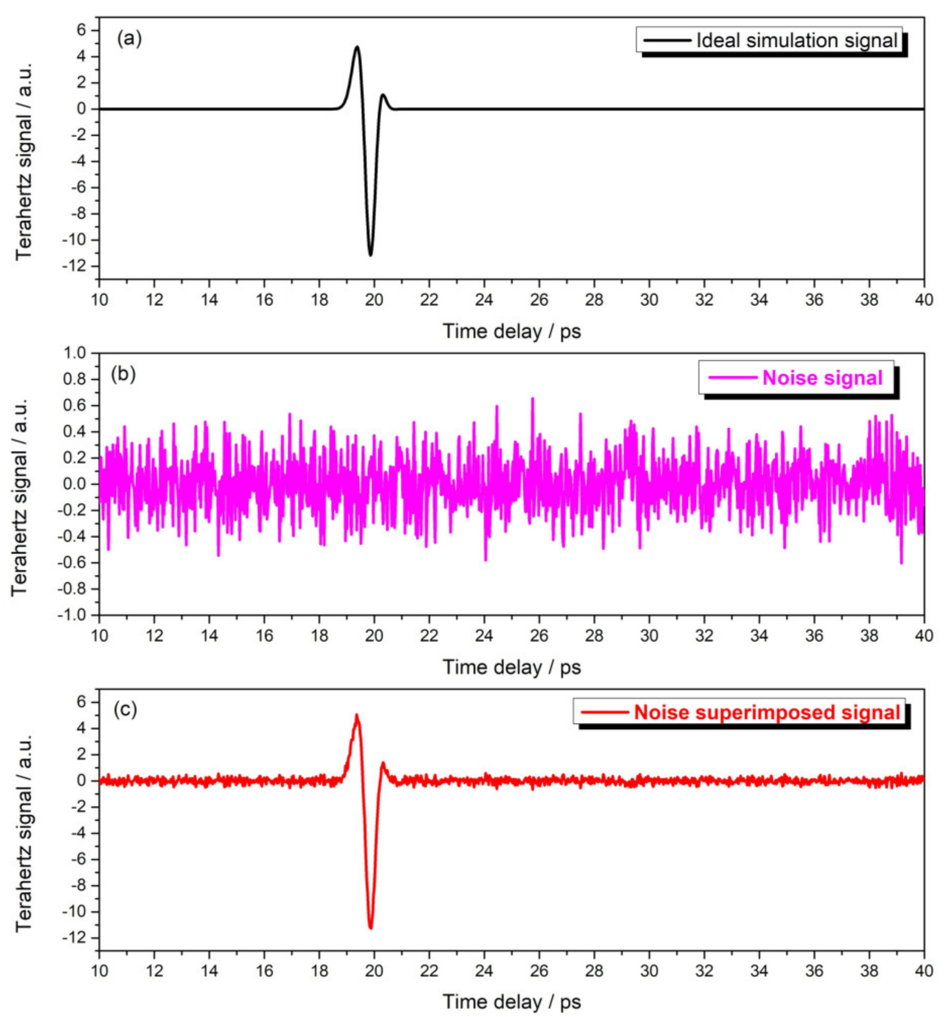
2.1. Terahertz Inspection Signal Obtained by FDTD Simulation

As shown in Figure 1, since the terahertz waves cannot penetrate the metal substrate, it will only reflect on its surface and will not transmit into the metal substrate. A portion of the incident THz waves was reflected on the surface of oxide scale, while a portion of it transmitted through the oxide scale and was absolutely reflected at the interface between the oxide scale and substrate, a portion of the reflected terahertz waves from the interface transmitted through the oxide scale surface into air, and a portion of terahertz waves was reflected back into the oxide scale. Hence, multiple reflection echoes can be received. If the time interval t (t₁, t₂, t₃, t₄, …, t_n) of each reflection can be extracted in the terahertz time-domain spectrum, combined with the refractive index, the thickness of the detected oxide scale can be estimated. Hence, these multiple reflection echoes embodied the thickness message of oxide scale, it is difficult to extract this information, owing to the very thin oxide scale.

The FDTD is based on the vector 3D Maxwell curl equation. The specific connotation of FDTD is that Maxwell’s curl equation is discrete in the time and space domain, and the central differential approximation of the first-order partial derivatives of time and space is used to find the approximate solution of Maxwell’s curl equation [58,59]. In this work, the FDTD Solutions software (Version 8.12.631 for X64, Lumerical Solutions Inc., Vancouver, Canada) was used to model and simulate the propagation process of terahertz waves in oxide scale and analyze the acquired time-domain waveform for detecting the thickness of the oxide scale [44,60]. A batch of simulation models, the oxide scale thickness in these models ranged from 0 to 15 μm (the interval was set as 0.2 μm, there were 76 sets of data), were calculated by the FDTD method, the terahertz waves used was in the frequency range of 0.3–1 THz, and the refractive index of oxide scale was set to 4.7 [49]. Periodic boundary conditions were set in the X and Y directions, and perfectly matched layer (PML) boundary condition was set in the terahertz incidence Z direction [61].

2.2. Signal Nosie Reduction Methods

As shown in Figure 2, for example, the terahertz time domain simulated signal of four samples with different thickness are obtained, with the increase of the thickness, it seems that the oscillations of multiple reflection echoes are getting more and more intense. In fact, unless these oxide scales are thick enough to easily separate multiple echoes from the respective interfaces, and the overlapped echoes cannot be extracted directly even though they embody thickness message. To simulate the real oxide scale monitoring signal in the terahertz frequency band as much as possible, the Gaussian white noise with a Signal Nosie Reduction (SNR) of 10 dB is used to add noise to the simulated time-domain signal. Despite the ideal simulation signal with Gaussian white noise cannot accurately represent the noise oscillation interference in actual test, it is also a common method used in the theoretical study of the terahertz nondestructive testing (NDT) method and is widely used and accepted by researchers [44,62,63].

In this work, four wavelet denoising methods were used to reduce noise: dmey global default threshold for denoising, sym3 wavelet heuristic Stein’S Unbiased Risk Estimation (SURE) threshold denoising, haar wavelet soft SURE threshold denoising, and db3 wavelet fixed threshold denoising (all decomposition levels were set to 5) [64,65]. The sample signal with thickness of 0 was still taken as an example, the residual analysis was performed using the denoised signal and the original unnoisy signal, and the variation of the residual was used to determine which type of noise reduction method was the appropriate noise reduction method, that is, the noise reduction method adopted in this study.

2.3. Modeling Approaches

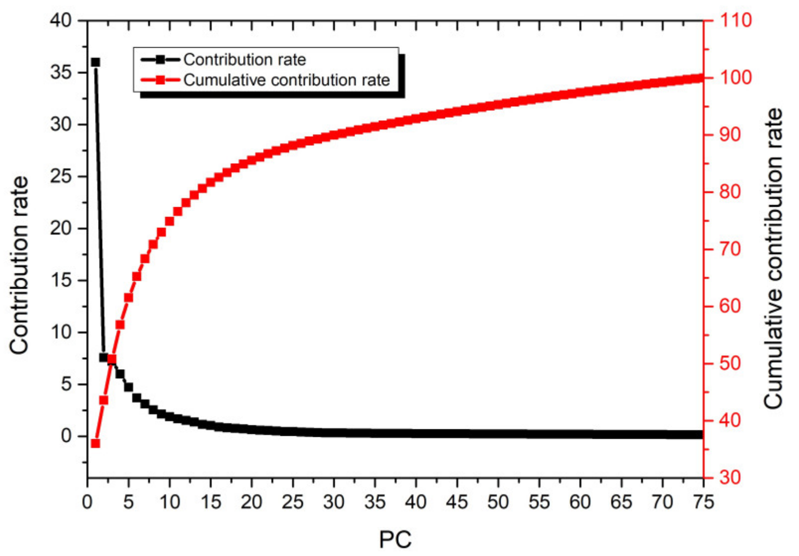
2.3.1. Principal Component Analysis

The principal component analysis (PCA) method is a data analysis method proposed by Pearson more than a century ago. The starting point of the principal component analysis method is to calculate a set of new features arranged in descending order of importance from a set of features. PCA method is to project from a high-dimensional data space to a low-dimensional data space along the direction of maximum covariance, each principal component (PC) obtained is a linear sum of the original variables. The PCs obtained by the PCA are independent of each other, which reduces the dimension of data while ensuring that the loss of original data information is as small as possible. The PCA can not only reduce the dimension of high-dimensional data, but also eliminate the redundant information in high-dimensional data [66].

In this study, the PCA function was implemented through MATLAB programming. The 76 sets of noise-added terahertz time-domain data were denoised by the haar wavelet denoising method. After PCA dimensionality reduction, the eigenvalues, contribution rate and score of each principal component of these haar wavelet denoising signals were obtained. These PCs are used to replace the original terahertz time-domain spectral data as input features during modeling [31].

2.3.2. Back-Propagation Neural Network

The back-propagation (BP) neural network is a forward neural network. The BP neural network can complete the mapping of any dimension through only three layers of neural networks, owing to its simple structure, and it has become the most successful and practical neural network. Almost 80% of the neural networks will prefer the BP neural network when modeling. The BP neural network uses back propagation errors during training, adjusting relevant parameters (such as network weights) to continuously correct the prediction results, and eventually make the prediction results consistent with the actual output. In this continuous iteration process, the error range of the signal is reduced and the accuracy is improved. Therefore, BP neural network has the advantages of simple structure and reliable performance. It can perform self-learning, self-organization and parallel processing of information to realize intelligent prediction, control, process optimization, and fault diagnosis. It has been widely used in many fields. Therefore, this study selected the BP neural network model to predict the thickness of the oxide scale and a three-layer BP neural network was adopted.

For a single hidden layer BP neural network, a total of two transfer functions are required from the input layer to the hidden layer, and the hidden layer to the output layer. The two transfer functions are respectively set to “tansig” and “purelin”. The minimum error of the training target is set to 0.01, and the number of trainings is 1000. The optimal number of neurons of the hidden layer determines the BP neural network training and verification performance. If there are too few nodes in the hidden layer, the robustness of the BP neural network will decrease; if there are too many nodes in the hidden layer, it will lead to too long learning time and “overfitting” phenomenon. There is no clear guiding principle to achieve the optimal prediction performance of the BP neural network, but we can learn from the relevant empirical formulas [67]:

$$K=⌈{\log }_{2}l⌉$$

(1)

where the parameter K and $l$ were the node numbers in the hidden layer and input layer, respectively. In this study, the selected BP neural network topology had 3747 input nodes ($l$ = 12), therefore, the BP neural network was configurated with 12 neurons.

The BP neural network model was trained 50 times using random disordered samples, and the model with minimum validation set error was saved as the prediction model.

2.3.3. Extreme Learning Machine Optimized by Particle Swarm Optimization Algorithm

The extreme learning machine (ELM) is a new type of feed-forward neural network with n training samples ${\left\{\left(x_s,t_s\right)\right\}}_{s=1}^n$($x_s$ is the input vector and $t_s$ is the output vector). Compared with traditional feedforward neural networks, the ELM algorithm randomly generates the connection weights of the input layer and the implicit layer and the thresholds of the implicit layer neurons, and it does not need to be adjusted during the training process. Compared with the previous traditional training methods, the ELM method has the advantages of fast learning speed and good generalization performance. An ELM regression model containing m hidden layer neuron functions $f(\cdot )$ can be expressed as follows [68,69]:

$$\left\{\begin{array}{l}{\displaystyle \sum _{i=1}^m{\mathsf{\omega }}^{\mathrm{T}}}f\left(w_{\mathrm{in}}{x}_1+b_i\right)=t_1\hfill \\ {\displaystyle \sum _{i=1}^m{\mathsf{\omega }}^{\mathrm{T}}}f\left(w_{\mathrm{in}}{x}_2+b_i\right)=t_2\hfill \\ ⋮\hfill \\ {\displaystyle \sum _{i=1}^m{\mathsf{\omega }}^{\mathrm{T}}}f\left(w_{\mathrm{in}}{x}_s+b_i\right)=t_s\hfill \end{array}\right.$$

(2)

where s is the number of training samples; $w_{\mathrm{in}}$ is the input weight of input node and hidden layer node; ω is the output weight value connecting the hidden layer and the output layer; $b_i$ is the deviation of the i-th neuron, that is, the hidden layer threshold. Equation (2) can be converted to matrix form, which can be expressed as follows:

$$HW=T$$

(3)

$$H={\left[\begin{array}{ccc}f\left(w_{\mathrm{in}}{x}_1+b_1\right)& \cdots & f\left(w_{\mathrm{in}}{x}_1+b_l\right)\\ ⋮& & ⋮\\ f\left(w_{\mathrm{in}}{x}_n+b_1\right)& \cdots & f\left(w_{\mathrm{in}}{x}_n+b_l\right)\end{array}\right]}_{N\times l}$$

(4)

$$W={\left[{\mathsf{\omega }}_1{,\mathsf{\omega }}_2\cdots {\mathsf{\omega }}_L\right]}^{\mathrm{T}}$$

(5)

here H is the output matrix of the hidden layer of the neural network; W is the output weight; T is the output vector, $T=\left[t_1,t_2\right.{\left.\cdots ,t_k\right]}^{\mathrm{T}}$; Since it is much larger than m in most cases. Then the output weight value can be estimated by Equation (2) and can be expressed as follows:

$$w={\left(H^{\mathrm{T}}H\right)}^{-1}{H}^{\mathrm{T}}T$$

(6)

therefore, the ELM time series prediction model finally obtained after training can be expressed as follows:

$$t={\displaystyle \sum _{i=1}^m{w}_i}f\left(w_{1n}x+b_i\right)$$

(7)

where x is the input of the prediction model and t is the output of the prediction model.

Particle swarm optimization (PSO) is a bionic optimization algorithm proposed by Kennedy and Eberhart in 1995 [70]. Each particle in a cluster of particles represents a possible solution to a problem, and through the simple behavior of individual particles, the information interaction within the cluster achieves the intelligence of problem solving. Because of its simple operation and fast convergence, PSO is widely used in many fields such as function optimization, image processing, and geodesy. In this work, aiming at the shortcomings of the ELM input weights and hidden layer thresholds are randomly determined, the initial search weights and hidden layer thresholds of the ELM are optimized and selected using the particle swarm optimization algorithm, owing to its excellent global search capability. The steps are as follows:

• Initialize the particle swarm, select the appropriate learning factors (c1 and c2), inertia weight, particle dimension D, maximum iteration number K and population size M.
• For computing the single individuals $w$ and $b_i$, the ELM algorithm can calculate the output weight matrix, and use the training samples to calculate the mean square error ($\mathsf{\sigma }={\displaystyle \sum d_i}/(n-1)$, n is the number of measurements, $d_i$ is the deviation of a set of measured values from the average) of the individual of the initial population.
• Set the PSO adaptability $F_i=\mathsf{\sigma }$, compare the values of $F_i$ and p_best in the same iteration, when $F_i$ is greater than p_best, then use $F_i$ instead of p_best, otherwise it will remain unchanged. Then compare the values of $F_i$ and g_best, when $F_i$ is greater than g_best, then use $F_i$ instead of g_best, otherwise it will still remain unchanged. For three conditions: the number of running times is greater than or equal to the maximum number of iterations, the running time is greater than or equal to the longest running time, and the fitness value is less than or equal to the specified threshold. When any one of these three conditions is met, exit the program and return the current optimal individual and fitness.
• The $w$ and $b_i$ corresponding to the optimal fitness are obtained, and the output weight matrix H is calculated by using Equation (4).

2.3.4. Statistical Assessment of Machine Learning Models

In this study, the 55 random samples were employed as the training sets to set up the BP and PCA-PSO-ELM models, and the remaining 21 samples were used as the validation and prediction sets. The reliability and accuracy of the suggested models were assessed using four evaluation indicators objectively, including: root mean square error (RMSE), mean absolute error (MAE), mean absolute percentage error (MAPE), and squared correlation coefficient (R²). Their definitions are as follows:

$$RMSE=\sqrt{{\displaystyle \sum _{i=1}^n{\left(Y_i-{\widehat{Y}}_i\right)}^2}/n}$$

(8)

$$MAE={\displaystyle \sum _{i=1}^n\left|Y_i-{\widehat{Y}}_i\right|}/n$$

(9)

$$MAPE={\displaystyle \sum _{i=1}^n\frac{\left|Y_i-{\widehat{Y}}_i\right|}{Y_i}}/n$$

(10)

$$R^2={\left[\frac{{\displaystyle \sum _{i=1}^n\left({\widehat{Y}}_i-\overline{\widehat{Y}}\right)}\left(Y_i-\overline{Y}\right)}{\sqrt{{\displaystyle \sum _{i=1}^n{\left({\widehat{Y}}_i-\overline{\widehat{Y}}\right)}^2}}\sqrt{{\displaystyle \sum _{i=1}^n{\left(Y_i-\overline{Y}\right)}^2}}}\right]}^2$$

(11)

where n is the sample size, $Y_i$ is the real value of oxide scale thickness, ${\widehat{Y}}_i$ is the predicted value of oxide scale thickness estimated by machine learning model.

3. Results and Discussion

3.1. Comparison of Various Denoising Methods

As shown in Figure 3, the ideal simulation signal is processed by adding noise to obtain a noise superimposed signal, and it is obvious that the noise superimposed signal in Figure 3c is much closer to the measured signal curve obtained in the actual test. Such a signal containing high-frequency noise further increases the difficulty of thickness information extraction in actual data processing.

As shown in Figure 4, the denoised signals Figure 4a–d were obtained by four wavelet denoising methods, residual distributions Figure 4e–h were applied to identify which denoising method was better, it could be seen that the denoising effect of the sym3 wavelet was the worst, and its residual value was the largest. The effects of the other three wavelet denoising methods were excellent, of which haar wavelet denoising method was the best, and the residual obtained by haar wavelet denoising method was the smallest and the residual distribution law was more consistent with the original set noise signal oscillation law. Hence, the haar wavelet denoising method was adopted to perform noise reduction on 76 sets of noise-added data.

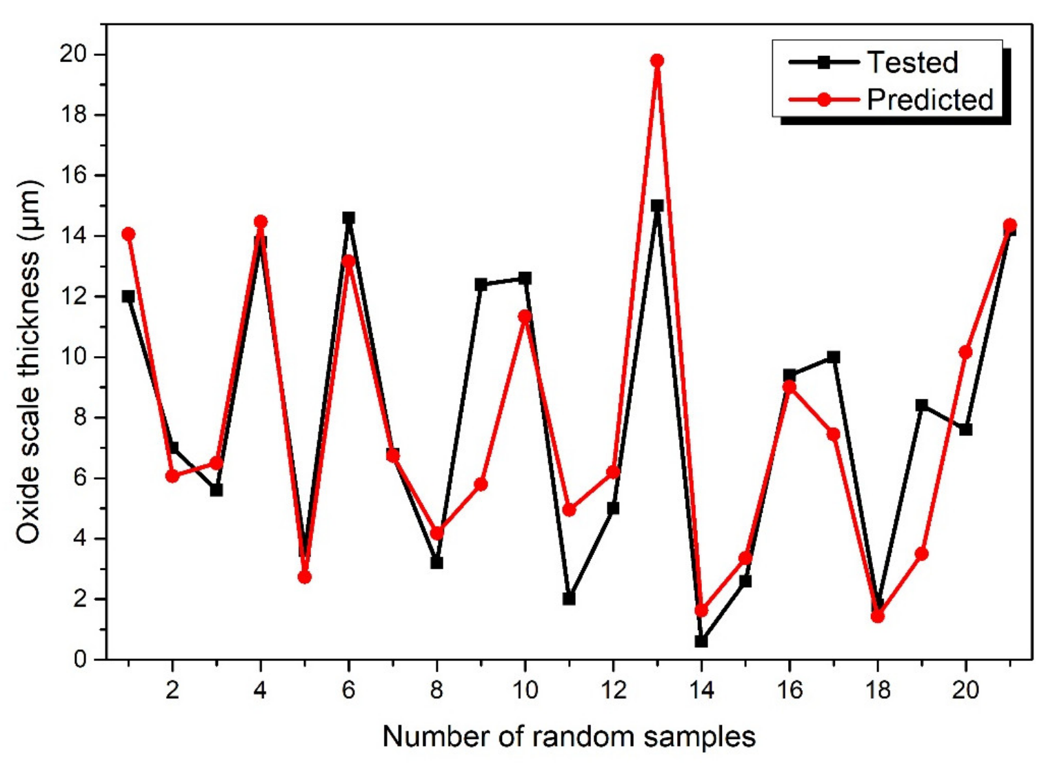
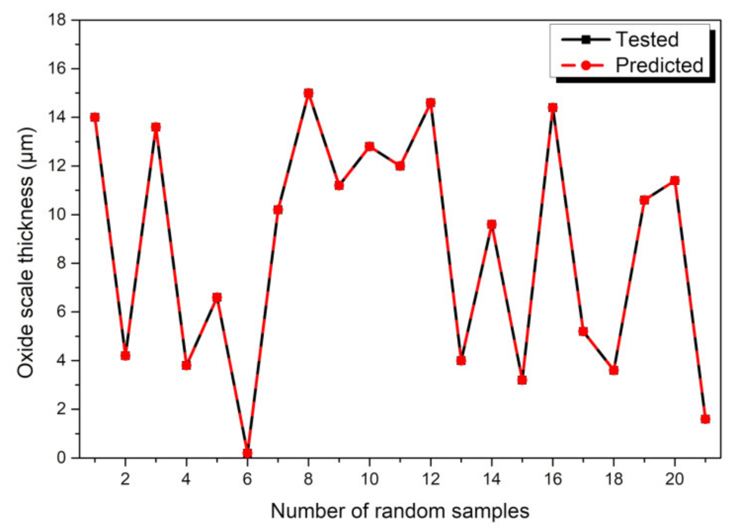
3.2. Comparison of Various Hybrid Machine Learning Approaches

The terahertz time domain data dimension of 76 samples obtained by the FDTD simulation was 76 × 3747. If this large amount of data is directly used for modeling, the calculation speed would be reduced and the accuracy of regression prediction would also be reduced. PCA was used to reduce the dimensions of terahertz time domain data. The eigenvalues of the top three eigenvectors extracted from the terahertz time domain data were 1153.10, 242.91, and 231.47, respectively; as shown in Figure 5, the contribution rates of the top three eigenvectors extracted from the terahertz time domain data were 36.00%, 7.58%, and 7.23%, respectively; the cumulative contribution rate of the first three principal components had exceeded 50%, but the principal component score after the first three principal components was getting lower and lower. Here, in order to make the contribution rate reached 100%, it was found that the cumulative contribution rate of the first 75 principal components was 100%. Finally, the data dimension was reduced from 76 × 3747 to 76 × 75, combined with the eigenvalues and contribution rates above, according to the seventy six-dimensional scores of the top 76 PCs, the top 76 PCs of terahertz time domain data were used as the input to PSO-ELM models for the oxide scale thickness prediction.

For the training results of BP model, to check the reliability and accuracy of the BP model, as shown in Figure 6, it shows comparative results that the training results of the BP model’s target (T, actual value of oxide scale thickness) compared to the BP model’s output (Y, predicted value oxide scale thickness). The linear fitting function curve Y = T in the Figure 6 represents the ideal situation that the predicted value must exactly match the actual value. It can be clearly seen that all the predicted data and actual data are scattered around the Y = T line, their actual linear fitting function curve is Y = 0.98·T−0.0017, and a trained BP model with the comprehensive R-value of over 0.95 was obtained, all these above proved that the trained BP model had good regression prediction ability.

For the training results of PCA-PSO-ELM model, to check the reliability and accuracy of the PCA-PSO-ELM model, the MSE was chosen as the fitness function, hence, low value of MSE was pursued during the optimization process and the lower the better, as shown in Figure 7, from the relationship between the PSO iterations and MSE, as the PSO iterations increased, the MSE decreased; the MSE was nearly constant while the PSO iteration was more than 70, a trained PCA-PSO-ELM model with the R-value of 1 was obtained, all these above proved that the trained PCA-PSO-ELM model had excellent regression prediction ability.

To compare the oxide scale thickness prediction performance of BP model and PCA-PSO-ELM model. As shown in Figure 8, the comparisons between the testing data and the prediction results obtained by BP model were provided, where the black and red symbols stand for the tested data and predicted results of the oxide scale thickness of 21 random samples, respectively, it showed that the changes between the tested data and the prediction result was basically the same trend. Some tested data points corresponded to good prediction results, overall, there was still a large fluctuation between the prediction results and the test data.

As shown in Figure 9, the comparisons between the testing data and the prediction results obtained by PCA-PSO-ELM model were provided, it showed that the changes between the tested data and the prediction result was almost exactly the same, and it indicated the excellent prediction performance of the proposed PCA-PSO-ELM model.

Four quantitative evaluation indicators RMSE, MAE, MAPE, and R² were used to further compare and characterize the accuracy and reliability of the two models. As shown in

Table 1. The prediction performance of BP model and PCA-PSO-ELM model.

Prediction Results	RMSE	MAE	MAPE	R2
BP model	2.4641	1.7816	0.3460	0.7494
PCA-PSO-ELM model	2.6951 × 10−14	2.6232 × 10−14	1.3459 × 10−14	1.0000

, the R² and the error performance index of the BP model had demonstrated a certain regression prediction ability, but the accuracy was slightly unsatisfactory. In contrast, it can be seen clearly that the R²-value of the proposed PCA-PSO-ELM model approached 1, and the values of all these error performance indices approached 0, all these four quantitative evaluation indicators revealed that the PCA-PSO-ELM model was extremely accurate and reliable in oxide scale thickness predicting, even though the oxide scale was very thin, so the PCA-PSO-ELM could meet the high demand in the oxide scale thickness measuring.

In this study, the most classic BP neural network model in the machine learning field and the proposed novel PCA-PSO-ELM model were selected to compare their regression performance on oxide scale thickness. The results showed that the latter model was significantly better than the former. The novel hybrid PCA-PSO-ELM model possessed the excellent prediction performance with high value of R² (≈1) and low value of errors (≈0). Of the many reasons, the main reason is that the single hidden layer feedforward neural network has the advantages of good nonlinear approximation ability and fault tolerance. Generally, most of the traditional BP neural network models use the gradient search algorithm, which is easy to fall into the local minimum and over-learning phenomenon, the training speed is slow, and the learning parameter sensitivity is strong, and the prediction result of the trained BP model in this study was a good example, which covered almost all the common disadvantages of the classical BP model. The BP model was trained 50 times using random disordered samples, and the trained BP model with the best prediction performance among the 50 times training was chosen to measure the oxide scale thickness, the results of each trained BP model were very different, finally, even though the predicted results corresponding to the trained BP model with the best training performance were still unsatisfactory. Instead, ELM algorithm inherits the advantages of a single hidden layer feedforward neural network, at the same time, it expands the basic model framework of single hidden layer feedforward neural network, and proposes a new type of neural network structure model is proposed to address the shortcomings of the above BP neural network model. Combined with the PCA and PSO algorithms, the hybrid PSO-PCA algorithm got the calculation speed improved and made the model robustness and prediction precision have a strong guarantee, and there is no longer need to calculate multiple times to obtain the excellent performance model. Finally, when using the PCA-PSO-ELM model for prediction, the performance of the testing dataset was as excellent as performance of the training dataset, it proved that this proposed PCA-PSO-ELM model was very suitable for monitoring the thickness of oxide scale in actual steel production.

4. Conclusions

In this work, the terahertz nondestructive technology was proposed to measure the thickness of thin hot-rolled oxide scale. The FDTD numerical simulation method was adopted to obtain the terahertz time-domain signals in the oxide scale thickness range of 0–15 μm. Four wavelet denoising methods were tried to reduce the added Gaussian white noise, by comparing the residual difference between the filtered signal and the original unnoisy signal, the haar wavelet denoising method obtained the best noise reduction result. The PCA method was successfully to reduce the data dimension from 76 × 3747 to 76 × 75, owing to the cumulative contribution rate of the first 75 principal components was 100%. A classical BP neural network model and an ELM model optimized by PCA-PSO algorithm were proposed to build the regression models, and trained to measure the thickness of oxide scale using the denoised terahertz time-domain data. A total of 76 sample data were employed to set up the dataset for the training and prediction of the model; among them 55 random samples were used to set up the training model and the residual 21 random samples were used as the testing samples to verify and compare the reliability and accuracy of the two models. The evaluation and comparison results showed that the proposed hybrid PCA-PSO-ELM model showed excellent performance in terms of oxide scale thickness measuring, owing to the low error values (approached 0) and the high R² value (approached 1). In contrast, the traditional BP neural network model was time-consuming, inaccurate and unstable. It is suggested that this work proposed a novel hybrid machine learning model combined with THz nondestructive technology with excellent performance in oxide scale thickness measurement. Hence, combined with the hybrid machine learning method, this novel terahertz nondestructive technology will also have a broad prospect in determining the end point of pickling and evaluating the surface quality of strip, additionally, this is of great importance to the rapid and green efficient production of steel.

References

1. Kim, S.R.; Lee, S.; Kang, H.G.; Park, J.W. Oxide scale on stainless steels and its effect on sticking during hot-rolling. Corros. Sci. 2019, 164, 108357. [Google Scholar] [CrossRef]
2. Chen, R.Y.; Yuen, W.Y.D. Oxide-scale structures formed on commercial hot-rolled steel strip and their formation mechanisms. Oxid. Met. 2001, 56, 89–118. [Google Scholar] [CrossRef]
3. Schwertmann, U.; Cornell, R.M. The Iron Oxides Iron Oxides in the Laboratory: Preparation and Characterization; Wiley-VCH Verlag GmbH & Co. KGaA: Weinheim, Germany, 2007. [Google Scholar]
4. Chen, R.Y.; Yuen, W.Y.D. Examination of oxide scales of hot rolled steel products. ISIJ Int. 2005, 45, 52–59. [Google Scholar] [CrossRef] [Green Version]
5. Chattopadhyay, A.; Bandyopadhyay, N.; Das, A.K.; Panigrahi, M. Oxide scale characterization of hot rolled coils by raman spectroscopy technique. Scr. Mater. 2005, 52, 211–215. [Google Scholar] [CrossRef]
6. He, Y.; Jia, T.; Liu, X.; Cao, G.; Liu, Z.; Li, J. Hot-dip galvanizing of carbon steel after cold rolling with oxide scale and hydrogen descaling. J. Iron Steel Res. Int. 2014, 21, 222–226. [Google Scholar] [CrossRef]
7. Chattopadhyay, A.; Kumar, P.; Roy, D. Study on formation of “easy to remove oxide scale” during mechanical descaling of high carbon wire rods. Surf. Coat. Technol. 2009, 203, 2912–2915. [Google Scholar] [CrossRef]
8. Le Guevel, Y.; Grégoire, B.; Bouchaud, B.; Bilhé, P.; Pasquet, A.; Thiercelin, M.; Pedraza, F. Influence of the oxide scale features on the electrochemical descaling and stripping of aluminide coatings. Surf. Coat. Technol. 2016, 292, 1–10. [Google Scholar] [CrossRef]
9. Shi, J.; Wang, D.R.; He, Y.D.; Qi, H.B.; Wei, G. Reduction of oxide scale on hot-rolled strip steels by carbon monoxide. Mater. Lett. 2008, 62, 3500–3502. [Google Scholar]
10. Eldridge, J.I.; Bencic, T.J. Monitoring delamination of plasma-sprayed thermal barrier coatings by reflectance-enhanced luminescence. Surf. Coat. Technol. 2006, 201, 3926–3930. [Google Scholar] [CrossRef] [Green Version]
11. Gentleman, M.; Clarke, D. Concepts for luminescence sensing of thermal barrier coatings. Surf. Coat. Technol. 2004, 188, 93–100. [Google Scholar] [CrossRef]
12. Eldridge, J.I.; Wolfe, D.E. Monitoring thermal barrier coating delamination progression by upconversion luminescence imaging. Surf. Coat. Technol. 2019, 378, 124923. [Google Scholar] [CrossRef]
13. Park, H.; Lee, C.S. Quantitative elemental analysis of Fe–Zn–alloy coating by nondestructive method. X Ray Spectrom. 2008, 37, 561–564. [Google Scholar] [CrossRef]
14. Queralt, I.; Ibañez, J.; Marguí, E.; Pujol, J. Thickness measurement of semiconductor thin films by energy dispersive X-ray fluorescence benchtop instrumentation: Application to GaN epilayers grown by molecular beam epitaxy. Spectrochim. Acta Part B At. Spectrosc. 2010, 65, 583–586. [Google Scholar] [CrossRef]
15. Liu, Y.T.; Mu, R.D.; Guo, G.P.; Yang, G.G.; Tang, J. Infrared flash thermographic nondestructive testing of defects in thermal barrier coating. J. Aeronaut. Mater. 2015, 35, 83–90. [Google Scholar]
16. Shrestha, R.; Kim, W. Evaluation of coating thickness by thermal wave imaging: A comparative study of pulsed and lock-in infrared thermography–Part II: Experimental investigation. Infrared Phys. Technol. 2018, 92, 24–29. [Google Scholar] [CrossRef]
17. Hamel, M.; Addali, A.; Mba, D. Monitoring oil film regimes with acoustic emission. Proc. Inst. Mech. Eng. Part J. 2014, 228, 223–231. [Google Scholar] [CrossRef]
18. Liu, G.; Toncich, D.J.; Harvey, E.C. Evaluation of excimer laser ablation of thin Cr film on glass substrate by analysing acoustic emission. Opt. Lasers Eng. 2004, 42, 639–651. [Google Scholar] [CrossRef]
19. Zhang, D.; Yu, Y.; Lai, C.; Lai, C. Thickness measurement of multi-layer conductive coatings using multifrequency eddy current techniques. Nondestr. Test. Eval. 2016, 31, 1–18. [Google Scholar] [CrossRef]
20. Khan, A.N.; Khan, S.H.; Ali, F.; Iqbal, M.A. Evaluation of ZrO2–24MgO ceramic coating by eddy current method. Comput. Mater. Sci. 2009, 44, 1007–1012. [Google Scholar] [CrossRef]
21. Lavrentyev, A.I.; Rokhlin, S.I. An ultrasonic method for determination of elastic moduli, density, attenuation and thickness of a polymer coating on a stiff plate. Ultrasonics 2001, 39, 211–221. [Google Scholar] [CrossRef]
22. Chen, H.L.R.; Zhang, B.; Alvin, M.A.; Lin, Y. Ultrasonic detection of delamination and material characterization of thermal barrier coatings. J. Therm. Spray Technol. 2012, 21, 1184–1194. [Google Scholar] [CrossRef]
23. Wang, W.; Wei, J.; Hong, H.; Xuan, F.; Shan, Y. Effect of processing and service conditions on the luminescence intensity of plasma sprayed (Tm3++Dy3+) co-doped YSZ coatings. J. Alloys Compd. 2014, 584, 136–141. [Google Scholar] [CrossRef]
24. Vavilov, V.P.; Burleigh, D.D. Review of pulsed thermal NDT: Physical principles, theory and data processing. NDT E Int. 2015, 73, 28–52. [Google Scholar] [CrossRef]
25. Dhillon, S.S.; Vitiello, M.S.; Linfield, E.H.; Davies, A.G.; Hoffmann, M.C.; Booske, J.; Paoloni, C.; Gensch, M.; Weightman, P.; Williams, G.P.; et al. The 2017 terahertz science and technology roadmap. J. Phys. D Appl. Phys. 2017, 50, 043001. [Google Scholar] [CrossRef]
26. Zhong, S. Progress in terahertz nondestructive testing: A review. Front. Mech. Eng. 2018, 14, 273–281. [Google Scholar] [CrossRef]
27. Ospald, F.; Zouaghi, W.; Beigang, R.; Matheis, C.; Jonuscheit, J.; Recur, B.; Guillet, J.P.; Mounaix, P.; Vleugels, W.; Pablo, V.; et al. Aeronautics composite material inspection with a terahertz time-domain spectroscopy system. Opt. Eng. 2013, 53, 031208. [Google Scholar] [CrossRef]
28. Ye, D.; Wang, W.; Huang, J.; Lu, X.; Zhou, H. Nondestructive interface morphology characterization of thermal barrier coatings using terahertz time-domain spectroscopy. Coatings 2019, 9, 89. [Google Scholar] [CrossRef] [Green Version]
29. Ye, D.; Wang, W.; Zhou, H.; Li, Y.; Fang, H.; Huang, J.; Gong, H.; Li, Z. Quantitative determination of porosity in thermal barrier coatings using terahertz reflectance spectrum: Case study of atmospheric-plasma-sprayed YSZ coatings. IEEE Trans. Terahertz Sci. Technol. 2020, 10, 383–390. [Google Scholar] [CrossRef]
30. Ye, D.; Wang, W.; Zhou, H.; Huang, J.; Wu, W.; Gong, H.; Li, Z. In-situ evaluation of porosity in thermal barrier coatings based on the broadening of terahertz time-domain pulses: Simulation and experimental investigations. Opt. Express 2019, 27, 28150–28165. [Google Scholar] [CrossRef]
31. Ye, D.; Wang, W.; Zhou, H.; Fang, H.; Huang, J.; Li, Y.; Gong, H.; Li, Z. Characterization of thermal barrier coatings microstructural features using terahertz spectroscopy. Surf. Coat. Technol. 2020, 394, 125836. [Google Scholar] [CrossRef]
32. Wang, L.; Yuan, M.; Huang, H.; Zhu, Y. Recognition of edge object of human body in THz security inspection system. Infrared Laser Eng. 2017, 46, 1125002. [Google Scholar] [CrossRef]
33. Vohra, N.; Bowman, T.; Bailey, K.; El-Shenawee, M. Terahertz Imaging and Characterization Protocol for Freshly Excised Breast Cancer Tumors. J. Vis. Exp. 2020, 2020. [Google Scholar] [CrossRef]
34. Jiang, Y.; Ge, H.; Zhang, Y. Quantitative analysis of wheat maltose by combined terahertz spectroscopy and imaging based on Boosting ensemble learning. Food Chem. 2020, 307, 125533. [Google Scholar] [CrossRef] [PubMed]
35. Liu, W.; Zhao, P.; Wu, C.; Liu, C.; Yang, J.; Zheng, L. Rapid determination of aflatoxin B1 concentration in soybean oil using terahertz spectroscopy with chemometric methods. Food Chem. 2019, 293, 213–219. [Google Scholar] [CrossRef] [PubMed]
36. Dai, X.; Fan, S.; Qian, Z.; Wang, R.; Wallace, V.P.; Sun, Y. Prediction of the terahertz absorption features with a straightforward molecular dynamics method. Spectrochim. Acta Part A 2020, 236, 118330. [Google Scholar] [CrossRef] [PubMed]
37. Feng, H.; Mohan, S. Application of process analytical technology for pharmaceutical coating: Challenges, pitfalls, and trends. AAPS PharmSciTech 2020, 21. [Google Scholar] [CrossRef]
38. Ryu, C.H.; Park, S.H.; Kim, D.H.; Jhang, K.Y.; Kim, H.S. Nondestructive evaluation of hidden multi-delamination in a glass-fiber-reinforced plastic composite using terahertz spectroscopy. Compos. Struct. 2016, 156, 338–347. [Google Scholar] [CrossRef]
39. Kim, D.H.; Ryu, C.H.; Park, S.H.; Kim, H.S. Nondestructive evaluation of hidden damages in glass fiber reinforced plastic by using the terahertz spectroscopy. Int. J. Precis. Eng. Manuf. Green Technol. 2017, 4, 211–219. [Google Scholar] [CrossRef]
40. Park, S.H.; Jang, J.W.; Kim, H.S. Non-destructive evaluation of the hidden voids in integrated circuit packages using terahertz time-domain spectroscopy. J. Micromech. Microeng. 2015, 25, 095007. [Google Scholar] [CrossRef]
41. Ahi, K.; Shahbazmohamadi, S.; Asadizanjani, N. Quality control and authentication of packaged integrated circuits using enhanced-spatial-resolution terahertz time-domain spectroscopy and imaging. Opt. Lasers Eng. 2018, 104, 274–284. [Google Scholar] [CrossRef]
42. Cao, B.; Wang, M.; Li, X.; Fan, M.; Tian, G. Noncontact thickness measurement of multilayer coatings on metallic substrate using pulsed terahertz technology. IEEE Sens. J. 2020, 20, 3162–3171. [Google Scholar] [CrossRef]
43. Khaliduzzaman, A.; Konagaya, K.; Suzuki, T.; Kashimori, A.; Kondo, N.; Ogawa, Y. A Nondestructive eggshell thickness measurement technique using terahertz waves. Sci. Rep. 2020, 10, 1052. [Google Scholar] [CrossRef] [PubMed]
44. Tu, W.; Zhong, S.; Shen, Y.; Atilla, I.; Fu, X. Neural network-based hybrid signal processing approach for resolving thin marine protective coating by terahertz pulsed imaging. Ocean. Eng. 2019, 173, 58–67. [Google Scholar] [CrossRef]
45. Tojima, Y.; Sudo, H.; Kubota, T.; Cho, K.; Nakabayashi, H.; Suizu, K. Nondestructive measurement of layer structures in dielectric substrates by collimated terahertz time domain spectroscopy. IEICE Electron. Expr. 2018, 15, 0579. [Google Scholar] [CrossRef]
46. Fotovvati, B.; Namdari, N.; Dehghanghadikolaei, A. On coating techniques for surface protection: A review. J. Manuf. Mater. Process. 2019, 3, 28. [Google Scholar] [CrossRef] [Green Version]
47. Birks, N.; Meier, G.H. Introduction to High-Temperature Oxidation of Metals; Edward Arnold: London, UK, 1983. [Google Scholar]
48. Torrcsa, M.; Colas, R. A model for heat conduction through the oxide layer of steel during hot rolling. J. Mater. Process. Technol. 2000, 105, 258–263. [Google Scholar]
49. Zhai, M.; Locquet, A.; Roquelet, C.; Alexandrec, P.; Daheronc, L.; Citrinab, D.S. Nondestructive measurement of mill-scale thickness on steel by terahertz time-of-flight tomography. Surf. Coat. Technol. 2020, 393, 125765. [Google Scholar] [CrossRef]
50. Henning, T.; Il’In, V.B.; Krivova, N.A.; Michel, B.; Voshchinnikov, N.V. WWW database of optical constants for astronomy. Astron. Astrophys. Suppl. Ser. 1999, 136, 405–406. [Google Scholar] [CrossRef] [Green Version]
51. Hasegawa, N.; Nagashima, T.; Hirano, K. Thickness measurement of iron-oxide layers on steel plates using terahertz reflectometry. In Proceedings of the 2011 International Conference on Infrared, Millimeter, and Terahertz Waves, Houston, TX, USA, 2–7 October 2011. [Google Scholar]
52. Henning, T.; Begemann, B.; Mutschke, H.; Dorschner, J. Optical properties of oxide dust grains. Astron. Astrophys. Suppl. Ser. 1995, 136, 143–149. [Google Scholar]
53. Steyer, T.R. Infrared Optical Properties of some Solids of Possible Interest in Astronomy and Atmospheric Physics. Ph.D. Thesis, University of Arizona, Tucson, AZ, USA, 1974. [Google Scholar]
54. Buchenau, U.; Müller, I. Optical properties of magnetite. Solid State Commun. 1972, 11, 1291–1293. [Google Scholar] [CrossRef]
55. Huffman, D.R. Interstellar grains: The interaction of light with a small particle system. Adv. Phys. 1977, 26, 129. [Google Scholar] [CrossRef]
56. Sadowski, L.; Nikoo, M.; Mohammad, N. Hybrid metaheuristic-neural assessment of the adhesion in existing cement composites. Coatings 2017, 7, 49. [Google Scholar] [CrossRef] [Green Version]
57. Samide, A.; Stoean, R.; Stoean, C.; Tutunaru, B.; Grecu, R.; Cioatera, N. Investigation of polymer coatings formed by polyvinyl alcohol and silver nanoparticles on copper surface in acid medium by means of deep convolutional neural networks. Coatings 2019, 9, 105. [Google Scholar] [CrossRef] [Green Version]
58. Lopato, P.; Chady, T.; Sikora, R.; Gratkowski, S.; Ziolkowski, M. Full wave numerical modelling of terahertz systems for nondestructive evaluation of dielectric structures. Compel 2013, 32, 736–749. [Google Scholar] [CrossRef]
59. Schneider, J.B.; Wagner, C.L.; Kruhlak, R.J. Simple conformal methods for finite-difference time-domain modeling of pressure-release surfaces. J. Acoust. Soc. Am. 1998, 104, 3219–3226. [Google Scholar] [CrossRef]
60. Luo, M.; Zhong, S.; Yao, L.; Tu, W.; Nsengiyumva, W.; Chen, W. Thin thermally grown oxide thickness detection in thermal barrier coatings based on SWT-BP neural network algorithm and terahertz technology. Appl. Opt. 2020, 59, 4097–4104. [Google Scholar] [CrossRef]
61. Sullivan, D.M. Electromagnetic Simulation Using the FDTD Method; John Wiley & Sons: Hoboken, NJ, USA, 2013; pp. 1–19. [Google Scholar]
62. Chen, Y.; Huang, S.; Pickwell-Macpherson, E. Frequency-wavelet domain deconvolution for terahertz reflection imaging and spectroscopy. Opt. Express 2010, 18, 1177–1190. [Google Scholar] [CrossRef]
63. Lyui, W.; Geng, H.; Zheng, X.; Wang, Y. Noise and Echo Simulation and Removal of Terahertz Time-Domain Spectroscopy. In Proceedings of the 2018 43rd International Conference on Infrared, Millimeter, and Terahertz Waves (IRMMW-THz), Jeju, Korea, 13–18 September 2018. [Google Scholar]
64. Poornachandra, S. Wavelet-based denoising using subband dependent threshold for ECG signals. Digit. Signal. Process. 2008, 18, 49–55. [Google Scholar] [CrossRef]
65. Berkner, K.; Wells, R.O. Smoothness estimates for soft-threshold denoising via translation-invariant wavelet transforms. Appl. Comput. Harmon. Anal. 2002, 12, 1–24. [Google Scholar] [CrossRef] [Green Version]
66. Wold, S. Principal component analysis. Chemometr. Intell. Lab. Syst. 1987, 2, 37–52. [Google Scholar] [CrossRef]
67. Chen, M. Matlab Neural Network Principle and Example Solution; Tsinghua University Press: Beijing, China, 2013. [Google Scholar]
68. Figueiredo, E.M.N.; Ludermir, T.B. Investigating the use of alternative topologies on performance of the PSO-ELM. Neurocomputing 2014, 127, 4–12. [Google Scholar] [CrossRef]
69. Castano, A.; Fernandez-Navarre, F.; Hervas-Martinez, C. PCA-ELM: A robust and pruned extreme learning machine approach based on principal component analysis. Neural Process. Lett. 2013, 37, 377–392. [Google Scholar] [CrossRef]
70. Eberhart, R.C.; Shi, Y.H.; Kennedy, J. Swarm Intelligence; Morgan Kaufman Publishers: San Francisco, CA, USA, 2001. [Google Scholar]
Figure 1. Schematic diagram of multiple reflections of terahertz waves between the oxide scale and the substrate.
Coatings 10 00805 g001
Figure 2. Terahertz finite difference of time domain (FDTD) simulated signals from four different samples (0, 5.8, 12.2, and 15 μm).
Coatings 10 00805 g002
Figure 3. The process of adding Gaussian white noise to the terahertz simulation signal (taking the signal with thickness 0 μm as an example): (a) ideal simulation signal; (b) noise signal; (c) noise superimposed signal.
Coatings 10 00805 g003
Figure 4. The denoised signals (ad) and residual distributions (eh) (taking the signal with thickness 0 μm as an example): (a) dmey wavele; (b) sym3 wavelet; (c) haar wavelet; (d) sym3 wavelet; (e) dmey wavele; (f) sym3 wavelet; (g) haar wavelet; (h) sym3 wavelet.
Coatings 10 00805 g004
Figure 5. The contribution rate of each principal component and their cumulative contribution rate of the principal components.
Coatings 10 00805 g005
Figure 6. The comparison between the target (actual value of oxide scale thickness) and the output (predicted value oxide scale thickness).
Coatings 10 00805 g006
Figure 7. Relationship between the particle swarm optimization (PSO) iterations and mean-square error (MSE).
Coatings 10 00805 g007
Figure 8. The testing data and the prediction results of the oxide scale thickness of back-propagation (BP) training model.
Coatings 10 00805 g008
Figure 9. The testing data and the prediction results of the oxide scale thickness of PCA-PSO-ELM training model.
Coatings 10 00805 g009