Homogeneity Assessment of Asphalt Concrete Base in Terms of a Three-Dimensional Air-Launched Ground Penetrating Radar

Abstract

Obtaining the required homogeneity, including uniform thickness and density, is very crucial for controlling the quality of flexible asphalt layers. Although non-destructive testing (NDT) methods are time-saving and less labor-intensive, they only provide indirect measurement data under testing area conditions and strongly depend on the explanations by prediction models. In this study, in terms of the three-dimensional air-launched Ground Penetrating Radar (GPR) technique, the dielectric constant of asphalt concrete base with dry conditions in pavements was detected and calculated by different methods (the Coring Method, Reflection Amplitudes Method and Common Mid-Point Method). According to the calculated dielectric constant, the thickness and density of asphalt concrete base were further calculated and assessed. Comparing with the Coring Method, the Common Mid-Point Method was recommended to calculate dielectric constants in order to obtain reliable thickness of asphalt pavement base. Among the Birefringence, Boettcher, Linearity indicator, and Rayleigh models, the Rayleigh model was suggested to predict the density, and the predicted density exhibited a good correlation coefficient with the measured one. Furthermore, by choosing these proper calculation methods, an assessment was successfully conducted to evaluate homogeneity of a constructed field pavement in practice.

1. Introduction

Asphalt pavement layers are widely used in modern road networks. In order to achieve good quality control and quality assurance, destructive and non-destructive testing (NDT) methods have been implemented and used for assessing homogeneity of asphalt pavement layers after construction [1]. The traditional method is to obtain core samples from the road and then carry out controlled tests in a laboratory, which is widely accepted by transport departments [2]. However, this traditional method is time-consuming, labor-intensive, and destructive to the asphalt pavement. Moreover, cores can be drilled only at a very small percentage of asphalt pavements, which only provides limited information to present whole testing area conditions [3,4,5].

The NDT methods have thus been promoted in the last decades and could effectively avoid destruction of asphalt pavement, which is timesaving and less labor-intensive. Among NDT methods, ground penetrating radar (GPR) is one of the most popular surface geophysical and NDT methods, which can avoid traffic disrupting [6,7]. The applications of GPR also included early cracking identification of cement concrete pavements and moisture analysis in the masonry arch bridge [8,9]. GPR transmits electromagnetic (EM) waves signals into pavement layers and detects the reflection waves from the surface and interface of asphalt pavement. The frequency of GPR signal is typically in the range of 10 to 5000 MHz [10,11]. The EM waves of GPR are formed by coupled electric and magnetic fields propagating into asphalt pavement materials. Changes in dielectric constants of the materials scatter can be reflected by the EM waves. The GPR receiver detects these scattered and reflected signals [1,12,13,14]. These reflected waves are processed through digital signal processing to calculate physical parameters and generate two or three dimensional (2D/3D) images of asphalt pavements. In the 1980s, the Federal Highway Administration (FHWA) developed one of the first vehicle mounted GPR system for pavement detection [15]. During the 1990s, as the development of processing software with high-resolution, time-efficient and reliability, GPR technology for road detection was developed to have faster systems operating at higher frequencies [16,17,18,19].

Previous studies thus showed that GPR can be used to assess the thickness and density of asphalt concrete layers [20,21,22,23,24,25]. The information from the GPR should be explained and then used to calculate and predict dielectric constant, thickness, and density by using prediction models. As an important parameter detected from GPR, previous studies found that the dielectric constants were influenced by pavement conditions (i.e., the overlapping structure and the presence of surface moisture). Moreover, the dielectric constants calculated by using different methods (i.e., the Coring Method, Reflection Amplitudes Method and Common Mid-Point Method) influence the accuracy of the predicted thickness [26,27]. Furthermore, when using different density prediction models to estimate density, such as the Birefringence model, Boettcher model, Linearity indicator model and Rayleigh model [28,29,30], it might vary considerably. In literature, less information is given to present the estimation variation of such different prediction models and to choose an optimum existing model for the explanation of the EM waves from GPR.

The objective of this study was to choose usable and accurate methods and models to evaluate the thickness and density homogeneity of an asphalt concrete base in terms of GPR for quality control and quality assurance. The actual dielectric constants of asphalt concrete base were the fundamental parameter for calculate thickness and density by GPR. The coring method is able to obtain the dielectric constants accurately, but inconveniently. In order to find efficient methods, three different calculation methods for the dielectric constant by the GPR data were considered and four density prediction models (Birefringence, Boettcher, Linearity indicator, and Rayleigh) were chosen to estimate the density for comparison. The GPR was used to test an asphalt concrete base (a reconstructed highway located in Jinan, Shandong, China with 50 m in length as a field test) to choose the best dielectric constant method and density model.

2. Principle of Three-Dimensional GPR

The typical GPR consists of antennas with a transmitter and a receiver, a computer as the control system, and the power supply. In Figure 1, the antennas transmit EM waves penetrating through pavement structure layers. When the EM waves touch the interface of two-layer materials with different dielectric constants, part of the EM waves will reflect back from the interface of the two layers to the receiver antennas. The other EM waves are transmitted across the two-layer interface to the next layer. The GPR software stores the EM waves back and arrival time. The GPR also stores the amplitude of the reflected EM waves. The dielectric constant represents the ability of the material to absorb and release EM waves. The difference of dielectric constants in two adjacent layers affects the amplitude of the EM waves. As debonding occurs in the asphalt concrete layer, the amplitude of the reflected EM waves increases because of different dielectric constants with air, water, and asphalt concrete. The dielectric constant of the asphalt pavement contains information of asphalt concrete integrity, including water contents, chemical composition, and volume fraction of asphalt mixtures. For dry asphalt mixtures, the dielectric constants are between 2 and 4; for the wet asphalt mixtures, the dielectric constant are between 5 and 12.

The 2D GPR operates a scan of only one single line with a transmitter and a receiver. It is unable to obtain information from different depths of the pavements with a single frequency. The 3D three-dimensional GPR (3D GPR) provides step-frequency EM waves and can solve the contradiction between frequency and the depth. Moreover, the 3D GPR has the ability to operate a scan of multiple lines simultaneously with the antenna.

2.1. 3D GPR Antenna

The antenna arrays of 3D GPR are suitable for different applications and operational requirements. The 3D-GPR antenna is air-coupled and has bow-tie monopole pairs. The air-coupled antenna installs up to the ground with 50 cm and can be detected with high-speed.

The antenna array consists of 11 pairs of transmitting and receiving antennas. The 21 parallel scan lines in one detection is conducted by the antenna array continuously. Since there is only one transmitting antenna and one receiving antenna for 2D GPR—the range of detection results by 2D GPR is a line, while 3D GPR detection results are represented by a surface range.

2.2. Step-Frequency

Step-frequency is a radar waveform consisting of a series of linear increasing frequency sine waves. The data of the phase and amplitude at each frequency are measured by GPR. Then, the data uses Fourier transform to establish a time domain result. Therefore, data in the frequency domain is switched to the data in the time domain through computer processing. The stepping frequency waveform has the best source characteristics of a uniform spectrum. Step-frequency data can be stored as both frequency domain data and time domain data after the transform. However, frequency data allow for a wider range of processing possibilities in the frequency domain.

3. Test Methods

3.1. GPR Data Acquisition and Processing

Detection data of asphalt pavement was conducted using a GeoScope three-dimensional GPR, 3D-RADAR Co., Ltd., Trondheim, Norway, equipped with a frequency 200 MHz to 3000 MHz air-launched bowknot monopole antennae matrix (DX1821, 3D-RADAR Co., Ltd.) that was mounted to the front of the vehicle with an effective detective depth of approximately 1.2 m. The GeoScope GPR has step-frequency technology, which could change the frequency of electromagnetic waves in the work. The antennae matrix includes 21 pairs of parallel launching and receiving antennae in order to acquire three-dimension image and data of road structure layers. The width of the antennae matrix is 1.8 m. A global positioning system (GPS) antenna was installed on the roof of the vehicle, and a mechanical distance measuring instrument (DMI) unit was installed on the vehicle left rear wheel. The GPR detection took place in dry weather (i.e., the surface of asphalt is dry) and temperature was 25 °C. The average speed of the vehicle was 70 km/h. The GPR parameters are shown in

Table 1. GPR parameters.

Parameters	Minimum Frequency	Maximum Frequency	Frequency Step	Dwell Time	Sampling Time	Sampling Distance
Value	60 MHz	2980 MHz	20 MHz	3.0 µs	25 ns	20.4 mm

.

The GPR data were processed using a software 3dr Examiner (Version 2.83, 2013, 3D-RADAR Co., Ltd., Trondheim, Norway), which has a filter tool for noise and interference reduction. The reflections of the GPR signal from various layer interfaces within the pavement material were visually identified.

3.2. Three Calculation Methods of Dielectric Constants

For homogeneity assessment of thickness and density of the tested road, the key parameter is the dielectric constant of the asphalt concrete layer. According to the processed GPR detection data, three different calculation methods for dielectric constant of asphalt concrete layer were considered within this study, including the Coring Method, the Reflection Amplitudes Method, and the Common Mid-Point Method [26,29,30].

3.2.1. The Coring Method

The Coring method that is destructive can be used to calculate the dielectric constant of the asphalt concrete layer at the selected cored points and this can be considered as reference. For application of the Coring Method, the thickness of the asphalt concrete layer was measured from the cores. The electromagnetic wave reflection time was recorded from the GPR data detected.

The five different points in the tested area were cored and the thickness of the samples were measured. The dielectric constants of asphalt concrete layers were calculated using Equation (1) [1]:

$${\epsilon }_{AC}=\frac{t^2{c}^2}{4H^2}$$

(1)

where, ε_AC denotes the dielectric constant, t (s) denotes the electromagnetic wave reflection time, c (m/s) denotes the velocity of light in vacuum, and H (m) denotes the thickness of asphalt concrete layer, respectively.

The standard deviation and coefficient of the variation of the test results were calculated by Equations (2) and (3):

$$Standard Deviation=\sqrt{\frac{{{\displaystyle \sum }}_{i=1}^N{\left({\epsilon }_{ACi}-\mu \right)}^2}{N}}$$

(2)

$$Coefficient of Variation=\frac{Standard Deviation}{\mu }$$

(3)

where, ε_ACi denotes the i time dielectric constant calculated by the mothed, μ denotes the average dielectric constant value, and N denotes the test number.

3.2.2. The Reflection Amplitudes Method

The Reflection Amplitudes Method relies on the comparison of the amplitude from the surface of asphalt pavement (A₁) with the amplitude from a metal plate reflection on the pavement surface (A_m); this is because the metal plate offers 100% reflection to the GPR signals. The amplitude of the reflection from the metal plate was obtained from the data collected before the GPR detect using the same configuration applied during the test. The amplitude of the surface reflection and the time through the asphalt concrete layer were obtained from the 3dr Examiner processing software. As shown in Figure 2, the amplitudes showcased as red lines were the boundary of different material layers. The curves on the right represent the actual radar signal and representation at a point on the radar image on the left. Real (red line) represents the waveform of the real part of the radar signal, while magnitude (green line) represents the amount of energy. This procedure was able to eliminate noise and detect significant signals. This signal recorded the corresponding time and depth, using reflections recorded from the metal plate as reference. With both reflection amplitudes, the dielectric constant was calculated with Equation (4) [1].

The dielectric constant of the asphalt concrete layer can be calculated by the Reflection Amplitudes Method using Equation (4):

$${\epsilon }_{AC}={\left(\frac{1+\frac{A_1}{A_m}}{1-\frac{A_1}{A_m}}\right)}^2$$

(4)

where, A₁ and A_m denote the reflection EM wave amplitudes of the asphalt pavement surface and metal plate placed on the surface of the pavement, respectively.

3.2.3. Common-Mid-Point (CMP) Method of 3D GPR

The CMP means several pairs of antenna excitation points are symmetrically distributed at the center of the test area, called the M point. The R point is called the common midpoint of these excitation points which is at the interface just below the M point. The velocity of the EM waves propagating through the layers is calculated by the distance between the transmitting and receiving antenna. In other words, the CMP method calculates the velocity of the EM waves propagating through the layers in terms of the distance between the transmitting and receiving antenna, and then calculates the dielectric constant of the EM waves.

With the principle of CMP, 2D radar with single channel cannot use the CMP method because it only has one antenna with the function of transmit and receive at the same time. 3D-Radar has an antenna array based on different distance and independent multiple frequency transmit receive antenna, which can measure simultaneously. Each receiving antenna receives electromagnetic wave from the transmitting antenna, which is reflected in each layer interface. The CMP detection technique using the 3D-Radar is shown in Figure 3. T and R represent the transmitting antenna and receiving antenna, respectively. With the CMP method, the dielectric constant of each pavement layer can be measured.

The dielectric constant of the asphalt concrete layer was calculated by the Common Mid-Point Method by Equation (5) [1]:

$${\epsilon }_{AC}=\frac{c^2}{x^2}\left(t_2{}^2-t_1{}^2\right)$$

(5)

where, x (m) denotes the distance between two antennas, t₁ and t₂ denote the time of EM wave transits in asphalt concrete layer by receiving and transmitting one-part type antennas and separating type antennas, respectively.

3.3. Calculation Methods of Thickness

The thickness of the asphalt concrete layer depends on the dielectric constant of the asphalt mixture and can be calculated by an Equation that was changed from Equation (6) [1]:

$$H=\frac{c}{2\sqrt{{\epsilon }_{AC}}}\Delta t$$

(6)

where, ε_AC can be obtained from the Reflection Amplitudes Method and the Common Mid-Point Method, Δt (s) denotes the transmitted time of EM waves in the asphalt concrete layer.

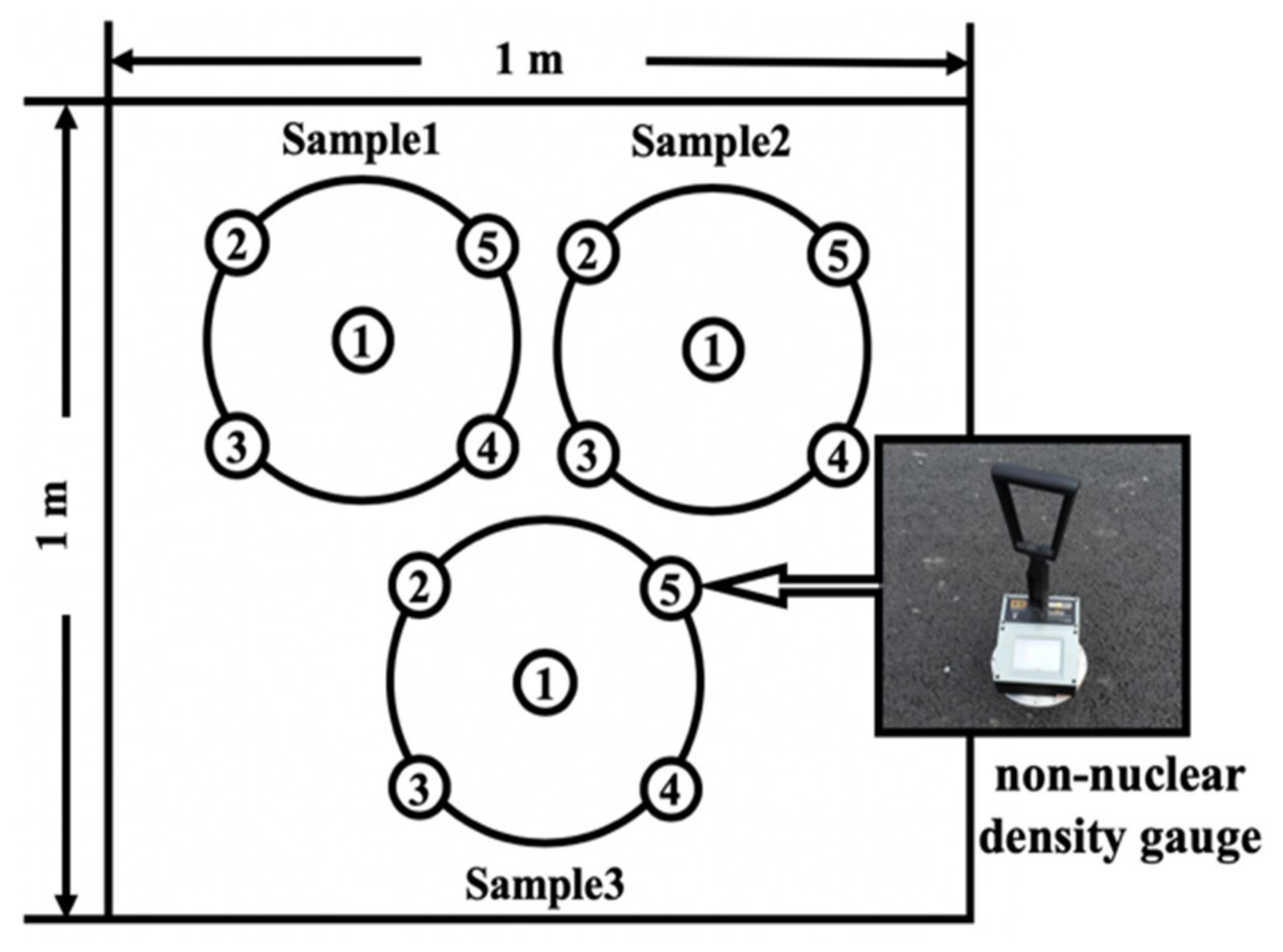
3.4. Calculation Methods of Density

For the density prediction of asphalt concrete layer, the four prediction models chosen from literature—the Birefringence, Boettcher, Linearity indicator, and Rayleigh models—are presented in Equations (7)–(10), respectively, which can calculate the bulk density of the asphalt concrete layer using the dielectric constant [20,21,22,23,24].

$$G_{mb}=\frac{\sqrt{{\epsilon }_{AC}}-1}{\frac{P_b}{G_b}\sqrt{{\epsilon }_b}+\frac{\left(1-P_b\right)}{G_{se}}\sqrt{{\epsilon }_s}-\frac{1}{G_{mm}}}$$

(7)

$$G_{mb}=\frac{\frac{{\epsilon }_{AC}-{\epsilon }_b}{3{\epsilon }_{AC}}-\frac{1-{\epsilon }_b}{1+2{\epsilon }_{AC}}}{\left(\frac{{\epsilon }_s-{\epsilon }_b}{{\epsilon }_s+2{\epsilon }_{AC}}\right)\frac{\left(1-P_b\right)}{G_{se}}-\left(\frac{1-{\epsilon }_b}{1+2{\epsilon }_{AC}}\right)\left(\frac{1}{G_{mm}}\right)}$$

(8)

$$G_{mb}=\frac{{\epsilon }_{AC}-1}{\frac{P_b}{G_b}{\epsilon }_b+\frac{\left(1-P_b\right)}{G_{se}}{\epsilon }_s-\frac{1}{G_{mm}}}$$

(9)

$$G_{mb}=\frac{\frac{{\epsilon }_{AC}-{\epsilon }_b}{{\epsilon }_{AC}+2{\epsilon }_b}-\frac{{\epsilon }_a-{\epsilon }_b}{{\epsilon }_a+2{\epsilon }_b}}{\left(\frac{{\epsilon }_s-{\epsilon }_b}{{\epsilon }_s+2{\epsilon }_b}\right)\frac{\left(1-P_b\right)}{G_{se}}-\left(\frac{{\epsilon }_a-{\epsilon }_b}{{\epsilon }_a+2{\epsilon }_b}\right)\left(\frac{1}{G_{mm}}\right)}$$

(10)

where, ε_a is the dielectric constant of air, ε_b is the dielectric constant of the bituminous binder, ε_s is the dielectric constant of aggregate, G_mb (g/cm³) is the bulk density of asphalt mixture, G_se (g/cm³) is the specific gravity of aggregate, G_mm (g/cm³) is the maximum theoretical density of asphalt mixture, P_b is the bituminous binder content. According to the results of laboratory test, ε_b = 3.5, ε_s = 7, P_b = 0.06, G_se = 2.66 g/cm³, G_mm = 2.565 g/cm³, respectively.

3.5. Calibration Method of Actual Density

The non-nuclear density gauge, PQI380, TransTech, Greenville, SC, USA, was used to detect the density of asphalt concrete base in the field test in order to confirm the appropriate calculation method from the four density calculation models. The detected data of the non-nuclear density gauge was first calibrated by the coring samples. A clean and dry area with 1 × 1 m² was selected for the calibration. Three circle areas were tested for density by the non-nuclear density gauge. Each circle area had five test points and cored a sample in the middle of the circle (Figure 4). Three coring samples in total were tested to obtain the average density in a laboratory. The results of density calibration are shown in

Table 2. Density calibration results of the non-nuclear density gauge.

Test Content	Density (g/cm3)
	Sample 1	Sample 2	Sample 3
Test Point 1	2.34	2.39	2.34
Test Point 2	2.37	2.41	2.44
Test Point 3	2.29	2.50	2.43
Test Point 4	2.37	2.51	2.54
Test Point 5	2.50	2.44	2.42
Mean of Test Points	2.37	2.45	2.44
Coring Sample	2.35	2.36	2.35

. It was found that the density tested by the coring samples was comparable to the results of the non-nuclear density gauge. The non-nuclear density detection results may be adopted to verify the estimated values by four density prediction models.

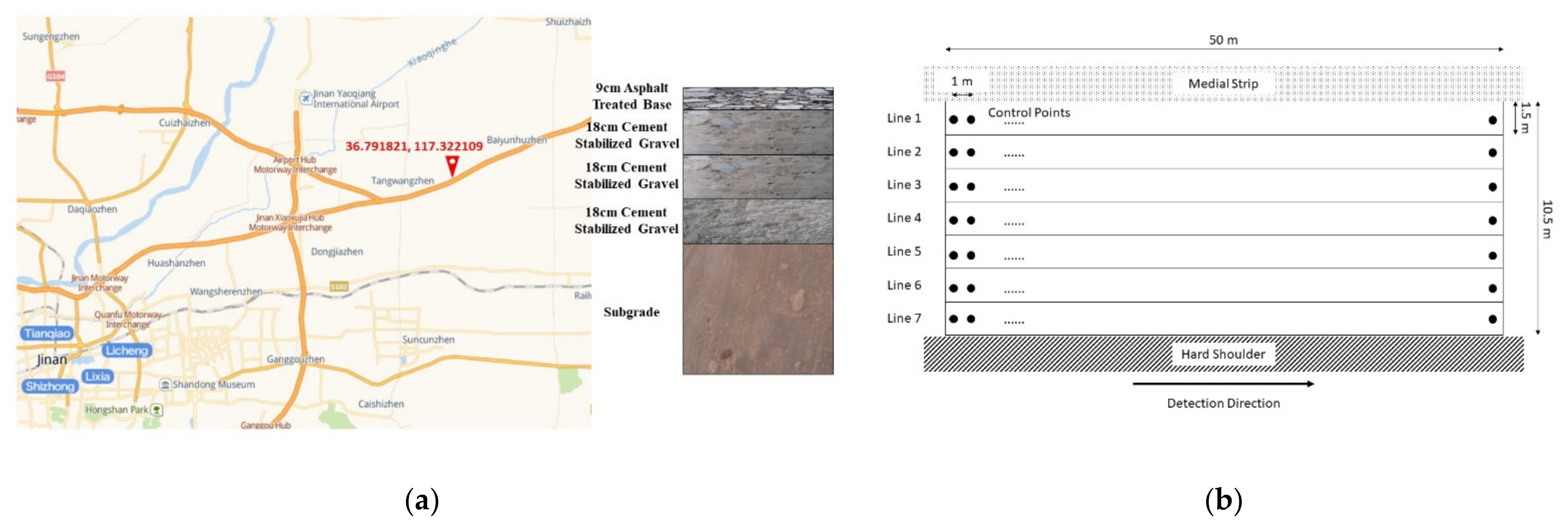
3.6. Field Test in a Newly Constructed Pavement

The field test conducted a continuous real-time GPR test on a reconstruction and extension project on the G20 highway, which was located in Jinan, Shandong Province, China, as shown in Figure 5. The asphalt concrete base of this reconstruction and extension project had already finished. The width and length of the asphalt pavement in this test were 10.5 m and 50 m, respectively. The design thickness of the asphalt concrete base was 9 cm. The asphalt mixture used in the asphalt concrete base was asphalt-treated base (ATB 25) with 70 bitumen.

In order to detect the thickness of the test area, seven parallel detection lines (Line 1 to Line 7) with a width of 1.5 m were established. Line 1 was close to the medial strip and Line 7 was located in the hard shoulder. Fifty control points of GPR detection with space between one meter per line were acquired, as shown in Figure 4. The 350 thickness values of the asphalt concrete base were calculated by Equations (4) and (5). Three coring samples of the test area were cored in order to verify the prediction thickness values.

4. Results and Discussion

4.1. Comparison of the Dielectric Constants Estimated by Different Methods

The results of the dielectric constants of the asphalt concrete layer by the Coring Method, Reflection Amplitudes Method, and The Common Mid-Point Method are shown in

Table 3. Dielectric constants of asphalt concrete calculated by three calculation methods.

Sample	Dielectric Constant			Error
	Coring Method	Reflection Amplitudes Method	Common Mid-Point Method	(εRAM − εCore)/ εCore	(εCMP − εCore)/ εCore
1	4.94	2.56	5.06	−48%	2%
2	5.67	2.66	5.48	−53%	−3%
3	4.75	3.45	4.84	−27%	2%
4	4.55	6.73	4.85	48%	7%
5	4.81	4.40	4.83	−9%	0%
Average Value	4.94	3.96	5.01	−20%	1%
Standard Deviation	0.38	1.53	0.25	-	-
Coefficient of Variation	0.08	0.39	0.05	-	-

. For the Coring method, the dielectric constant calculated ranged from 4.55 to 5.67 with an average value of 4.94. The coefficient of variation was 8%.

Based on the Reflection Amplitudes Method, the dielectric constant ranged from 2.56 to 6.73 with an average value of 3.96. And the coefficient of variation was 39%, considerably compared to the Coring Method. In general, the dielectric constant calculated by the Reflection Amplitudes Method are lower than the coring method [2]. The highest error between the dielectric constant, determined from the Coring method and the Reflection Amplitudes Method for each sample, occurred at sample 2 with −53%.

The dielectric constant calculated using the Common Mid-Point Method, ranged from 4.83 to 5.48 with an average value of 5.01. The coefficient of variation was 5%. Compared to the dielectric constant results from the Coring Method, the highest error occurred at sample 4 with 7%.

As listed in Table 2, compared to the three calculation methods, the Reflection Amplitudes Method had the highest coefficient of variation when analyzing all five points. The Coring Method and the Common Mid-Point Method had similar average values and coefficient of variation for calculating dielectric constants of the asphalt concrete layer. The Coring Method was the most accurate way because it had a real parameter from the cores. However, the Coring Method was also inefficient with coring in the test area.

According to the results of calculation, the Common Mid-Point Method showed reasonable agreement with cores and acquired dielectric constants of the asphalt concrete layer in all the areas. In this study, the Common Mid-Point Method was then recommended.

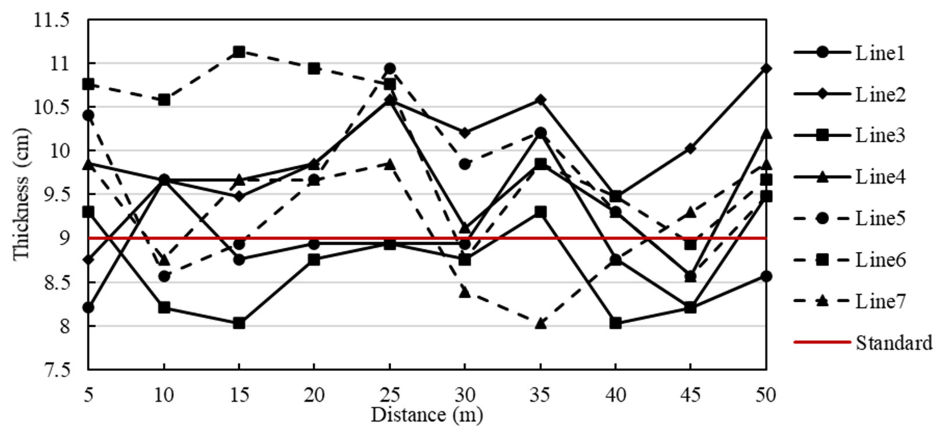
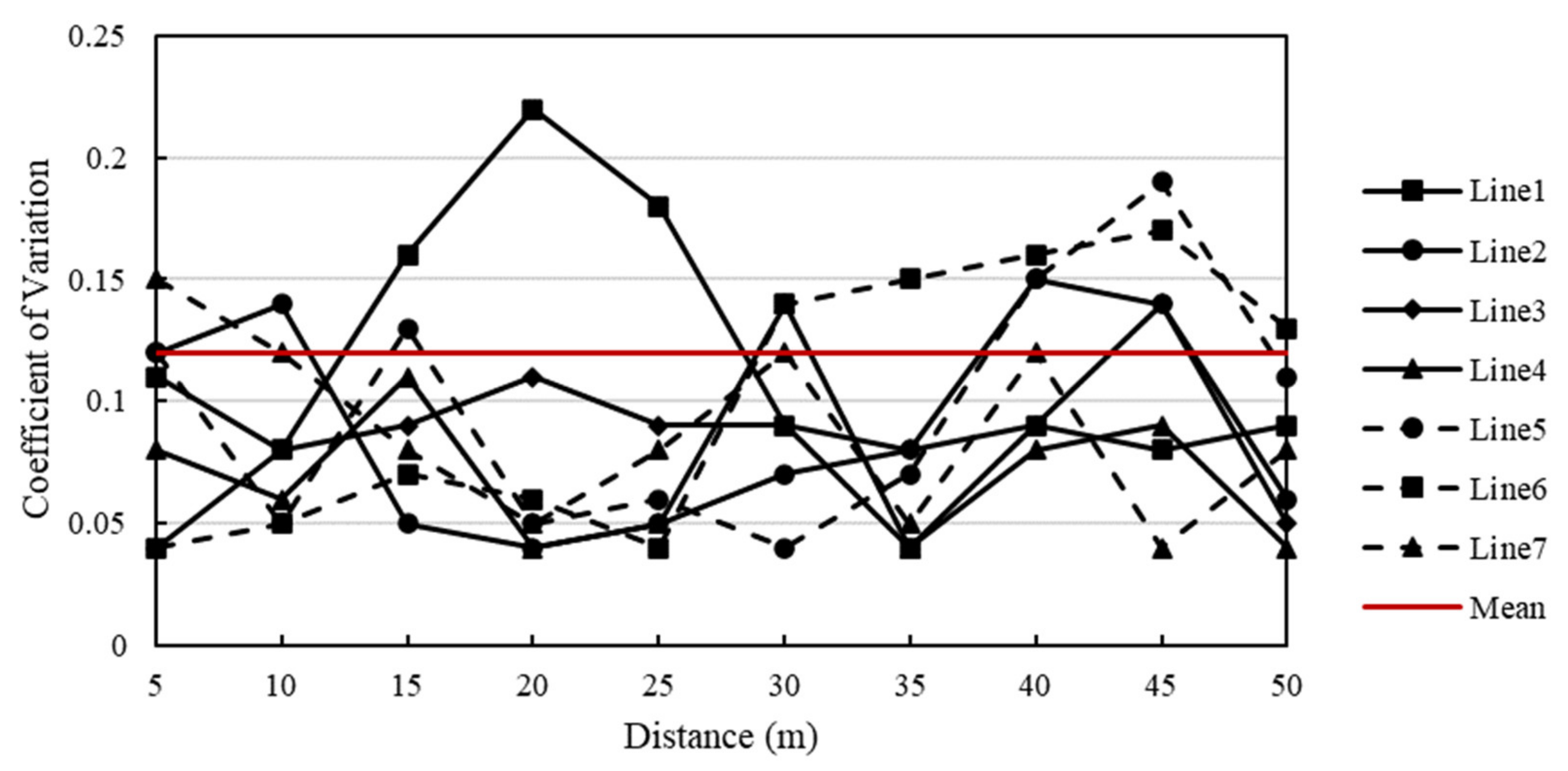
4.2. Assessment of Thickness Homogeneity

In terms of the dielectric constants calculated by the Common Mid-Point Method, the thickness distribution of the asphalt concrete base in the tested area is shown in Figure 6. In total, there were 350 tested points, where 7 intervals with 1.5 m along the width (line 1, line 2, line 3, line 4, line 5, line 6 and line 7) and 50 intervals with 1 m along the 50 m long pavement were chosen equally, respectively. It was found that the thickness of 88 tested points of thickness was less than 9 cm. Its proportion of total test area was 25%. The thickness correction factor and the mean value of the corrected thickness are shown in

Table 4. Thickness correction factor.

Test Contents	Sample 1	Sample 2	Sample 3
Coring Thickness	11.2 cm	9.2 cm	10.6 cm
Calculated Thickness	12.0 cm	10.0 cm	12.0 cm
Coring/Calculated	0.933	0.920	0.883
Correction Factor	Mean = 0.912

and

Table 5. Mean value of corrected thickness.

Test Contents	Thickness (cm)
	Line 1	Line 2	Line 3	Line 4	Line 5	Line 6	Line 7
Mean	8.92	9.96	8.7	9.67	9.59	10.09	9.21
Standard Deviation	1.15	1.02	0.93	0.87	1.18	1.27	1.03
Coefficient of Variation	0.13	0.10	0.11	0.09	0.12	0.13	0.11
All Area Mean	9.45
All Area Standard Deviation	1.17
All Area Coefficient of Variation	0.12

.

In Table 5, the maximum mean value of thickness was Line 6 and the minimum one was Line 3. The mean value, the standard deviation, and the coefficient of variation of thickness in all the test areas were 9.45, 1.17, and 0.12 cm, respectively. The results showed that the thinner areas were located in Line 1 and Line 3, which was close to the edge of the pavement and the middle of the asphalt paver.

In order to assess the thickness homogeneity of the asphalt concrete base more qualitatively, the test area (Line 1 to Line 7) was divided into 70 units, and each unit was 1.5 m in width and 5 m in length, shown in Figure 5b. The mean thickness values of every area were calculated and are shown in Figure 7. The red line was the design thickness of the asphalt concrete base. The results of all lines showed thickness variation, and the thickness of Line 3, Line 1, and Line 7 were lower than that of the designed thickness value. The Line 5 thickness had the highest variation. The thickness of the asphalt concrete base showed that the thinner area was close to the edge of the pavement and the middle section of the asphalt paver.

Figure 8 is the thickness coefficient of variation of the test area. The mean coefficient of variation in Line 4 was 0.073 and showed the best thickness homogeneity.

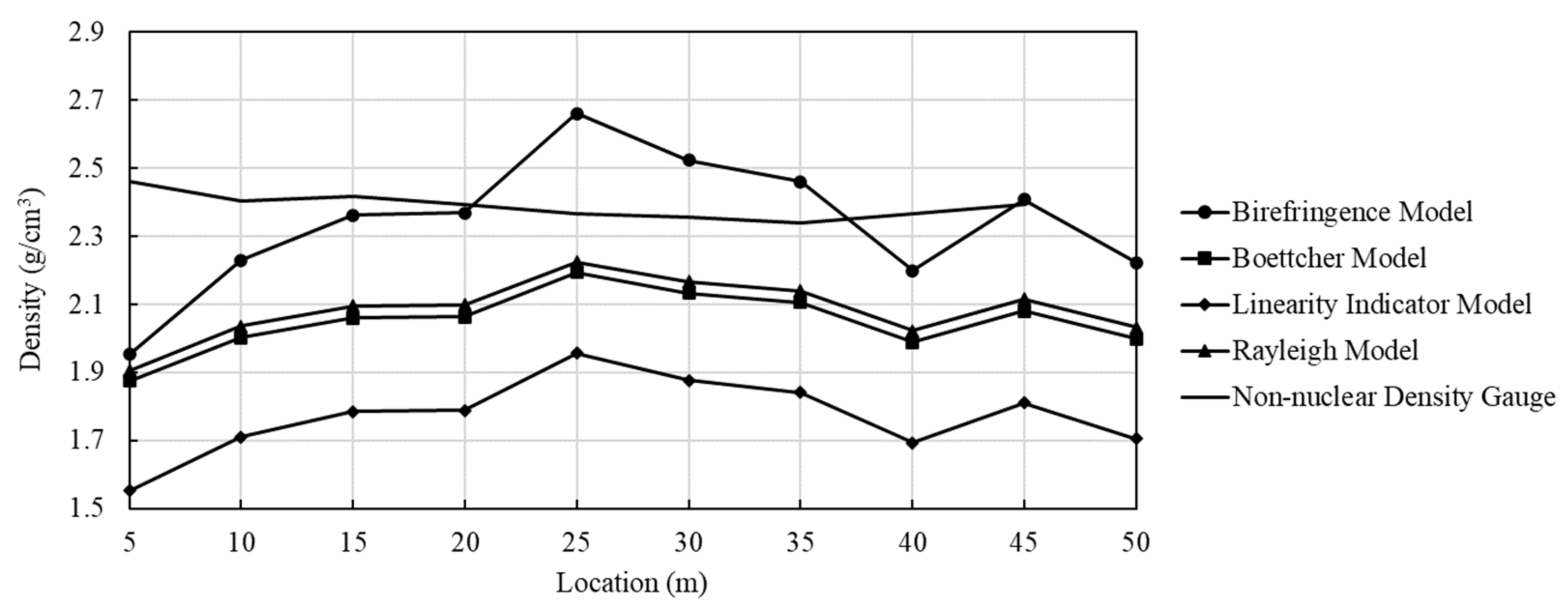
4.3. Assessment of Density Homogeneity

In terms of the four density prediction models, the predicted bulk densities of asphalt concrete base in the field test are shown in

Table 6. Density of the asphalt concrete layer in Line 4 calculated by the four prediction models.

Location	Dielectric Constant	Birefringence Model	Boettcher Model	Linearity Indicator Model	Rayleigh Model
		Bulk Density (g/cm3)
5 m	4.54	1.95	1.88	1.55	1.91
10 m	4.90	2.23	2.00	1.71	2.04
15 m	5.07	2.36	2.06	1.79	2.10
20 m	5.08	2.37	2.06	1.79	2.10
25 m	5.46	2.66	2.19	1.96	2.23
30 m	5.28	2.52	2.13	1.88	2.17
35 m	5.20	2.46	2.11	1.84	2.14
40 m	4.86	2.20	1.99	1.69	2.02
45 m	5.13	2.41	2.08	1.81	2.12
50 m	4.89	2.22	2.00	1.71	2.03

. In order to not affect the construction period, Line 4 was selected and used to predict the density. The predicted density compared with the measurement density by non-nuclear density gauge is shown in Figure 9. The correlation coefficient of prediction density with measurement density was calculated and is shown in

Table 7. Correlation coefficient of the predicted density with the measured density.

Prediction Model	Birefringence Model	Boettcher Model	Linearity Indicator Model	Rayleigh Model
Correlation Coefficient	−0.712	−0.714	−0.713	−0.719

. The predicted density of the four models had a similar correlation coefficient with the measured density. The density by the Birefringence model had an obvious volatility and the difference value between maximum density and minimum density was 0.71. The results of the Linearity Indicator model deviated highly with the measured density than the other models. The Boettcher model and the Rayleigh model had similar results, but the density predicted by the Rayleigh model closed to the measured density.

The Rayleigh model presented the highest correlation coefficient when compared with the results from the four prediction models. This model had the potential way to calculate and corrected the density by GPR data. The Rayleigh model was then used to predict the density and the correction factor. The correction factor was the ratio of density obtained by the non-nuclear density gauge and the Rayleigh model (G Non-nuclear/G Rayleigh). Therefore, the continuous prediction of density and the correction factor compared to the non-nuclear density gauge results in the test field are shown in

Table 8. Density correction factor of the Rayleigh model.

Location	Rayleigh Model	Non-Nuclear Density Gauge	Correction Factor (G Non-Nuclear/G Rayleigh)	Mean
5 m	1.91	2.46	1.29	1.15
10 m	2.04	2.41	1.18
15 m	2.10	2.42	1.15
20 m	2.10	2.39	1.14
25 m	2.22	2.37	1.06
30 m	2.17	2.36	1.09
35 m	2.14	2.34	1.09
40 m	2.02	2.37	1.17
45 m	2.12	2.39	1.13
50 m	2.03	2.39	1.17

. The predicted density results had an average correction factor of 1.15, compared to the measured density from the non-nuclear density gauge. With this correction factor, the GPR data and Rayleigh model was able to calculate the accurate density of asphalt pavement without coring or non-nuclear density gauge. In the application of practical road projects, this method could save a lot of testing time and improve the efficiency of quality control.

The Rayleigh model was then used to predict the density of the parallel test lines in the tested area. The density distributions of the asphalt concrete base in the seven tested lines are presented in Figure 10. Line 1, Line 6, and Line 7 had relatively low density in the asphalt concrete base. These results indicate that the edge of asphalt concrete base showed segregation of the asphalt mixture. Insufficient compaction of the asphalt mixture was one of the reasons for low-density distribution. According to the results of density detection by the GPR and Rayleigh model, the construction technology of paving and compaction could be improved.

5. Conclusions

Although the air-launched 3D GPR is nondestructive, time-saving, and less labor-intensive to assess density and thickness, it can only provide indirect measurement data under testing area conditions and strongly depends on the explanations by prediction models. This study focused on the adaptability and accuracy of different prediction models to calculate the dielectric constant, thickness, and density of an asphalt concrete base. By choosing proper calculation methods, the thickness and density of this layer were predicted, and homogeneity was assessed. The main findings were given below:

(1)

The Common Mid-Point Method, using the air-launched bowknot monopole antennae matrix, had a satisfactory performance in determination of the dielectric constant of the asphalt concrete base and presented an error of 1%, when compared with the calculated dielectric constant from cores. The results indicated potential of the Common Mid-Point Method to be adopted for providing reliable estimation results on the dielectric constant of an asphalt concrete layer and obtaining accurate calculated thickness.

(2)

In terms of GPR and the Common Mid-Point Method, thickness homogeneity assessment on the tested filed found that the thickness of an asphalt concrete base showed the thin area to be close to the edge of the pavement and the middle section of the asphalt concrete base.

(3)

Among the Birefringence, Boettcher, Linearity indicator, and Rayleigh models, the Rayleigh model was suggested to predict density, and the predicted density exhibited a good correlation coefficient with the measured density. The results of the Rayleigh model presented an average correction factor of 1.15, when compared to the density from the non-nuclear density gauge.

However, the Common Mid-Point Method was only able to detect a line area and the detection dielectric constants were a representative value of small areas. The variation of dielectric constants in the small area should be considered. In this study, only asphalt pavement layers were researched. The applications of GPR also included cement concrete pavements.

References

1. Wang, S.Q.; Zhao, S.; Al-Qadi, I. Continuous real-time monitoring of flexible pavement layer density and thickness using ground penetrating radar. NDT E Int. 2018, 100, 48–54. [Google Scholar] [CrossRef]
2. Zhao, S.; Al-Qadi, I. Development of regularization methods on simulated ground-penetrating radar signals to predict thin asphalt overlay thickness. Signal Process. 2017, 132, 261–271. [Google Scholar] [CrossRef]
3. Leng, Z.; Al-Qadi, I.; Shangguan, P.C.; Son, S. Field application of Ground-Penetrating Radar for measurement of asphalt mixture density case study of Illinois Route 72 overlay. Transp. Res. Rec. J. Transp. Res. Board 2012, 2304, 133–141. [Google Scholar] [CrossRef]
4. Al-Qadi, I.; Lahouar, S. Measuring layer thicknesses with GPR-theory to practice. Constr. Build. Mater. 2005, 19, 763–772. [Google Scholar] [CrossRef]
5. Loizos, A.; Plati, C. Accuracy of pavement thicknesses estimation using different ground penetrating radar analysis approaches. NDT E Int. 2007, 40, 147–157. [Google Scholar] [CrossRef]
6. Aleksey, K.; Aleksandra, V.; Evgeniy, V.T.; Anderson, N.L.; Sneed, L.H. Utilization of air-launched ground penetrating radar (GPR) for pavement condition assessment. Constr. Build. Mater. 2017, 141, 130–139. [Google Scholar]
7. Wallace, W.L.; Xavier, D.; Peter, A. A review of Ground Penetrating Radar application in civil engineering: A 30-year journey from Locating and Testing to Imaging and Diagnosis. NDT E Int. 2018, 96, 58–78. [Google Scholar]
8. Mezgeen, R.; Vega, P.; Mercedes, S.; Jorge, C.; Pais, F.; Caio, S. An experimental and numerical approach to combine Ground Penetrating Radar and computational modelling for the identification of early cracking in cement concrete pavements. NDT E Int. 2020, 115, 102293. [Google Scholar]
9. Mercedes, S.; Susana, L.; Belen, R.; Henrique, L. Non-destructive testing for the analysis of moisture in the masonry arch bridge of Lubians (Spain). Struct. Control Health Monit. 2013, 20, 1366–1376. [Google Scholar]
10. Saarenketo, T.; Scullion, T. Road evaluation with ground penetrating radar. J. App. Geophys. 2000, 43, 119–138. [Google Scholar] [CrossRef]
11. Al-Qadi, I.; Leng, Z.; Lahouar, S.; Baek, J. In-place hot-mix asphalt density estimation using ground-penetrating radar. Transp. Res. Rec. J. Transp. Res. Board 2010, 2152, 19–27. [Google Scholar] [CrossRef] [Green Version]
12. Shangguan, P.C.; Al-Qadi, I.; Coenen, A.; Zhao, S. Algorithm development for the application of ground-penetrating radar on asphalt pavement compaction monitoring. Int. J. Pavement Eng. 2016, 17, 189–200. [Google Scholar] [CrossRef]
13. Zhao, S.; Shangguan, P.C.; Al-Qadi, I. Application of regularized deconvolution technique for predicting pavement thin layer thicknesses from ground penetrating radar data. NDT E Int. 2015, 73, 1–7. [Google Scholar] [CrossRef]
14. Zhao, S.; Al-Qadi, I. Development of an analytic approach utilizing the extended common midpoint method to estimate asphalt pavement thickness with 3-D ground-penetrating radar. NDT E Int. 2016, 78, 29–36. [Google Scholar] [CrossRef]
15. Plati, C.; Loizos, A. Using ground-penetrating radar for assessing the structural needs of asphalt pavement. Nondestr. Test. Eval. 2012, 27, 273–284. [Google Scholar] [CrossRef]
16. Maser, K.R.; Scullion, T. Automated pavement subsurface profiling using radar: Case studies of four experimental field sites. Transp. Res. Rec. J. Transp. Res. Board 1992, 1344, 148–154. [Google Scholar]
17. Poikajarvi, J.; Peisa, K.; Herronen, T.; Aursand, P.O.; Maijala, P.; Narbro, A. GPR in road investigations-equipment tests and quality assurance of new asphalt pavement. Nondestr. Test. Eval. 2012, 27, 293–303. [Google Scholar] [CrossRef]
18. Goel, A.; Das, A. Nondestructive testing of asphalt pavements for structural condition evaluation: A state of the art. Nondestr. Test. Eval. 2008, 23, 121–140. [Google Scholar] [CrossRef]
19. Spagnolini, U. Permittivity measurements of multilayered media with monostatic pulse radar. IEEE Trans. Geosci. Remote 1997, 35, 454–463. [Google Scholar] [CrossRef] [Green Version]
20. Zhao, S.; Al-Qadi, I. Algorithm development for real-time thin asphalt concrete overlay compaction monitoring using ground-penetrating radar. NDT E Int. 2019, 104, 114–123. [Google Scholar] [CrossRef]
21. Plati, C.; Georgouli, K.; Cliatt, B.; Loizos, A. Incorporation of GPR data into genetic algorithms for assessing recycled pavements. Constr. Build. Mater. 2017, 154, 1263–1271. [Google Scholar] [CrossRef]
22. Eskelinen, P.; Pellinen, T. Comparison of different radar technologies and frequencies for road pavement evaluation. Constr. Build. Mater. 2018, 164, 888–898. [Google Scholar] [CrossRef]
23. Tosti, F.; Ciampoli, L.B.; D’Amico, F.; Alani, A.M.; Benedetto, A. An experimental-based model for the assessment of the mechanical properties of road pavements using ground-penetrating radar. Constr. Build. Mater. 2018, 165, 966–974. [Google Scholar] [CrossRef]
24. Araujo, S.; Beaucamp, B.; Delbreilh, L.; Dargent, É.; Fauchard, C. Compactness/density assessment of newly-paved highway containing recycled asphalt pavement by means of non-nuclear method. Constr. Build. Mater. 2017, 154, 1151–1163. [Google Scholar] [CrossRef]
25. Yao, K.; Chen, Q.; Xiao, H.; Liu, Y.; Lee, F.H. Small-strain shear modulus of cement-treated marine clay. J. Mater. Civ. Eng. 2020, 32, 04020114. [Google Scholar] [CrossRef]
26. Marecos, V.; Fontul, S.; Solla, M.; de Lurdes Antunes, M. Evaluation of the feasibility of Common Mid-Point approach for air-coupled GPR applied to road pavement assessment. Measurement 2018, 128, 295–305. [Google Scholar] [CrossRef]
27. Hu, J.H.; Vennapusa, P.; White, D.J.; Beresnev, I. Pavement thickness and stabilized foundation layer assessment using ground-coupled GPR. Nondestr. Test. Eval. 2016, 31, 267–287. [Google Scholar] [CrossRef]
28. Marecos, V.; Fontul, S.; Antunes, M.; Solla, M. Evaluation of a highway pavement using non-destructive tests Falling Weight Deflectometer and Ground Penetrating Radar. Constr. Build. Mater. 2017, 154, 1164–1172. [Google Scholar] [CrossRef]
29. Dong, Z.H.; Ye, S.B.; Gao, Y.Z.; Fang, G.; Zhang, X.; Xue, Z.; Zhang, T. Rapid detection methods for asphalt pavement thicknesses and defects by a vehicle-mounted Ground Penetrating Radar (GPR) system. Sensors 2016, 16, 2067. [Google Scholar] [CrossRef] [Green Version]
30. Kassem, E.; Chowdhury, A.; Scullion, T.; Masad, E. Application of ground-penetrating radar in measuring the density of asphalt pavements and its relationship to mechanical properties. Int. J. Pavement Eng. 2016, 17, 503–516. [Google Scholar] [CrossRef]
Figure 1. GPR system.
Coatings 11 01398 g001
Figure 2. The amplitude of the GPR test. (a) Reflection on the surface; (b) Reflection on a metal plate.
Coatings 11 01398 g002
Figure 3. Schematic diagram of CMP.
Coatings 11 01398 g003
Figure 4. Schematic of density calibration in the field test.
Coatings 11 01398 g004
Figure 5. Location and pavement structure of the field test. (a) Location and structure; (b) Test area.
Coatings 11 01398 g005
Figure 6. Thickness distribution of the asphalt concrete base in the tested area.
Coatings 11 01398 g006
Figure 7. Mean values of thickness in 70 evaluated areas.
Coatings 11 01398 g007
Figure 8. Thickness coefficient of variation in 70 evaluated areas.
Coatings 11 01398 g008
Figure 9. Comparison of the predicted density by the four prediction models and the measured density by the non-nuclear density gauge.
Coatings 11 01398 g009
Figure 10. Density distribution of the tested area.
Coatings 11 01398 g010