Heat Transfer Impacts on Maxwell Nanofluid Flow over a Vertical Moving Surface with MHD Using Stochastic Numerical Technique via Artificial Neural Networks

Abstract

The technique of Levenberg–Marquardt back propagation with neural networks (TLMB-NN) was used in this research article to investigate the heat transfer of Maxwell base fluid flow of nanomaterials (HTM-BFN) with MHD over vertical moving surfaces. In this study, the effects of thermal energy, concentration, and Brownian motion are also employed. Moreover, the impacts of a heat-absorbing fluid with viscous dissipation and radiation have been explored. To simplify the governing equations from a stiff to a simple system of non-linear ODEs, we exploited the efficacy of suitable similarity transformation mechanism. Through applicability of state-of-the-art Adams numerical technique, a set of data for suggested (TLMB-NN) is generated for several situations (scenarios) by changing parameters, such as the Thermophoresis factor N_t, Hartmann number M, Eckert number E_c, concentration Grashoff parameter G_c, Prandtl number P_r, Lewis number Le, thermal Grashof number G_T, and Brownian motion factor N_b. The estimate solution of different instances has validated using the (TLMB-NN) training, testing, and validation method, and the recommended model was compared for excellence. Following that, regression analysis, mean square error, and histogram explorations are used to validate the suggested (TLMB-NN). The proposed technique is distinguished based on the proximity of the proposed and reference findings, with an accuracy level ranging from 10⁻⁹ to 10⁻¹⁰.

1. Introduction

Artificial Neural Networks (ANNs) are a groundbreaking new AI (artificial intelligence) technique. ANNs can grow in a variety of modes, depending on the data that flows through the network throughout the learning process, whether internally or externally. To increase the performance of a Multilayer Perceptron (MLP) network, an artificial neural network uses the Back Propagation (BP) method to undertake simultaneous training. It is the most widely used, effective, and simple-to-learn paradigm for complex multi-layered networks. Paul Werbos, who created the back propagation method in 1974, was the first to do so, while Rumelhart and Parker were the first to revive it (see ref. [1]). The Levenberg–Marquardt methodology/algorithm (LMA) is an innovative convergent reliability technique for artificial neural networks (ANNs) that provides a numerical solution to a wide range of fluid flow issues. Several researchers have recently used this method to examine mass and heat-transmission features, along with non-Newtonian fluid flow systems. Raja, M.A.Z et al. [2] suggest neural networks approach with backpropagation to analysis the 3D hall current of Cattaneo–Christov heat flux model relating biconvection nanofluidic flow with Darcy–Forchheimer law influence. Shoaib et al. [3] investigated the generation of entropy under the impact of MHD and thermal radiation using the proficiency of neural networks. Khan et al. [4] used a Backpropagated neural network optimized with Levenberg-Marquardt scheme (BNN-LMS) to investigate heat transport between two permeable parallel plates of steady Nano fluids applying Thermophoresis and Brownian impacts. To explain the third-order nonlinear scheme of Emden–Fowler paradigm, Sabir et al. [5] examined computational intelligence methodology employing Levenberg–Marquardt backpropagation neural networks. Using TLMB-NN based computational intelligence, Uddin et al. [6] showed how to combine magnetic and radiation effects to comprehend the investigation of Maxwell Nano liquid thin film stream across a stretchy and spinning disc.

As the efficiency of appliances and thermal schemes is associated to heat-transfer amounts, engineers and researchers have engaged on the issue of poor thermal conductivity and the subsequent weak heat-transmission factors proposed by convectional fluids, for example, water, glycol, ethylene oil, etc. Choi [7,8] exposed and demonstrated that the upmost-needed greater conducting liquid for improving the cooling scheme in maximum engineering and industrial appliances can be accomplished by combining nanometer-sized particles, for example, caused by carbides, carbon nanotubes, metals and oxides, etc., with conventional heat-transportation fluids. Various investigators have drawn to the fascinating and expressive evaluation of Nano fluids due to the auspicious purposes for example solid-state lighting, nuclear reactors, electronic appliances, safer surgery, and cancer therapy that might enhance heat-transfer competence for an improved cooling method Nayak et al. [9]. Nano fluid characteristics like as viscosity and thermal conductivity have a significant impact on heat-transmission rates, according to Sheikholeslami et al. [10]. As a result, the utilization of ultra-fine solid particles in fluids has affected significantly the improvement of heat-transmission execution. According to Nima et al. [11], such a variety develops in a more conductive heat-transfer liquid, which has uses in electronics, transportation sectors, pharmaceutical sectors, biomedicine, atomic reactors, and power manufacture, etc. According to Eastman et al. [12], the heat-absorption capacity of Nano fluids is significantly higher than that of conventional fluids, with thermal conductivity rising equal to 40% dependent on the size, shape, and thermal properties of solid nanomaterials. Various thermophysical characteristics of Nano fluids have been investigated by many researchers in relation to these important applications, as seen in references [13,14] and their referred references. Concerning the flows in porous medium, the literature review displays that countless explorations of curiosity have been done. In fluid-saturated porous media the convective flow has been mainly inspired by its significant role in many natural and industrial problems in recent studies of interest. The heat-transfer study of incorporating the effects of porosity is significant. Keeping in view the porosity effects, Maleki et al. [15] reported the analysis of nanoliquid over a porous radiative plate. In porous medium for the problem of steady flow over a rotating disk, Mohimanian and Rashidi [16], used the HAM, involving two auxiliary parameters for the analytic estimated solution.

A lot of consideration has been given in recent years for the study of boundary layer flow of magneto hydrodynamics (MHD) and heat transfer owing to its uses in engineering and manufacturing. Pavlov et al. [17] investigated MHD boundary layer flow of an electrically conducting fluid in the existence of a constant transverse magnetic field, and Chakrabarti and Gupta et al. [18] expanded the study to include heat transmission and hydro magnetic flow. Several researchers have approved the exploration of the MHD influence on Nano fluids. Shagaiya Daniel et al. [19] studied that optical grafting, metal casting, crystal growth, metallurgical process, tunable optical fiber filters, the polymer industry, liquid metal cooling blankets for fusion reactors, and including the stretching of plastic sheets are just a few of the many uses of MHD. In a magnetic area, MHD is concerned with the movement of an electrically behaving fluid, which has the potential to regulate the system’s flow and heat transmission.

The magnetic field, when applied to nanofluids, magnetizes the flow, creating magneto–hydrodynamic flow. The MHD flow under the influence of thermal radiation has always been an interesting area for the researcher. The MHD flow studied the involvement between the electrically conductive fluid and magnetic field. Thermal radiation affects the concentration of molecules and enhances the temperature by increasing energy and molecular movement.

The primitive studies showing anomalous improvements in nanofluid thermal properties over those of the base fluid, specifically the heat-transfer coefficient, have been largely discredited. Thermophysical properties of nanofluid are not designated via classical theories due to their conventional suspensions. Measurements of the thermophysical properties of nanofluids impart only integral information about their transport processes and, as a rule, do not clarify the mechanisms of these processes. The mechanisms of transport processes were studied using the molecular dynamics method. Furthermore, the densities of the nanoparticles material play an important role in the improvement of the thermal conductivities of the nanoparticles. Moreover, the heat-transfer coefficient of the nanoparticles is of great importance due to concentration of the particles involved the fluid. It can accelerate the heat-transfer system in the nanofluids as compared to base fluid [20,21,22].

The esteem of the Maxwell fluid, which is appropriate to the rate of those kinds of fluids, is owing to its simplicity and ability to anticipate stress relaxation, as well as its tremendous behaviour in engineering and trade activity, particularly in the polymer areas. The research of [23,24,25] provides appropriate information about Maxwell fluid. Various researchers have been interested in the flow issues with a stable or continually moving flat plate since the past century, because it has numerous technical applications in disciplines such as aerodynamics, naval architecture, and so on. Applying boundary layer theory, Sakiadis [26] investigated the flow through a continually moving flat plate. Merkin [27] explored free stream flow across a vertical flat surface, including the impacts of buoyancy forces. Wilks [28] explained above a fixed flat upright surface the constant free stream flows in the semi-infinite field. Ghalambaz et al. [29] analyzed the mixed convection boundary layer flow and heat transfer over a vertical plate embedded in a porous medium filled with a suspension of nano-encapsulated phase change materials. Similarly, S.A.M. Mehryan et al. [30] explained the natural convection flow of a suspension containing nano-encapsulated phase change particles in an eccentric annulus. Because of buoyancy forces, the flow develops, and a continuous heat flux is delivered to the stationary upright plate. Bachok et al. [31] explained the heat-transmission research of a comparable free stream flow owing to a sliding flat permeable plate. By using boundary layer estimation, Sadeghy et al. [32] analyzed the Maxwell fluid flow across a moving flat plate. Damseh [33] reported the flow of viscoelastic fluid across an infinitely porous perpendicular flat plate with first-order chemical effects. Nadeem et al. [34] explained the MHD Maxwell Nano fluid flow across a flat plate in motion. With boundary coating estimations, Zhao et al. [35] addressed the unsteady naturally convected Maxwell fluid flow through a perpendicular uniform surface. Utilizing boundary layer theory, Bhatti et al. [36] investigated MHD Nano fluid flow through a porous stretched cylinder, as well as the impacts of heat radiation and chemical reactivity. With boundary coating flow assumptions, Bachok et al. [37] explained the Nano fluid flow owing to a uniform moving surface. Employing boundary layer theory, we show the flow of magneto hydrodynamics Maxwell Nano fluid across an upright moving uniform permeable plate with impacts of heat and concentration buoyancy. With radiation and viscous dissipation results, heat-absorbing fluids have deliberated.

Because finding an accurate solution to a problem analytically might be challenging, the investigator uses a combination of numerical and semi-numerical approaches to solve the problem. The Method of Spectral Relaxation [38], HPM [39], Keller Box Method [40], Galerkin finite element method [41], and many others are examples of approaches. All of the mentioned literature on Nano fluid flow for many fluidic systems was formed exploiting and utilizing various numerical and semi-numerical methodologies; however, AI-based numerical computing paradigms are critical to using HTM-BFN model, i.e., to investigate the heat transmission of Maxwell base fluid flow of nanomaterials with MHD above perpendicular moving surfaces. Evolutionary estimation approaches are used in stochastic numerical calculating solvers connected to neural networks to get the solutions/outcomes of differential equations for linear and non-linear, exhibiting different measurements of various circumstances. The engagement of these approaches comprises COVID-19 Models [42,43], mosquito dispersal model [44], atomic physics [45], magneto hydrodynamics [46,47], Emden Fowler system [48,49], thermodynamics [50], nonlinear corneal shape model [51], nanotechnology [52], and flow model of non-linear unipolar electro hydrodynamic pump [53]. All of these inspiring features boost investigators to use a reliable and perfect AI algorithm-based numerical computational model for numerical exploration of the Magneto-hydrodynamic Nano-fluid mathematical paradigm by using numerical and graphical analyses to examine the influence of all variations or physical gauges on velocity, concentration, and temperature profiles. MATLAB and Mathematica tools are used to simulate numerical behavior.

The following are the prominent aspects of the proposed design-computing methodology:

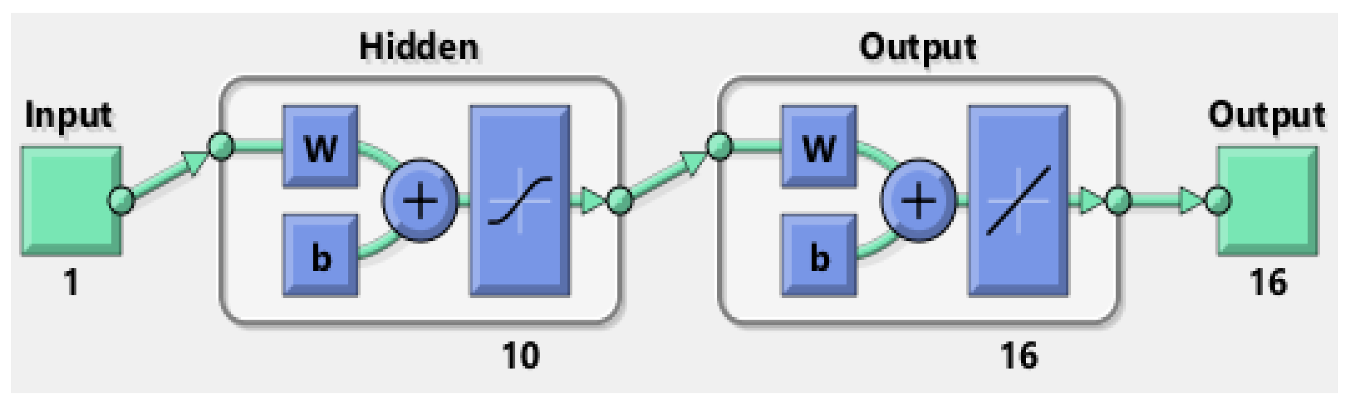
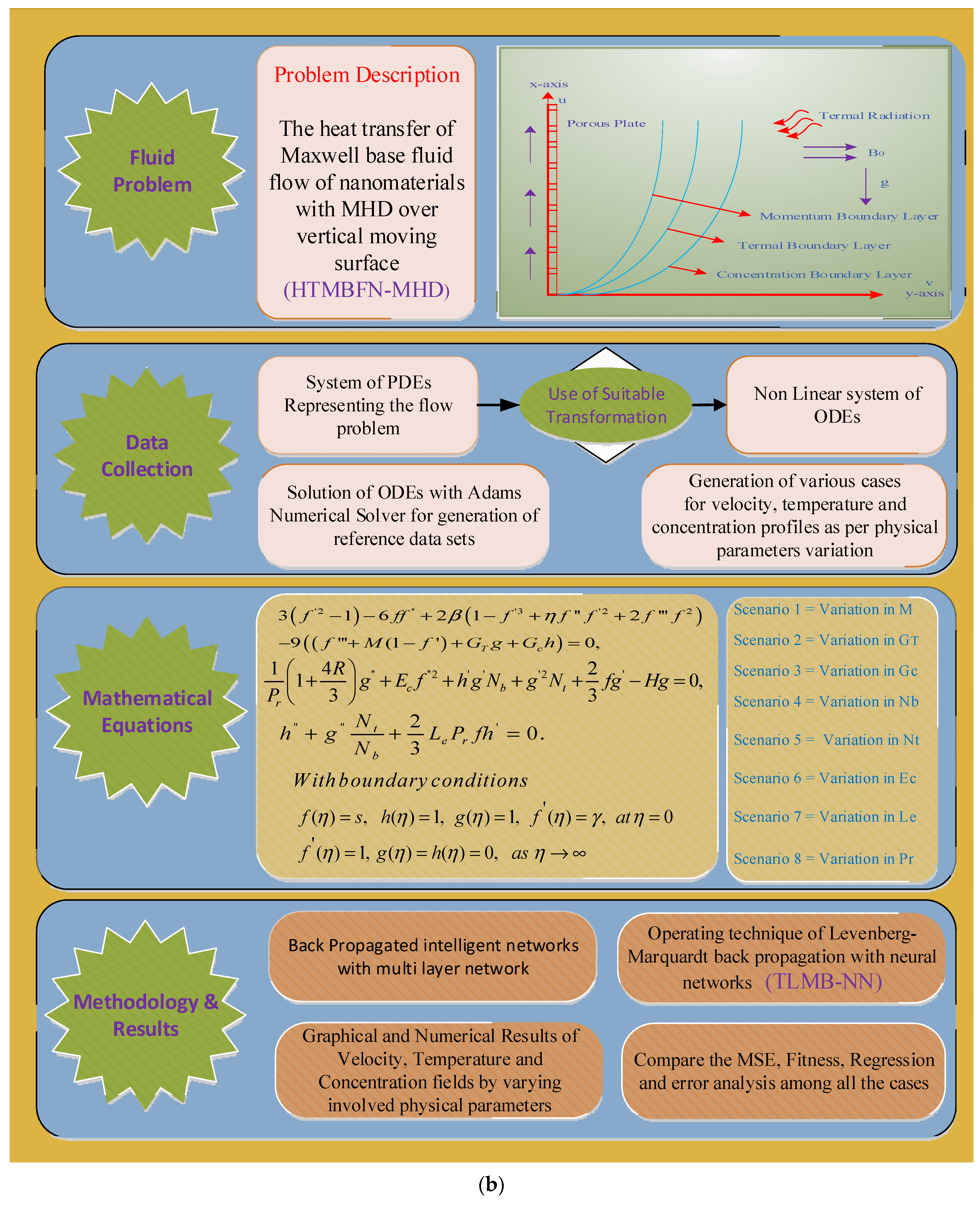
• A new AI-based intelligent computing methodology via Levenberg–Marquardt back propagation with neural networks (TLMB-NN) is used to viably explore the solution dynamics for the heat transfer of Maxwell base fluid flow of nanomaterials (HTM-BFN) with MHD;
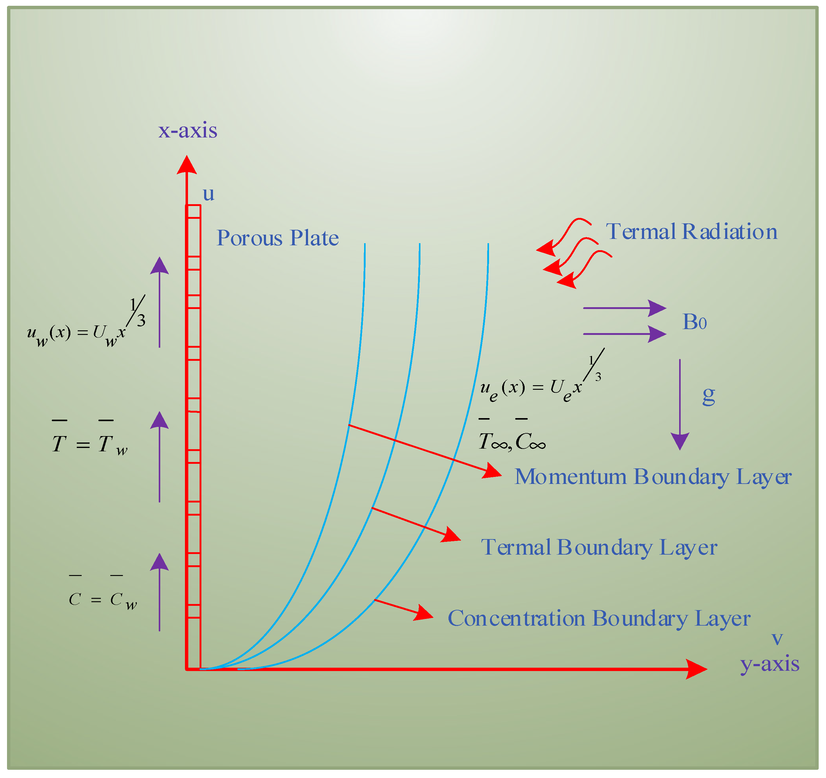
• By providing the required equivalent modification, the mathematical modeling of the novel design HTM-BFN in expressions of PDEs has transformed to similar non-linear ODEs;
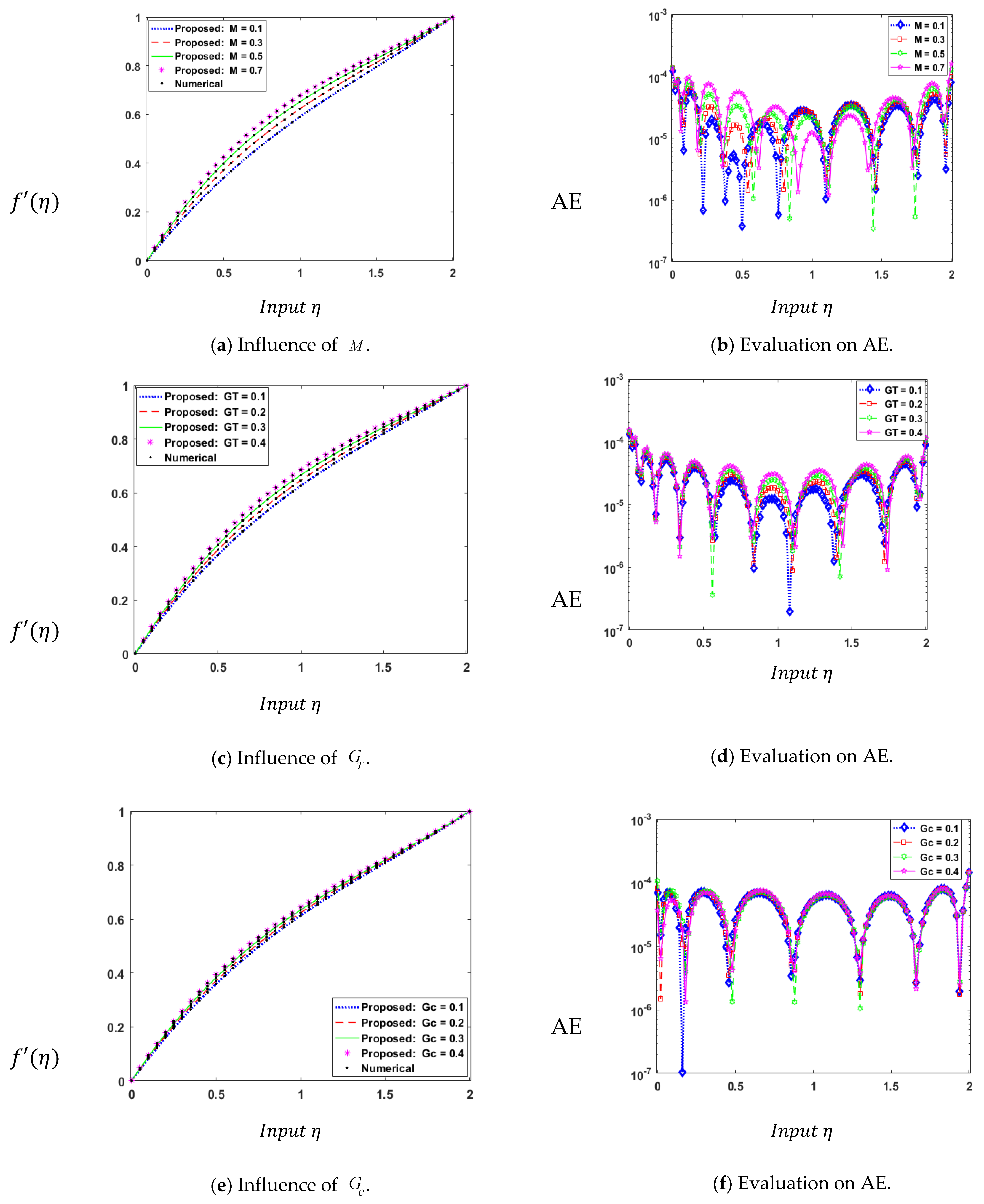
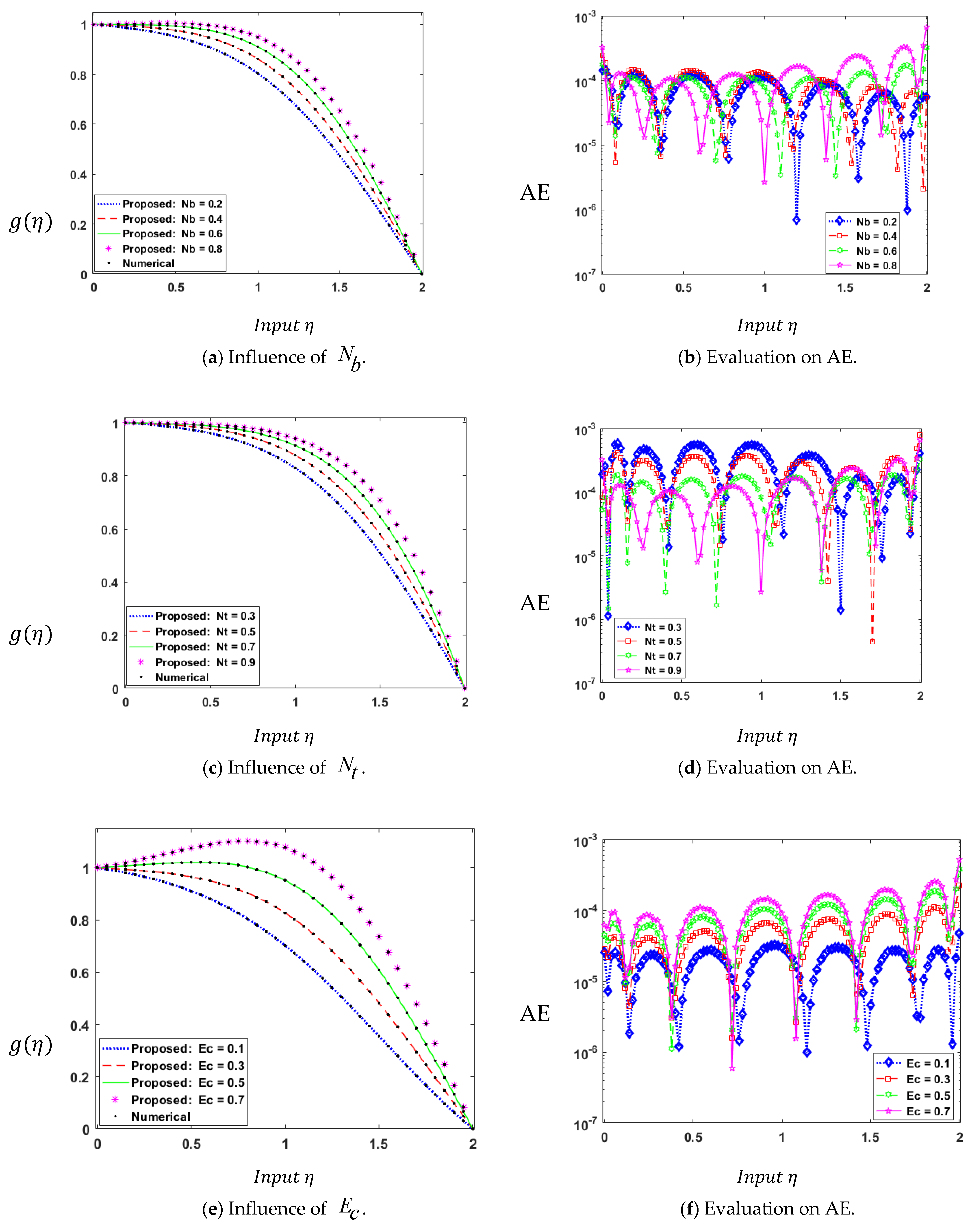
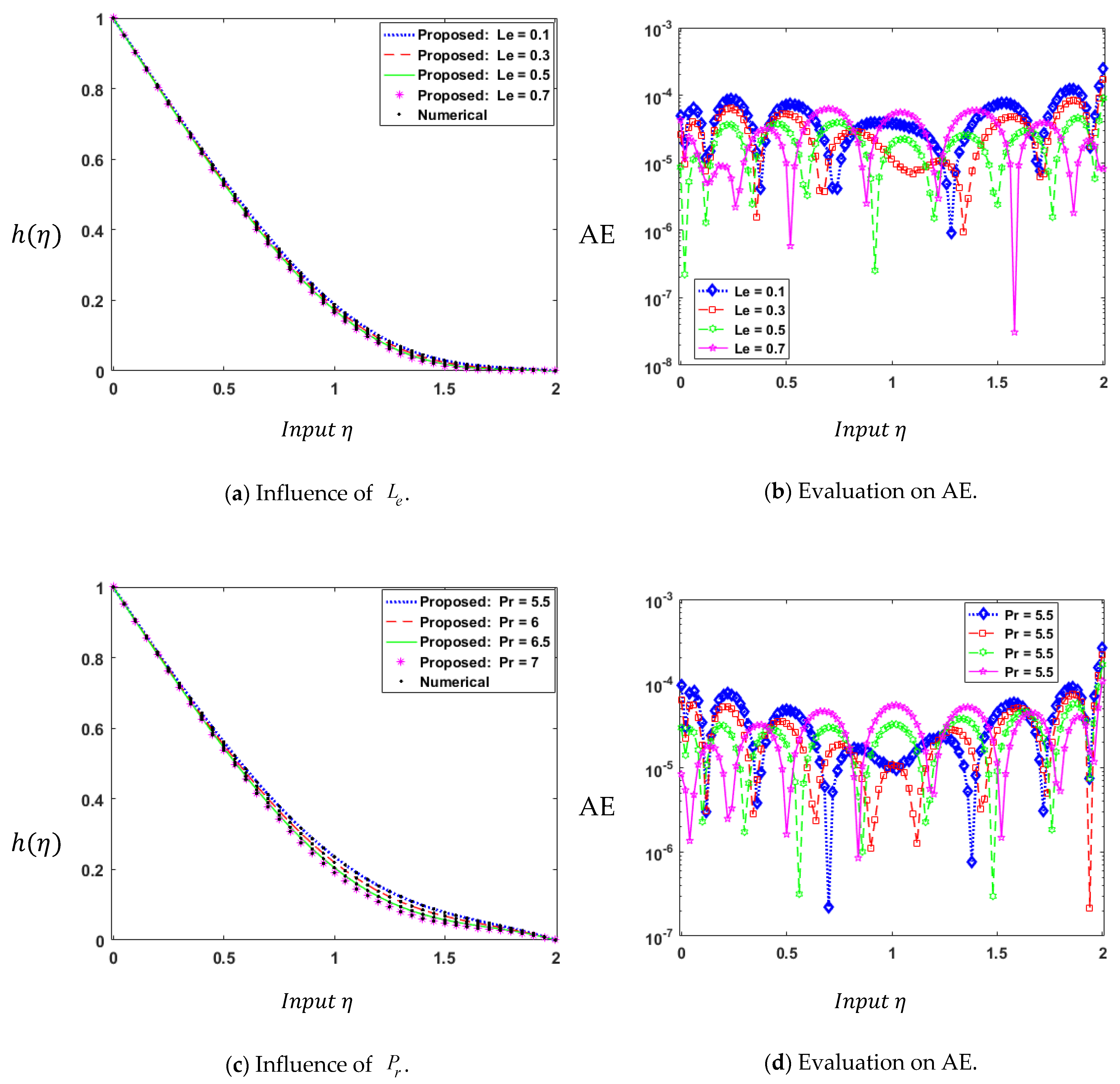
• Based on Hartmann number, Grashof numbers, concentration Grashoff factor, Lewis number, Brownian motion factor, Thermophoresis factor, Eckert number, Prandtl number, and other characteristics, the Adam’s solver is exploited to build a dataset for the designed TLMB-NN as an alternative to the dynamic of HTM-BFN;
• Modeling HTM-BFN for various scenarios by employing the TLMB-NN testing, validation, and training samples based procedures, and evaluation with orientation results rationalizes its perfection; and
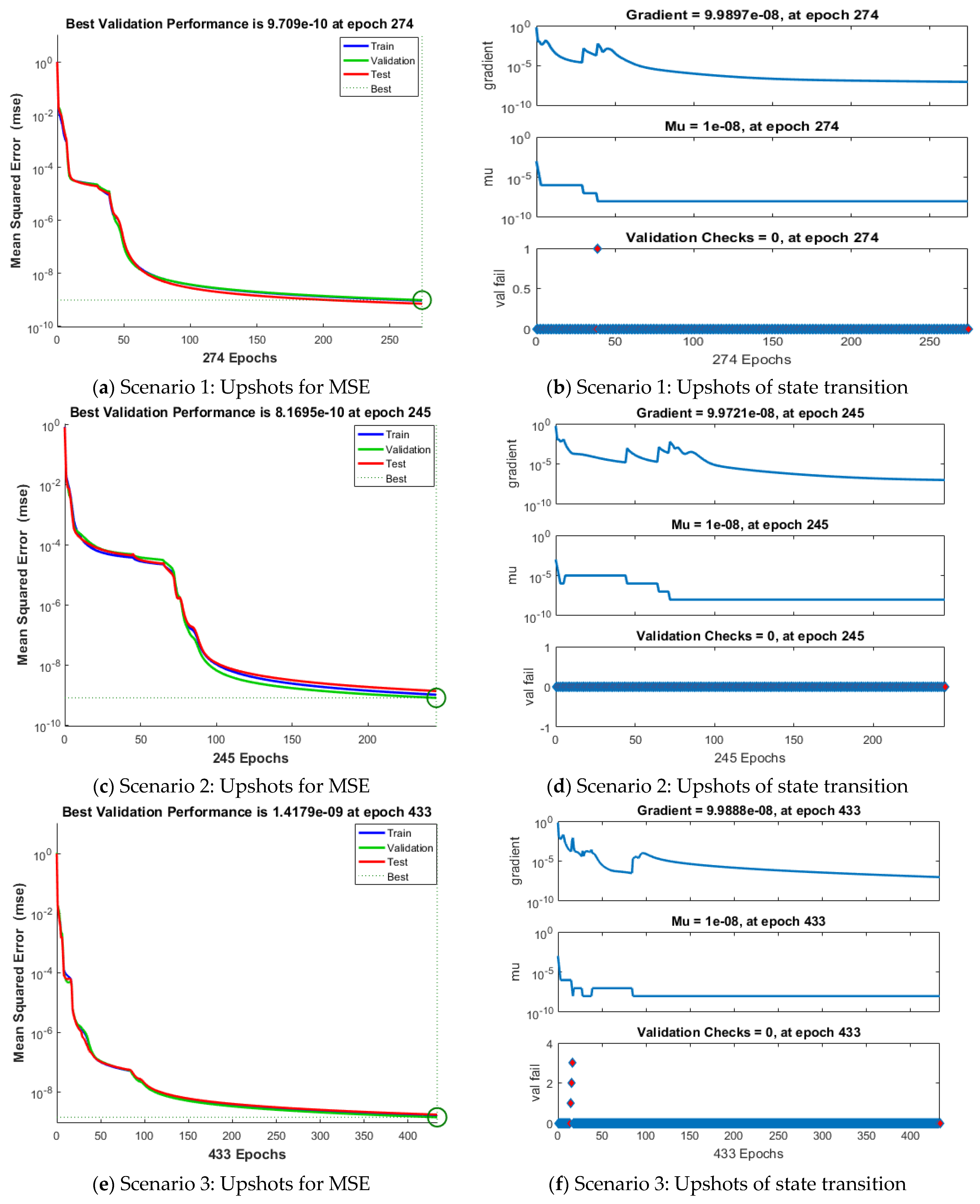
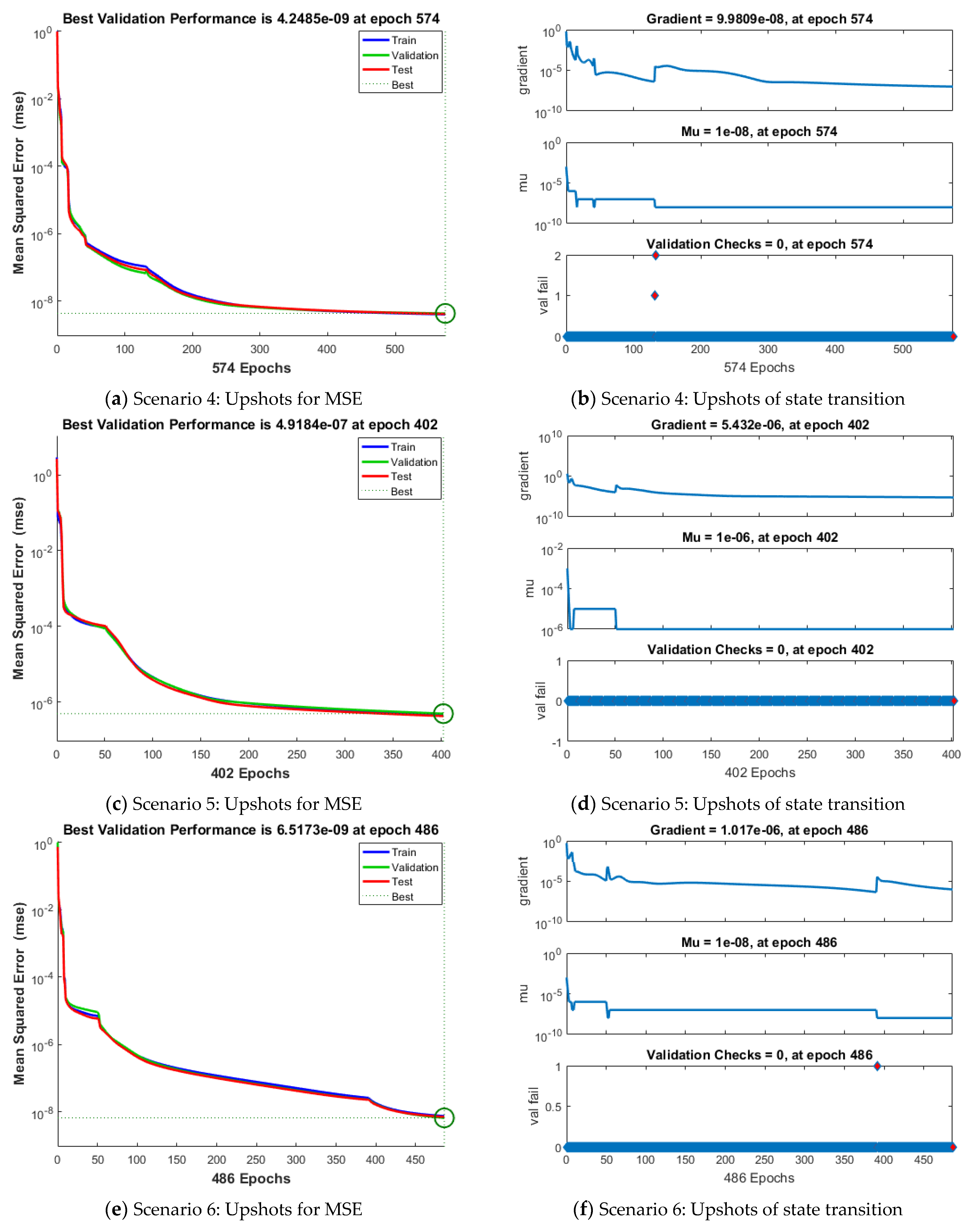
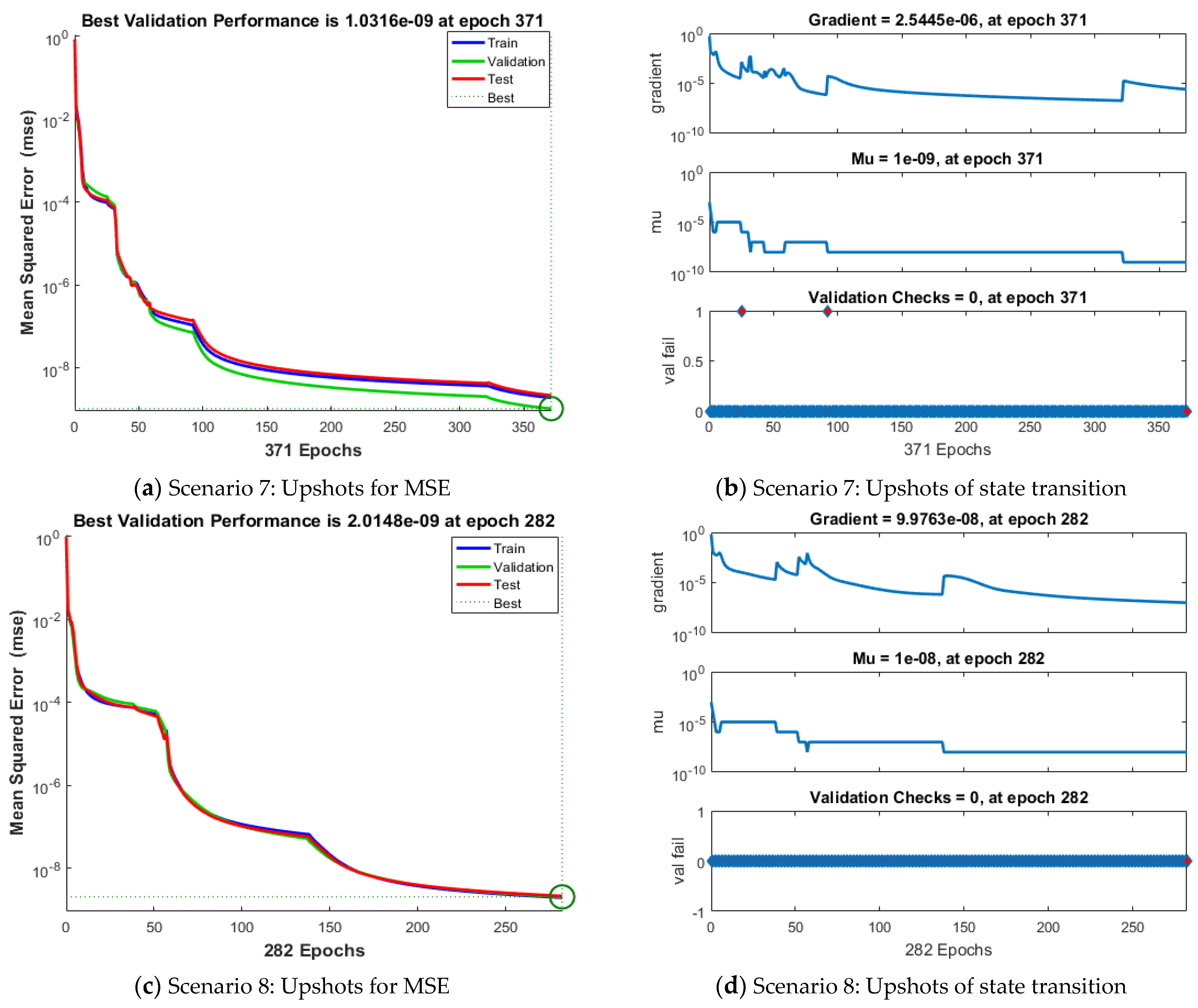
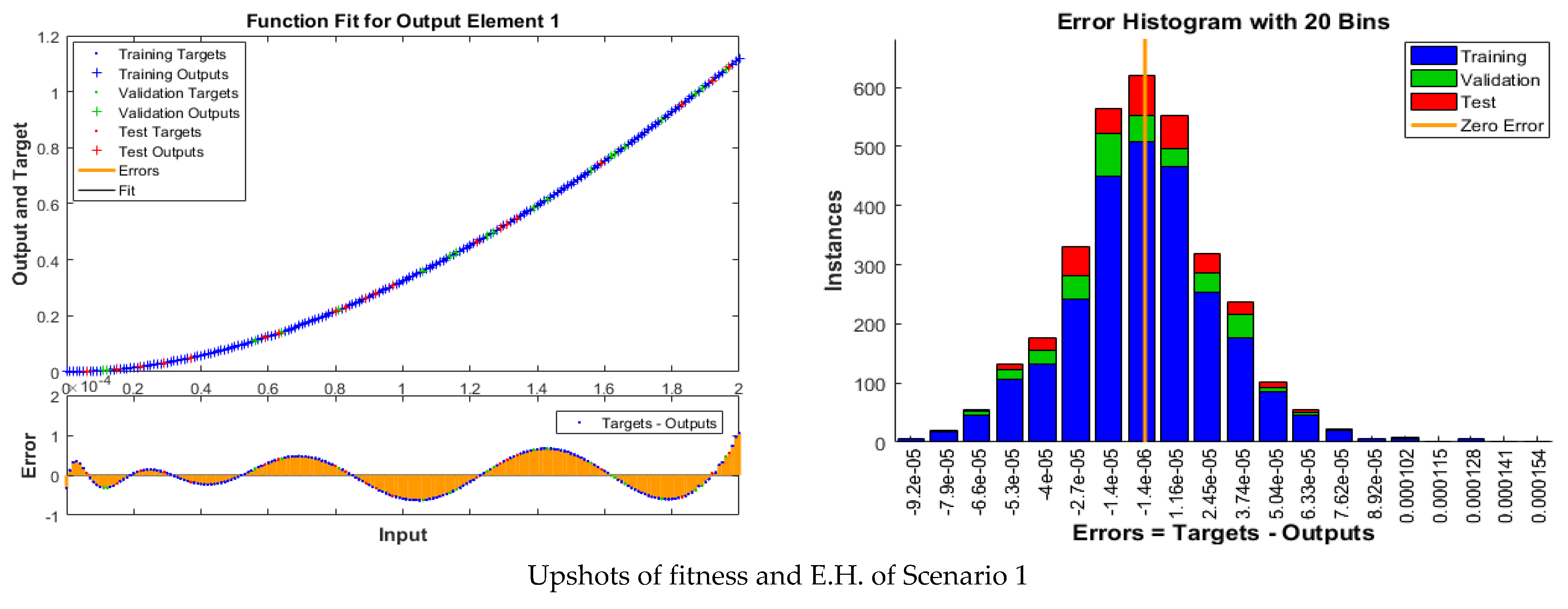
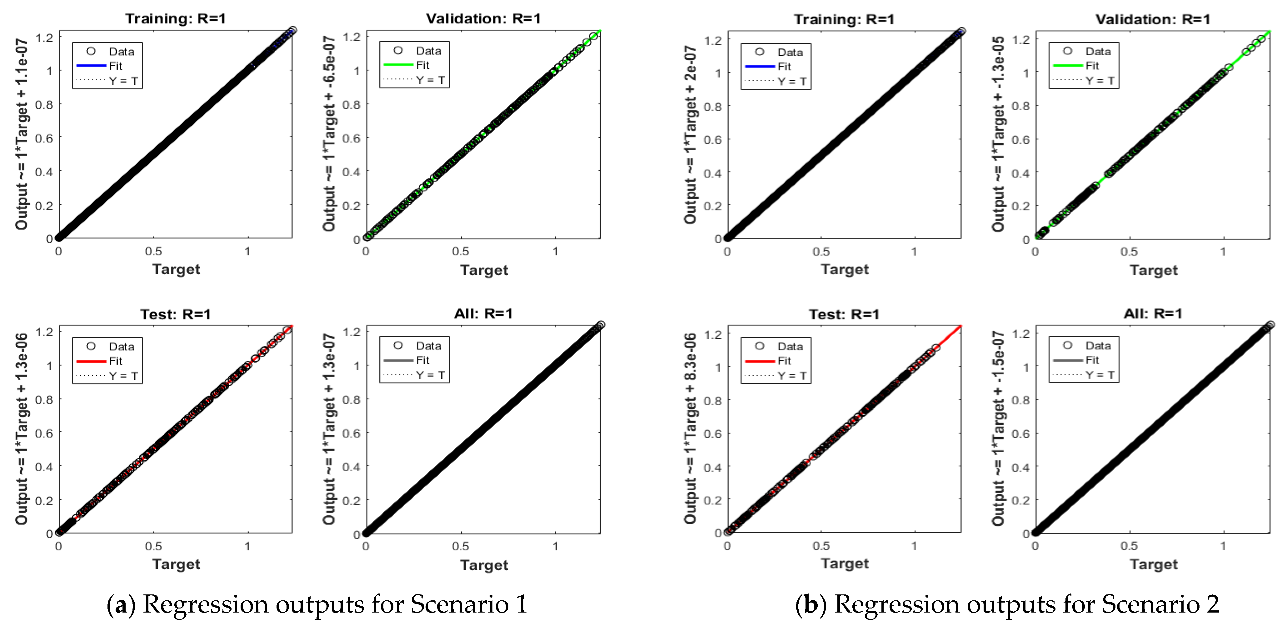
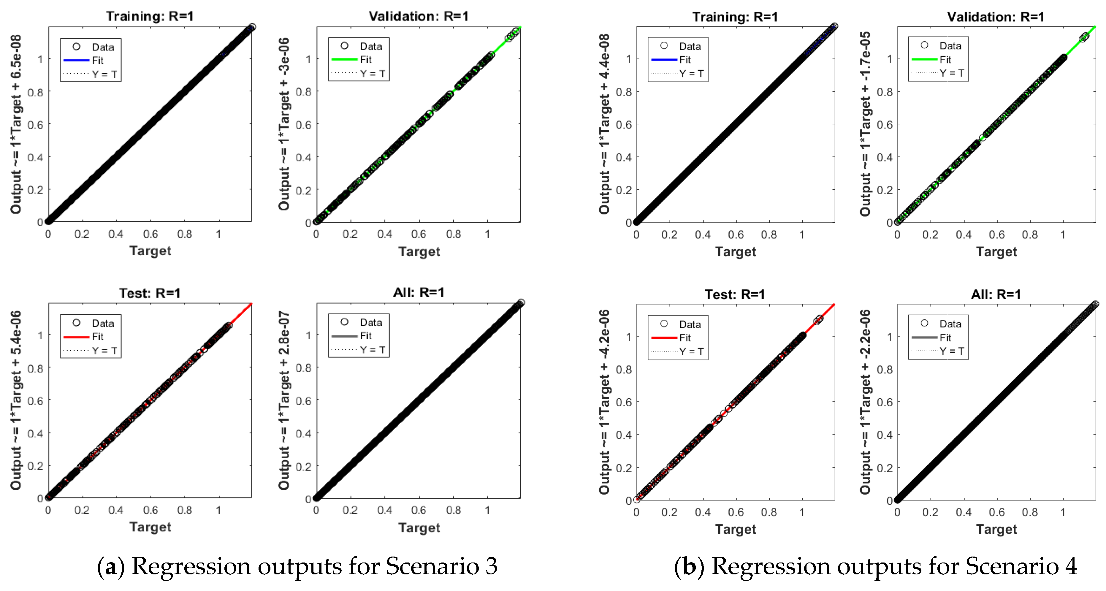
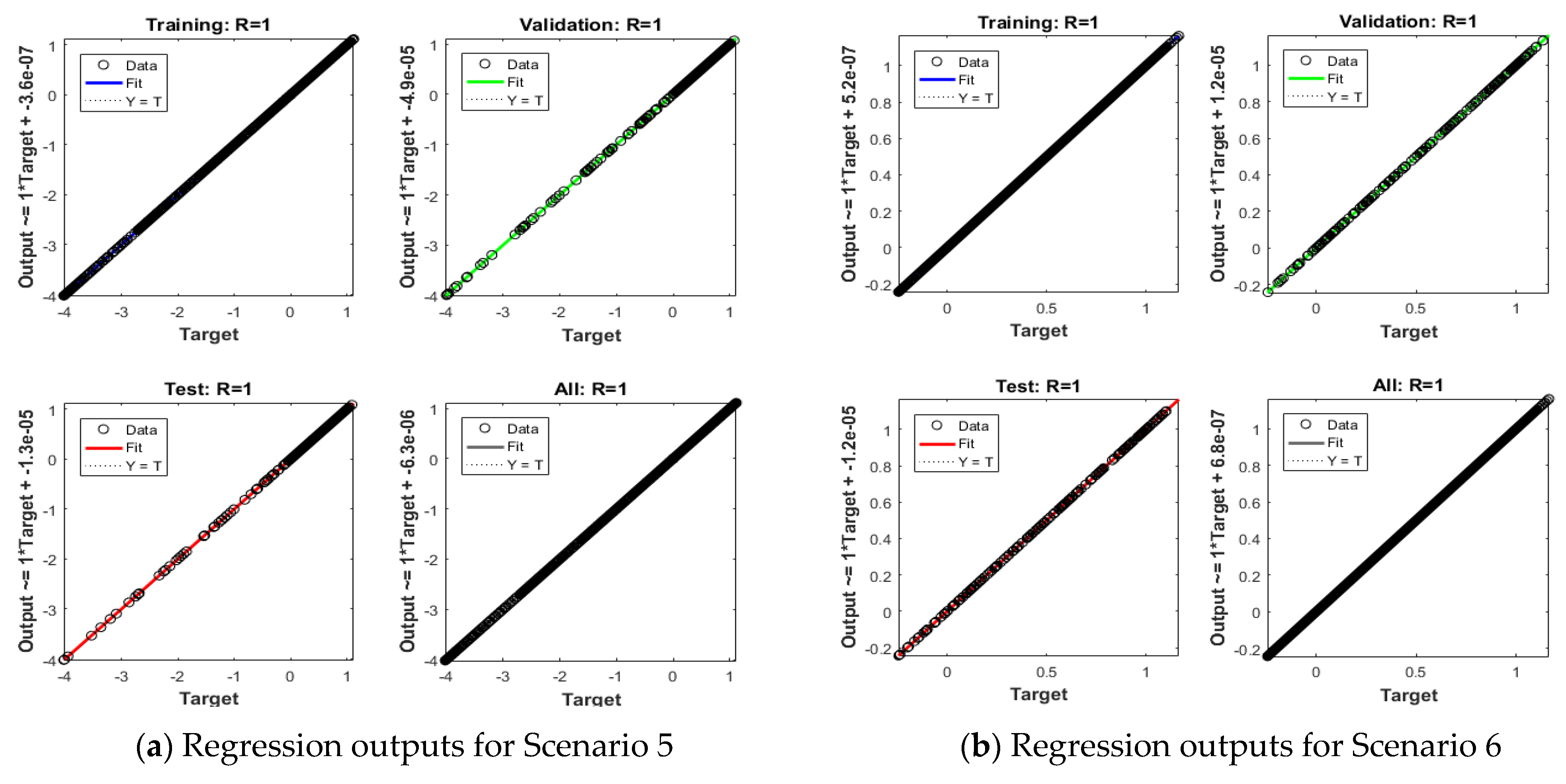
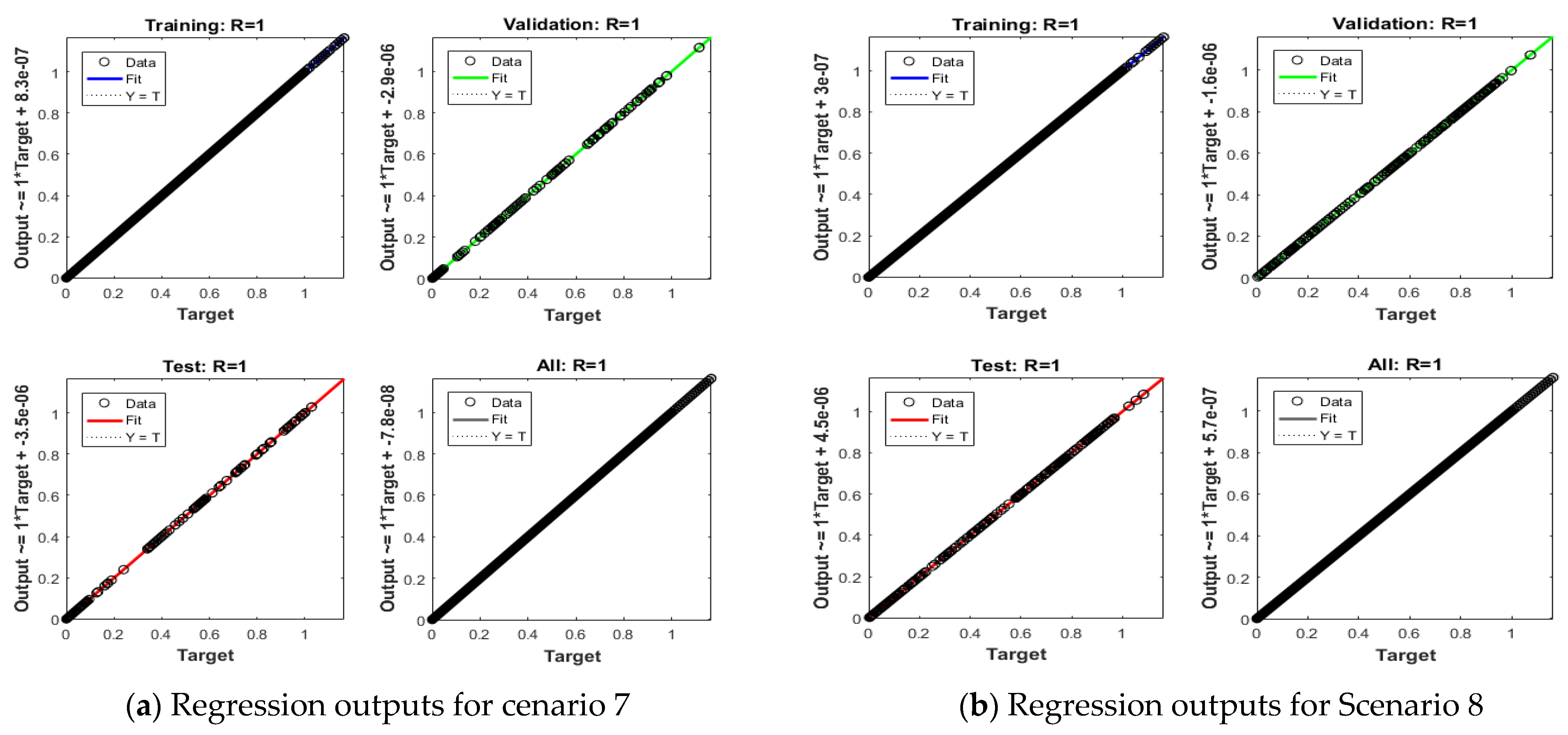
• The applicability of the suggested TLMB-NN to successfully represent the HTM-BFN model has supported by convergence graphs of calculated MSE, fitness, histograms, and regression metrics.

The subsequent research has been classified as follows: the interpretation and consequences of the HTM-BFN model problem are described in Section 2; Section 3 presents the solution approach as well as the impacts of the recommended TLMB-NN on numerous HTM-BFN alternatives; and Section 4 concludes with concluding observations and probable future study.

2. Mathematical Interpretation and Flow Assessment

Owing to a vertically moving flat permeable surface, we investigated the laminar, two-dimensional boundary coating flow of magneto hydrodynamics Maxwell nanofluid. The x-axis is parallel to the vertically moving flat plate, while the y-axis is orthogonal to it. Concentration and thermal buoyancy are other key factors. As consequences with thermal radiation and viscous dissipation, the fluid has been assumed to be heat absorbing. The fluid has given an unrestricted stream velocity ${\overline{U}}_e(\overline{x}),$ and the velocity ${\overline{U}}_w(\overline{x}),$ to the normally moving surface is given. The pattern of flow is presented via Figure 1. The dimensional boundary layer equations are given as [54].

$$\frac{\partial \overline{u}}{\partial \overline{x}}+\frac{\partial \overline{v}}{\partial \overline{y}}=0,\hspace{0.17em}$$

(1)

$$\begin{array}{l}\overline{u}\frac{\partial \overline{u}}{\partial \overline{x}}+\overline{v}\frac{\partial \overline{u}}{\partial \overline{y}}+\lambda ({\overline{u}}^2\frac{{\partial }^2\overline{u}}{\partial {\overline{x}}^2}+{\overline{v}}^2\frac{{\partial }^2\overline{u}}{\partial {\overline{y}}^2}+2\overline{uv}\frac{{\partial }^2\overline{u}}{\partial \overline{x}\partial \overline{y}}=-\frac{1}{\rho }\frac{\partial p}{\partial \overline{x}}\\ +\upsilon \left(\frac{{\partial }^2\overline{u}}{\partial {\overline{y}}^2}\right)-\frac{\overline{u}{B}_0^2\sigma }{\rho }+g_0{\beta }_T\left(\overline{T}-{\overline{T}}_{\infty }\right)+g_0{\beta }_c\left(\overline{C}-{\overline{C}}_{\infty }\right),\end{array}$$

(2)

$$\begin{array}{l}\left(\overline{u}\frac{\partial \overline{T}}{\partial \overline{x}}+\overline{v}\frac{\partial \overline{T}}{\partial \overline{y}}\right)=\alpha {\left(\frac{\partial \overline{T}}{\partial \overline{y}}\right)}^2+\frac{{\mu }_B}{{(\rho C_P)}_f}{\left(\frac{\partial \overline{u}}{\partial \overline{y}}\right)}^2+\frac{16a^{*}}{3k^{*}}\frac{\overline{T_{\infty }^3}}{{(\rho C_P)}_f}\\ \times \frac{{\partial }^2\overline{T}}{\partial {\overline{y}}^2}+\tau \left(D_B\frac{\partial \overline{T}}{\partial \overline{y}}\frac{\partial \overline{C}}{\partial \overline{y}}+{\left(\frac{\partial \overline{T}}{\partial \overline{y}}\right)}^2\right)\hspace{0.17em}-\frac{Q_0}{{(\rho C_P)}_f}(\overline{T}-{\overline{T}}_{\infty }),\end{array}$$

(3)

$$\overline{u}\frac{\partial \overline{C}}{\partial \overline{x}}+\hspace{0.17em}\overline{v}\frac{\partial \overline{C}}{\partial \overline{y}}=\hspace{0.17em}\left(\frac{{\partial }^2\overline{T}}{\partial {\overline{y}}^2}\right)\frac{D_T}{{\overline{T}}_{\infty }}+\frac{{\partial }^2\overline{C}}{\partial {\overline{y}}^2}{D}_B.$$

(4)

In terms of boundary conditions,

$$\begin{array}{l}\overline{u}=\hspace{0.17em}\hspace{0.17em}{\overline{U}}_w(\overline{x}),\hspace{0.17em}\hspace{0.17em}\hspace{0.17em}\hspace{0.17em}\hspace{0.17em}\overline{v}=\hspace{0.17em}\hspace{0.17em}{\overline{V}}_w(\overline{x}),\hspace{0.17em}\hspace{0.17em}\hspace{0.17em}\hspace{0.17em}\hspace{0.17em}\overline{T}\hspace{0.17em}=\hspace{0.17em}{\overline{T}}_w,\hspace{0.17em}\hspace{0.17em}\hspace{0.17em}\hspace{0.17em}\hspace{0.17em}\overline{C}\hspace{0.17em}=\hspace{0.17em}{\overline{C}}_w,\hspace{0.17em}\hspace{0.17em}\hspace{0.17em}\hspace{0.17em}\hspace{0.17em}\hspace{0.17em}at\hspace{0.17em}\hspace{0.17em}\overline{y}\hspace{0.17em}=\hspace{0.17em}0\\ \overline{u}\hspace{0.17em}\to \hspace{0.17em}{\overline{U}}_e(\overline{x}),\hspace{0.17em}\hspace{0.17em}\hspace{0.17em}\hspace{0.17em}\overline{T}\to \hspace{0.17em}{\overline{T}}_{\infty ,}\hspace{0.17em}\hspace{0.17em}\hspace{0.17em}\overline{C}\to \hspace{0.17em}{\overline{C}}_{\infty },\hspace{0.17em}\hspace{0.17em}\hspace{0.17em}\hspace{0.17em}\hspace{0.17em}\hspace{0.17em}\hspace{0.17em}\hspace{0.17em}\hspace{0.17em}\hspace{0.17em}\hspace{0.17em}\hspace{0.17em}\hspace{0.17em}\hspace{0.17em}\hspace{0.17em}\hspace{0.17em}\hspace{0.17em}\hspace{0.17em}\hspace{0.17em}\hspace{0.17em}\hspace{0.17em}\hspace{0.17em}\hspace{0.17em}\hspace{0.17em}\hspace{0.17em}at\hspace{0.17em}\hspace{0.17em}\overline{y}\to \hspace{0.17em}\infty ,\end{array}$$

(5)

where the wall dimensional velocity is ${\overline{U}}_w(\overline{x})$, and ${\overline{V}}_w(\overline{x})$ is dimensional mass flux velocity where for injection ${\overline{V}}_w(\overline{x})>0,$ and for suction ${\overline{V}}_w(\overline{x})<0$. The wall dimensional temperature and concentration are ${\overline{T}}_w,{\overline{C}}_w$. The temperature, concentration and dimensional free stream velocity are ${\overline{T}}_{\infty },{\overline{C}}_{\infty },{\overline{U}}_e\overline{(x)}$ respectively.

Equation (2) gives outside the boundary layer:

$$-\frac{1}{\rho }\frac{d\overline{p}}{d\overline{x}}=\lambda {\overline{U}}_e^2\frac{d^2{\overline{U}}_e}{d{\overline{x}}^2}+\overline{U}\frac{d{\overline{U}}_e}{d\overline{x}}+\frac{\sigma B_0^2}{\rho }{\overline{U}}_e,$$

(6)

Following are the variables in the boundary layer with no dimensions are:

$$\begin{array}{l}x=\frac{\overline{x}}{L},\hspace{0.17em}\hspace{0.17em}\hspace{0.17em}y=R_e^{\raisebox{1ex}{$1$}\!\left/ \!\raisebox{-1ex}{$2$}\right.}\left(\frac{\overline{y}}{L}\right),\hspace{0.17em}\hspace{0.17em}\hspace{0.17em}u=\frac{\overline{u}}{U_0},\hspace{0.17em}\hspace{0.17em}\hspace{0.17em}v=R_e^{\raisebox{1ex}{$1$}\!\left/ \!\raisebox{-1ex}{$2$}\right.}\left(\frac{\overline{v}}{U_0}\right),\\ u_e(x)=\frac{{\overline{U}}_e(\overline{x})}{U_0},\hspace{0.17em}\hspace{0.17em}\hspace{0.17em}{u}_w(x)=\frac{{\overline{U}}_w(\overline{x})}{U_0},\hspace{0.17em}\hspace{0.17em}\hspace{0.17em}{v}_w(x)=R_e^{\raisebox{1ex}{$1$}\!\left/ \!\raisebox{-1ex}{$2$}\right.}\frac{{\overline{V}}_w(\overline{x)}}{U_0},\hspace{0.17em}\\ \hspace{0.17em}\hspace{0.17em}\theta =\frac{\overline{T}-{\overline{T}}_{\infty }}{\overline{T_w}-{\overline{T}}_{\infty }},\hspace{0.17em}\hspace{0.17em}\hspace{0.17em}\varphi =\frac{\overline{C}-{\overline{C}}_{\infty }}{\overline{C_w}-{\overline{C}}_{\infty }},\hspace{0.17em}\hspace{0.17em}\hspace{0.17em}p=\frac{\overline{p}-p_{\infty }}{{\rho }_f{U}_0^2},\end{array}$$

(7)

where the characteristic velocity is $U_0$. We get the following system of equations by merging Equations (6) and (7):

$$\frac{\partial u}{\partial x}+\frac{\partial v}{\partial y}=0,\hspace{0.17em}$$

(8)

$$\begin{array}{l}u\frac{\partial u}{\partial x}+v\frac{\partial u}{\partial y}+\frac{\lambda U_0}{L}\left(u^2\frac{{\partial }^{2}u}{\partial x^2}+v^2\frac{{\partial }^{2}u}{\partial y^2}+2uv\frac{{\partial }^{2}u}{\partial y\partial x}\right)\\ -\left(\frac{\lambda U_0}{L}\right)u_e^2\frac{d^2{u}_e}{d{x}^2}-u_e\frac{d{u}_e}{dx}=+\frac{{\partial }^{2}u}{\partial y^2}+\left(\frac{\sigma B_0^{2}L}{\rho U_0}\right)(u_e-u)\\ +({\overline{T}}_w-{\overline{T}}_{\infty })\frac{g_0{\beta }_{T}L}{U_0^2}\theta +({\overline{C}}_w-{\overline{C}}_{\infty })\frac{g_0{\beta }_{c}L}{U_0^2}\varphi ,\hspace{0.17em}\end{array}$$

(9)

$$\begin{array}{l}u\frac{\partial \theta }{\partial x}+v\frac{\partial \theta }{\partial y}=\frac{1}{P_r}\frac{{\partial }^2\theta }{\partial y^2}+\frac{U_0^2}{C_p({\overline{T}}_w-{\overline{T}}_{\infty })}{\left(\frac{\partial u}{\partial y}\right)}^2\\ +\frac{4R}{3P_r}\frac{{\partial }^2\theta }{\partial y^2}+\frac{\partial \varphi }{\partial y}\frac{\partial \theta }{\partial y}{N}_b+N_t{\left(\frac{\partial \theta }{\partial y}\right)}^2-\frac{Q_{0}L}{{(\rho C_p)}_f}\theta ,\hspace{0.17em}\end{array}$$

(10)

$$u\frac{\partial \varphi }{\partial x}+v\frac{\partial \varphi }{\partial y}\hspace{0.17em}=\hspace{0.17em}\frac{1}{P_r}\left(\frac{1}{L_e}\frac{{\partial }^2\varphi }{\partial y^2}+\frac{N_T}{N_b{L}_e}\frac{{\partial }^2\theta }{\partial y^2}\right).$$

(11)

The dimensionless boundary conditions have obtained by applying Equation (7) in Equation (5):

$$\begin{array}{l}u=\hspace{0.17em}\hspace{0.17em}{u}_w(x),\hspace{0.17em}\hspace{0.17em}\hspace{0.17em}\hspace{0.17em}\hspace{0.17em}\hspace{0.17em}\hspace{0.17em}v\hspace{0.17em}=\hspace{0.17em}{v}_w(x),\hspace{0.17em}\hspace{0.17em}\hspace{0.17em}\hspace{0.17em}\hspace{0.17em}\hspace{0.17em}\theta \hspace{0.17em}=\hspace{0.17em}1,\hspace{0.17em}\hspace{0.17em}\hspace{0.17em}\hspace{0.17em}\hspace{0.17em}\varphi \hspace{0.17em}=\hspace{0.17em}1,\hspace{0.17em}\hspace{0.17em}\hspace{0.17em}\hspace{0.17em}\hspace{0.17em}at\hspace{0.17em}\hspace{0.17em}y\hspace{0.17em}=\hspace{0.17em}0\\ u\hspace{0.17em}\to \hspace{0.17em}{u}_e(x),\hspace{0.17em}\hspace{0.17em}\hspace{0.17em}\hspace{0.17em}\hspace{0.17em}\hspace{0.17em}\hspace{0.17em}\theta \hspace{0.17em}\to \hspace{0.17em}0,\hspace{0.17em}\hspace{0.17em}\hspace{0.17em}\hspace{0.17em}\hspace{0.17em}\hspace{0.17em}\hspace{0.17em}\hspace{0.17em}\hspace{0.17em}\hspace{0.17em}\hspace{0.17em}\hspace{0.17em}\varphi \to \hspace{0.17em}0,\hspace{0.17em}\hspace{0.17em}\hspace{0.17em}\hspace{0.17em}\hspace{0.17em}\hspace{0.17em}\hspace{0.17em}\hspace{0.17em}\hspace{0.17em}\hspace{0.17em}\hspace{0.17em}\hspace{0.17em}\hspace{0.17em}\hspace{0.17em}\hspace{0.17em}\hspace{0.17em}\hspace{0.17em}as\hspace{0.17em}\hspace{0.17em}y\to \hspace{0.17em}\infty \hspace{0.17em}.\end{array}$$

(12)

We suppose that $u_w(x),$ and $u_e(x),$ have the subsequent structure $u_w(x)=U_w{x}^{\raisebox{1ex}{$1$}\!\left/ \!\raisebox{-1ex}{$3$}\right.},$ and $u_e(x)=U_e{x}^{\raisebox{1ex}{$1$}\!\left/ \!\raisebox{-1ex}{$3$}\right.},$ where the dimensionless constants are $U_w,$ $U_e$. The similarity transformations are introduced here as:

$$\begin{array}{l}\psi =U_e^{\frac{1}{2}}{x}^{\frac{2}{3}}f(\eta ),\hspace{0.17em}\hspace{0.17em}\hspace{0.17em}\eta =U_e^{\frac{1}{2}}{x}^{-\frac{1}{3}}y,\hspace{0.17em}\hspace{0.17em}\hspace{0.17em}\theta =g(\eta ),\hspace{0.17em}\hspace{0.17em}\\ \hspace{0.17em}\varphi =h(\eta ),\hspace{0.17em}\hspace{0.17em}u=\frac{\partial \psi }{\partial y},\hspace{0.17em}\hspace{0.17em}\hspace{0.17em}v=-\frac{\partial \psi }{\partial y},\end{array}$$

(13)

Thus, we get $v_w(x)=-\frac{2}{3}{U}_e^{\frac{1}{2}}{x}^{-\raisebox{1ex}{$1$}\!\left/ \!\raisebox{-1ex}{$3$}\right.}s,$ where dimensionless transpiration parameter is $s,$ and the suction and injection cases are given by $s>0,\hspace{0.17em}s<0$, correspondingly. Equations (8)–(12) yield the form, after manipulating the similarity transformations given in Equation (13),

$$\begin{array}{l}3\left({f^{\prime }}^2-1\right)-6f{f}^{″}+2\beta \left(\eta {f^{\prime }}^2{f}^{″}+1-{f^{\prime }}^3+2f^{‴}{f}^2\right)\\ -9\left(\left(M(1-f^{\prime }\right)f^{‴}+G_{T}g+G_{c}h\right)=0,\end{array}$$

(14)

$$\frac{1}{P_r}\left(1+\frac{4R}{3}\right)g^{″}+E_c{f}^{″2}+h^{\prime }{g}^{\prime }{N}_b+g^{\prime 2}{N}_t+\frac{2}{3}f{g}^{\prime }-Hg=0,$$

(15)

$$h^{″}+g^{″}\frac{N_t}{N_b}+\frac{2}{3}{L}_e{P}_{r}f{h}^{\prime }=0.$$

(16)

Their relative boundary conditions are given as:

$$\begin{array}{l}f(\eta )=s,\hspace{0.17em}\hspace{0.17em}\hspace{0.17em}\hspace{0.17em}h(\eta )=1,\hspace{0.17em}\hspace{0.17em}\hspace{0.17em}g(\eta )=1,\hspace{0.17em}\hspace{0.17em}\hspace{0.17em}{f}^{\prime }(\eta )=\gamma ,\hspace{0.17em}\hspace{0.17em}\hspace{0.17em}at\hspace{0.17em}\eta =0\\ f^{\prime }(\eta )=1,\hspace{0.17em}\hspace{0.17em}g(\eta )=h(\eta )=0,\hspace{0.17em}\hspace{0.17em}\hspace{0.17em}\hspace{0.17em}as\hspace{0.17em}\hspace{0.17em}\eta \to \infty ,\hspace{0.17em}\hspace{0.17em}\end{array}\}$$

(17)

where for moving flat plate $\gamma =\frac{U_w}{U_e},$ is non-dimensional factor. If free stream and moving flat surface are parallel, then $\gamma >0,$ but, if not parallel, then $\gamma <0,$ and for plate at rest $\gamma =0$. The dimensionless parameters are specified as under:

$$\begin{array}{l}M=\frac{L{B}_0^2\sigma }{U_0{U}_e{x}^{-\frac{2}{3}}\rho },\hspace{0.17em}\hspace{0.17em}\hspace{0.17em}\hspace{0.17em}\hspace{0.17em}\hspace{0.17em}\beta =\frac{\lambda U_0{U}_e{x}^{-\frac{2}{3}}}{L},\hspace{0.17em}\hspace{0.17em}\hspace{0.17em}\hspace{0.17em}\hspace{0.17em}\hspace{0.17em}{G}_c=\frac{{\beta }_{c}L{g}_0({\overline{C}}_w-{\overline{C}}_{\infty })}{U_0^2{U}_e^2{x}^{-\frac{2}{3}}},\hspace{0.17em}\\ G_T=\frac{{\beta }_{T}L{g}_0({\overline{T}}_w-{\overline{T}}_{\infty })}{U_0^2{U}_e^2{x}^{-\frac{2}{3}}},\hspace{0.17em}\hspace{0.17em}\hspace{0.17em}\hspace{0.17em}{L}_e=\frac{\alpha }{D_B},\hspace{0.17em}\hspace{0.17em}\hspace{0.17em}{P}_r=\frac{\upsilon }{\alpha },\hspace{0.17em}\hspace{0.17em}\hspace{0.17em}\hspace{0.17em}\hspace{0.17em}\hspace{0.17em}\hspace{0.17em}{N}_t=\frac{\tau ({\overline{T}}_w-{\overline{T}}_{\infty })D_T}{\upsilon {\overline{T}}_{\infty }}\hspace{0.17em},\\ N_b=\frac{\tau ({\overline{C}}_w-{\overline{C}}_{\infty })D_B}{\upsilon },\hspace{0.17em}\hspace{0.17em}\hspace{0.17em}{E}_c=\frac{U_0^2{U}_e^2}{C_p-\raisebox{1ex}{$2$}\!\left/ \!\raisebox{-1ex}{$3$}\right.({\overline{T}}_w-{\overline{T}}_{\infty })},\hspace{0.17em}\hspace{0.17em}\hspace{0.17em}\hspace{0.17em}\\ H=\frac{Q_{0}L}{U_0{U}_e{x}^{-\frac{2}{3}}{(\rho C_p)}_f},\hspace{0.17em}\hspace{0.17em}\hspace{0.17em}R=\frac{4{\sigma }^{*}{\overline{T}}_{\infty }^3}{kf{k}^{*}}\end{array}$$

(18)

where M is the Hartmann number, β denote the Deborah number, G_c and G_T represent the concentration and thermal Grashoff parameters, Le denote the Lewis number, P_r show the Prandtl number, N_t and N_b represent the Thermophoresis and Brownian motion parameters, Eckert number is indicated by E_c, H display the heat-absorption factor, and R signify the Radiation parameter. The Nusselt number $N_{ux},$ is specify as:

$$N_{ux}=\frac{x{q}_w}{k(T_w-T_{\infty })},$$

where

$$q_w=-k\left(1+\frac{16{\sigma }^{*}{T}_{\infty }^3}{3k^{*}kf}\right){\left(\frac{\partial T}{\partial y}\right)}_{y=0},$$

And

$${\mathrm{Re}}_x^{-\frac{1}{2}}N{u}_x=-\left(1+\frac{4R}{3}\right)g^{\prime }(0).$$

the Sherwood quantity is expressed as:

$$S{h}_x=\frac{x{h}_m}{D_B(C_w-C_{\infty })},\hspace{0.17em}$$

where, $h_m=-D_B{\left(\frac{\partial C}{\partial y}\right)}_{y=0},\hspace{0.17em}\hspace{0.17em}$ and $\hspace{0.17em}{\mathrm{Re}}_x^{-\frac{1}{2}}S{h}_x=-h^{\prime }(0).$

In above $q_w,\hspace{0.17em}{h}_m$ are the mathematical representations, which describe the heat slope of wall and mass of wall incline, correspondingly.

3. Solution Methodology

In the shape of a neural network structure, Figure 2 displays the suggested TLMB-NN model. The suggested TLMB-NN is accomplished by operating ‘nf tool’, i.e., in Mat lab’s neural network (NN) toolbox, setting a procedure for fitting NN tools, whereas the Levenberg–Marquardt with backpropagation is concluded, finding out the weight of neural networks. In Figure 3a, the suggested TLMB-NN model and the mathematical model along with concern geometry have displayed and in Figure 3b the overall elaboration of flow demonstration has presented, while the necessary details of the size and structure of the networks is tabulated in

Table 1. Size and structural details of the networks.

Index	Description
Layer structure	One input, one output, and one hidden layer
Hidden neuron	10–20
Validation	10-fold cross validation
Input grid	201 points
Output grid	16 × 201 points
Training samples	80%
Validation samples	10%
Testing samples	10%
Leaning methodology	Levenberg–Marquardt
Label target data	Created with Adams numerical method

.

For fixed values of ${\beta }_{D }$ = 0.5, $R$= 0.6, and H = 0.3 are exercised for the variation of distinct parameters $M$, $G_T$, $G_c$, $N_t$, $N_b$, $E_c$, $L_e$, and $P_r$ respectively, with four cases of HTM-BFN model, individually. With replacements for all alternatives, as stated in Table 1, the suggested TLMB-NN is operated to solve differential Equations (14)–(16) of the flow paradigm for eight scenarios, exploiting the Adams numerical solver method [55,56,57]; that is in Mathematica software the command ‘Nonlinear differential system (ND Solver)’ is exercised with time interval 0.01 to generate dataset of TLMB-NN for inputs between 0 and 2 as deliberate below in Table 1 and

Table 2. Scenarios interpretation beside with cases for HTM-BFN model with MHD.

Scenarios	Cases	Physical Quantities of Concern
		$\mathit{M}$	${\mathit{G}}_{\mathit{T}}$	${\mathit{G}}_{\mathit{c}}$	${\mathit{N}}_{\mathit{b}}$	${\mathit{N}}_{\mathit{t}}$	${\mathit{E}}_{\mathit{c}}$	${\mathit{L}}_{\mathit{e}}$	${\mathit{P}}_{\mathit{r}}$
1	C1	0.1	0.2	0.2	0.1	0.1	0.3	0.3	6.5
	C2	0.3	0.2	0.2	0.1	0.1	0.3	0.3	6.5
	C3	0.5	0.2	0.2	0.1	0.1	0.3	0.3	6.5
	C4	0.7	0.2	0.2	0.1	0.1	0.3	0.3	6.5
2	C1	0.3	0.1	0.2	0.1	0.1	0.3	0.3	6.5
	C2	0.3	0.2	0.2	0.1	0.1	0.3	0.3	6.5
	C3	0.3	0.3	0.2	0.1	0.1	0.3	0.3	6.5
	C4	0.3	0.4	0.2	0.1	0.1	0.3	0.3	6.5
3	C1	0.3	0.2	0.1	0.1	0.1	0.3	0.3	6.5
	C2	0.3	0.2	0.2	0.1	0.1	0.3	0.3	6.5
	C3	0.3	0.2	0.3	0.1	0.1	0.3	0.3	6.5
	C4	0.3	0.2	0.4	0.1	0.1	0.3	0.3	6.5
4	C1	0.3	0.2	0.2	0.2	0.1	0.3	0.3	6.5
	C2	0.3	0.2	0.2	0.4	0.1	0.3	0.3	6.5
	C3	0.3	0.2	0.2	0.6	0.1	0.3	0.3	6.5
	C4	0.3	0.2	0.2	0.8	0.1	0.3	0.3	6.5
5	C1	0.3	0.2	0.2	0.1	0.3	0.3	0.3	6.5
	C2	0.3	0.2	0.2	0.1	0.5	0.3	0.3	6.5
	C3	0.3	0.2	0.2	0.1	0.7	0.3	0.3	6.5
	C4	0.3	0.2	0.2	0.1	0.9	0.3	0.3	6.5
6	C1	0.3	0.2	0.2	0.1	0.1	0.1	0.3	6.5
	C2	0.3	0.2	0.2	0.1	0.1	0.3	0.3	6.5
	C3	0.3	0.2	0.2	0.1	0.1	0.5	0.3	6.5
	C4	0.3	0.2	0.2	0.1	0.1	0.7	0.3	6.5
7	C1	0.3	0.2	0.2	0.1	0.1	0.3	0.1	6.5
	C2	0.3	0.2	0.2	0.1	0.1	0.3	0.3	6.5
	C3	0.3	0.2	0.2	0.1	0.1	0.3	0.5	6.5
	C4	0.3	0.2	0.2	0.1	0.1	0.3	0.7	6.5
8	C1	0.3	0.2	0.2	0.1	0.1	0.3	0.3	5.5
	C2	0.3	0.2	0.2	0.1	0.1	0.3	0.3	6
	C3	0.3	0.2	0.2	0.1	0.1	0.3	0.3	6.5
	C4	0.3	0.2	0.2	0.1	0.1	0.3	0.3	7

. With a set of 10 hidden neurons, for training 80% data values, 10% individually for validation and testing the solutions for $f^{\prime }, g$ and $h$ for 201 input points are informally scattered.

4. Results and Discussion

The TLMB-NN outcomes for the HTM-BFN model have been shown in Figure 4, Figure 5, Figure 6, Figure 7, Figure 8 and Figure 9 for different circumstances (scenarios) (1 to 8). Figure 4, Figure 5 and Figure 6 show the outcomes of eight scenarios in terms of performance and transition phases: $M$, $G_T$, $G_c$, $N_t$, $N_b$, $E_c$, $L_e$, and $P_r$. The fitting plots and error histograms in Figure 7, Figure 8 and Figure 9 were stated in terms of solution with error for four distinct situations, however, the regression estimations exhibited for four unique HTM-BFN model with MHD, collections in Figure 10, Figure 11 and Figure 12. In addition, for every HTM-BFN model scenario,

Table 3. Outcomes of TLMB-NN for eight scenarios (HTM-BFN model) with MHD.

Scenarios	MSE Level			Execution	Gradient	Mu	Epoch	Time
	Training	Validation	Testing
$M$	9.249 × 10−10	9.709 × 10−10	7.092 × 10−10	9.25 × 10−10	9.99 × 10−8	1.00 × 10−8	274	12
$G_T$	1.039 × 10−9	8.169 × 10−10	1.380 × 10−9	1.04 × 10−9	9.97 × 10−8	1.00 × 10−8	245	12
$G_c$	1.677 × 10−9	1.417 × 10−9	1.742 × 10−9	1.68 × 10−9	9.99 × 10−8	1.00 × 10−8	433	32
$N_b$	3.9720 × 10−7	4.248 × 10−9	4.092 × 10−9	3.97 × 10−9	9.98 × 10−8	1.00 × 10−8	574	31
$N_t$	4.607 × 10−7	4.918 × 10−7	4.232 × 10−7	4.61 × 10−7	5.43 × 10−6	1.00 × 10−6	402	29
$E_c$	7.368 × 10−9	6.517 × 10−9	6.931 × 10−9	7.37 × 10−9	1.02 × 10−6	1.00 × 10−8	486	20
$L_e$	1.883 × 10−9	1.031 × 10−9	2.151 × 10−9	1.88 × 10−9	2.54 × 10−9	1.00 × 10−10	371	27
$P_r$	1.931 × 10−9	2.014 × 10−9	2.113 × 10−9	1.93 × 10−9	9.98 × 10−8	1.00 × 10−8	282	12

lists the convergence achieve parameter in terms of mean square error (MSE), execution, performed period, performance duration, back propagation, and temporal complexity gauges for scenarios 1 to 8.

In Figure 4a,c,e, Figure 5a,c,e and Figure 6a,c,e for test processes, the convergence of MSE, validation, and training progressions for eight scenarios of the HTM-BFN model with MHD are considered. MSE nearby 9.7 × 10⁻¹⁰, 8.16 × 10⁻¹⁰, 1.41 × 10⁻⁹, 4.24 × 10⁻⁹, 4.91 × 10⁻⁷, 6.51 × 10⁻⁹, 1.03 × 10⁻⁹, and 2 × 10⁻⁹, with epochs 274, 245, 433, 574, 402, 486, 371, and 282, correspondingly, provided the finest network performance. The lower the MSE number, the more precise and effective the performance of the given approach may be. The estimates of step size Mu and Levenberg–Marquardt gradient are compactly (10⁻⁸, 10⁻⁸, 10⁻⁸, 10⁻⁸, 10⁻⁶, 10⁻⁸, 10⁻⁹, and 10⁻⁸) and (9.98 × 10⁻⁸, 9.97 × 10⁻⁸, 9.98 × 10⁻⁸, 9.98 × 10⁻⁸, 5.43 × 10⁻⁶, 1.01 × 10⁻⁶, 2.54 × 10⁻⁶, and 9.97 × 10⁻⁸) are presented in Figure 4b,d,f, Figure 5b,d,f and Figure 6b,d,f. The aforesaid outputs and graphical validations identify the authenticity that TLMB-NN is efficient, precise, and convergent for each case of HTM-BFN paradigm.

Figure 7, Figure 8 and Figure 9 demonstrate the effectiveness of the HTM-BFN model by comparing the generated outcomes of eight different scenarios for inputs ranging from 0 to 2 with a step range of 0.01 to reference numerical Adams method outcomes and related outcomes, as well as the error dynamics plot. The highest error for test, train, and validation gauges achieved through suggested TLMB-NN for eight scenarios of the design paradigm is less than 9 × 10⁻¹⁰, 8 × 10⁻¹⁰, 1 × 10⁻⁹, 4 × 10⁻⁹, 4 × 10⁻⁷, 7 × 10⁻⁹, 2 × 10⁻⁹, and 2 × 10⁻⁹, while the error dynamics and outcomes of HTM-BFN model for eight detached scenarios is also inspected for every input point aside from error histograms are shown in Figure 7, Figure 8 and Figure 9, correspondingly. The average value of error bin about comparison zero line has error nearby for eight distinct situations of the HTM-BFN model −1.4 × 10⁻⁶, 3.06 × 10⁻⁶, 5.98 × 10⁻⁶, −6.3 × 10⁻⁶, 2.6 × 10⁻⁴, −1.6 × 10⁻⁵, −1.2 × 10⁻⁶, and 4.07 × 10⁻⁶. Correlation analyses have frequently used to summarize the analysis inside regression analyses. Figure 10 through Figure 13 show the impacts of the HTM-BFN model’s eight related alternatives. The correlation R-values are continuously near to unity, implying that the optimal value for training, testing, and validation for precise modeling is close to unity, which explains how effectively TLMB-NN resolves the HTM-BFN model.

Furthermore, the associated numerical data in Table 3 demonstrate that MSE performance for the suggested TLMB-NN technique is approximately 10–10 for various HTM-BFN model situations (1 to 8). The numerical results in Table 3 demonstrate that, while solving the HTM-BFN model, TLMB-NN executions are sound.

The effects of TLMB-NN are shown in Figure 14, Figure 15 and Figure 16, respectively, for velocity distribution $f^{\prime }\left(\eta \right),$ temperature distribution $g\left(\eta \right),$ and concentration distribution $h\left(\eta \right)$ for all eight scenarios of the (HTM-BFN) paradigm. In Figure 14a,c,e, the influence of velocity profile $f^{\prime }\left(\eta \right)$ on the variation of Hartmann number $M$, thermal Grashoff parameter $G_T$ and concentration Grashoff parameter $G_c$ for scenarios 1, 2, and 3 of the (HTM-BFN) model is measured; on the other hand, in Figure 14b,d,f, the related values of AE are plotted in order to attain the performance of the HTM-BFN model approach.

Figure 14a,c,e illustrates graphs of velocity versus various physical parameter values. As seen in Figure 14a–c, the velocity increases in magnitude by increasing the values of $M$, $G_T$ and $G_c$. Figure 14a depicts the alteration in Hartmann number for velocity distribution. When the magnetic field’s effect is increased, the flow accelerates, causing the velocity distribution to accelerate. The influence of thermal Grashof number $G_T$ and concentration Grashoff parameter $G_c$ on velocity distribution is explained in Figure 14c,e, and we detect that the velocity increases when $G_T$ and $G_c$ magnitudes escalate. There might be some overlapping between the reference and proposed solutions. As a conclusion, for scenarios (4, 5, and 6) of the HTM-BFN model, Figure 15a,c,e illustrate the results of different magnitudes for Brownian motion parameter $N_b$, Thermophoresis parameter $N_t$, and Eckert number $E_c$ for temperature profile $g\left(\eta \right).$ In Figure 15b,d,f the appropriate values of AE are determined. As demonstrated in Figure 8a,c, both the parameters $N_b$ and $N_t$ have the same influence on the temperature distribution, as temperature rises with improving values of these parameters. Furthermore, due to thermophoresis and Brownian motion, the temperature is increased by adding more heating when the nanoparticles and fluid reach a specific point. As a result, the thermal barrier layer thickens, increasing $N_t$ and $N_b$ values, and the temperature near the permeable sheet swiftly rises. As the Eckert number $E_c$ has been raised, the temperature profile accelerates, as seen in Figure 8e. Moreover, the results reveal a consistent overlap between the recommended and reference outcomes. For scenarios 7 and 8, Figure 16a,c depicts the impact of the concentration profile $h\left(\eta \right)$ for various values of physical parameters, however, Figure 16b,d depicts the suitable value of AE. Figure 9a,c shows that raising the Lewis number $L_e$ and the Prandtl number $P_r$ lowers the concentration profile $h\left(\eta \right)$. This observation also demonstrates that the suggested and reference solutions are always overlapping.

For all eight scenarios, the findings of TLMB-NN paired with conventional Adam numerical solutions, so the absolute error was revealed to approach the precision measurements from suggestion solutions, and the results are exhibited in Figure 14b,d,f and Figure 15b,d,f for scenarios 1, 2, 3, 4, 5, and 6, together with subgroups 16 (b, d) for scenarios 7 and 8. For velocity profile, the AE achieve values for scenarios 1, 2, 3 are 10-6 to 10-4, 10-7 to 10-4, and 10-7 to 10-4, respectively, as shown in Figure 14b,d,f. While values for scenario 4, 5, and 6 in Figure 15b,d,f for temperature profile are approximately 10-7 to 10-4, 10-8 to 10-2, and 10-8 to 10-4. Likewise, the AE achieves values 10-7 to 10-4 and 10-7 to 10-4 for scenarios 7 and 8 for the concentration profile shown in the subgroup 16 (b,d). The TLMB-NN computing approach solves HTM-BFN model variations with sufficient, convergent, and vigorous productivity in all of these numerical and graphical examples.

In the boundary conditions for moving flat plate, $\gamma =\frac{U_w}{U_e},$ is the non-dimensional parameter. Here $\gamma$ is positive when the free stream and moving flat surface are parallel then but, if not parallel, then $\gamma$ is negative and for the plate at rest $\gamma$ it will be zero. Similarly, $s$ is the dimensionless transpiration parameter. For the suction and injection cases, $s$ is specified by $s>0,\hspace{0.17em}s<0$, respectively.

5. Conclusions

The influence of Maxwell base fluid flow of heat transfer of nanomaterials with MHD above perpendicular moving surfaces has been investigated computationally in this research, using the HTM-BFN model with MHD. The solution of a mathematical model exhibiting HTM-BFN with change of specific circumstances (scenarios) has examined using the Levenberg–Marquardt neural networks approach with backpropagation procedure. The form of PDEs describing the transformation of a mathematical flow into a scheme of non-linear ODEs employing suitable similarity variables conversion system. The Adams numerical approach has operated to generate the dataset for the HTM-BFN model, including deviations of several physical measurements like Hartmann number, Grashof number, Prandtl number, Brownian motion, and thermophoresis parameters. The HTM-BFN reference dataset is created by modifying different variants, with 80%, 10%, and 10% of the dataset being used for TLMB-NN training, testing, and validation, respectively. The scheme’s excellent performance is observed through the matching of suggested and reference results around 10⁻⁹ to 10⁻¹⁰, along with graphical and numerical illustrations of error histogram plots of convergence, regression dynamics, and mean square errors.

In future, to solve fluid mechanics problems [58,59,60,61] and a collection of computer virus propagation models in the networks [62,63], and information security [64]; the TLMB-NN design and its latest improved types could be used effectively. Similarly, in forthcoming studies the authors intend to work on the mathematical modelling of the problems involving the boundary layer theory, according to the suggested correct shapes of velocity and temperature profiles [65,66]. Moreover, the proposed AI-based intelligent computing methodology using neural networks with deep learning is definitely helpful for learning the physical dynamics of conduction heat transfer more efficiently, reliably, and effectively.

References

1. Parker, D.B. August. A comparison of algorithms for neuron-like cells. AIP Conf. Proc. 1986, 151, 327–332. [Google Scholar]
2. Raja, M.A.Z.; Khan, Z.; Zuhra, S.; Chaudhary, N.I.; Khan, W.U.; He, Y.; Islam, S.; Shoaib, M. Cattaneo-christov heat flux model of 3D hall current involving biconvection nanofluidic flow with Darcy-Forchheimer law effect: Backpropagation neural networks approach. Case Stud. Therm. Eng. 2021, 26, 101168. [Google Scholar] [CrossRef]
3. Shoaib, M.; Raja, M.A.Z.; Kha, M.A.R.; Farhat, I.; Awan, S.E. Neuro-Computing Networks for Entropy Generation under the Influence of MHD and Thermal Radiation. Surf. Interfaces 2021, 25, 101243. [Google Scholar] [CrossRef]
4. Khan, R.A.; Ullah, H.; Raja, M.A.Z.; Khan, M.A.R.; Islam, S.; Shoaib, M. Heat transfer between two porous parallel plates of steady nano fludis with Brownian and Thermophoretic effects: A new stochastic numerical approach. Int. Commun. Heat Mass Transf. 2021, 126, 105436. [Google Scholar] [CrossRef]
5. Sabir, Z.; Raja, M.A.Z.; Guirao, J.L.G.; Shoaib, M. Integrated intelligent computing with neuro-swarming solver for multi-singular fourth-order nonlinear Emden–Fowler equation. Comput. Appl. Math. 2020, 39, 307. [Google Scholar] [CrossRef]
6. Uddin, I.; Ullah, I.; Raja, M.A.Z.; Shoaib, M.; Islam, S.; Muhammad, T. Design of intelligent computing networks for numerical treatment of thin film flow of Maxwell nanofluid over a stretched and rotating surface. Surf. Interfaces 2021, 24, 101107. [Google Scholar] [CrossRef]
7. Choi, S.U.; Eastman, J.A. Enhancing Thermal Conductivity of Fluids with Nanoparticles; (No. ANL/MSD/CP-84938; CONF-951135-29); Argonne National Lab.: Lemont, IL, USA, 1995. [Google Scholar]
8. Yu, W.; France, D.M.; Choi, S.U.S.; Routbort, J.L. Review and Assessment of Nanofluid Technology for Transportation and Other Applications; Report No. ANL/ESD/07-9; Argonne National Lab.: Argonne, IL, USA, 2007. [Google Scholar]
9. Nayak, M.; Akbar, N.S.; Pandey, V.S.; Khan, Z.; Tripathi, D. 3D free convective MHD flow of nanofluid over permeable linear stretching sheet with thermal radiation. Powder Technol. 2017, 315, 205–215. [Google Scholar] [CrossRef]
10. Sheikholeslami, M.; Hayat, T.; Alsaedi, A. MHD free convection of Al2O3–water nanofluid considering thermal radiation: A numerical study. Int. J. Heat Mass Transf. 2016, 96, 513–524. [Google Scholar] [CrossRef]
11. Nima, N.I.; Salawu, S.O.; Ferdows, M.; Shamshuddin, M.D.; Alsenafi, A.; Nakayama, A. Melting effect on non-Newtonian fluid flow in gyrotactic microorganism saturated non-darcy porous media with variable fluid properties. Appl. Nanosci. 2020, 10, 3911–3924. [Google Scholar] [CrossRef]
12. Eastman, J.; Phillpot, S.; Choi, S.; Keblinski, P. Thermal Transport in Nanofluids. Annu. Rev. Mater. Res. 2004, 34, 219–246. [Google Scholar] [CrossRef]
13. Ogunseye, H.A.; Salawu, S.O.; Tijani, Y.O.; Riliwan, M.; Sibanda, P. Dynamical analysis of hydromagnetic Brownian and thermophoresis effects of squeezing Eyring–Powell nanofluid flow with variable thermal conductivity and chemical reaction. Multidiscip. Model. Mater. Struct. 2019, 15, 1100–1120. [Google Scholar] [CrossRef]
14. Salawu, S.; Ogunseye, H. Entropy generation of a radiative hydromagnetic Powell-Eyring chemical reaction nanofluid with variable conductivity and electric field loading. Results Eng. 2020, 5, 100072. [Google Scholar] [CrossRef]
15. Maleki, H.; Alsarraf, J.; Moghanizadeh, A.; Hajabdollahi, H.; Safaei, M.R. Heat transfer and nanofluid flow over a porous plate with radiation and slip boundary conditions. J. Central South Univ. 2019, 26, 1099–1115. [Google Scholar] [CrossRef]
16. Rashidi, M.M.; Momoniat, E.; Rostami, B. Analytic Approximate Solutions for MHD Boundary-Layer Viscoelastic Fluid Flow over Continuously Moving Stretching Surface by Homotopy Analysis Method with Two Auxiliary Parameters. J. Appl. Math. 2012, 19, 780415. [Google Scholar] [CrossRef]
17. Pavlov, K.B. Magnetohydrodynamic flow of an incompressible viscous fluid caused by deformation of a plane surface. Magn. Gidrodin. 1974, 4, 146–147. [Google Scholar]
18. Chakrabarti, A.; Gupta, A.S. Hydromagnetic flow and heat transfer over a stretching sheet. Q. Appl. Math. 1979, 37, 73–78. [Google Scholar] [CrossRef] [Green Version]
19. Daniel, Y.S.; Aziz, Z.A.; Ismail, Z.; Salah, F. Effects of thermal radiation, viscous and Joule heating on electrical MHD nanofluid with double stratification. Chin. J. Phys. 2017, 55, 630–651. [Google Scholar] [CrossRef]
20. Gupta, M.; Singh, V.; Kumar, R.; Said, Z. A review on thermophysical properties of nanofluids and heat transfer applications. Renew. Sustain. Energy Rev. 2017, 74, 638–670. [Google Scholar] [CrossRef]
21. Asadi, A.; Pourfattah, F.; Szilágyi, I.M.; Afrand, M.; Żyła, G.; Ahn, H.S.; Wongwises, S.; Nguyen, H.M.; Arabkoohsar, A.; Mahian, O. Effect of sonication characteristics on stability, thermophysical properties, and heat transfer of nanofluids: A comprehensive review. Ultrason. Sonochem. 2019, 58, 104701. [Google Scholar] [CrossRef]
22. Rudyak, V.Y.; Minakov, A.V. Thermophysical properties of nanofluids. Eur. Phys. J. E 2018, 41, 15. [Google Scholar] [CrossRef]
23. Madhu, M.; Kishan, N.; Chamkha, A.J. Unsteady flow of a Maxwell nanofluid over a stretching surface in the presence of magnetohydrodynamic and thermal radiation effects. Propuls. Power Res. 2017, 6, 31–40. [Google Scholar] [CrossRef]
24. Khan, Z.; Rasheed, H.U.; Alkanhal, T.A.; Ullah, M.; Khan, I.; Tlili, I. Effect of magnetic field and heat source on Upper-convected-maxwell fluid in a porous channel. Open Phys. 2018, 16, 917–928. [Google Scholar] [CrossRef]
25. Nadeem, S.; Akhtar, S.; Abbas, N. Heat transfer of Maxwell base fluid flow of nanomaterial with MHD over a vertical moving surface. Alex. Eng. J. 2020, 59, 1847–1856. [Google Scholar] [CrossRef]
26. Sakiadis, B.C. Boundary-layer behavior on continuous solid surfaces: III. The boundary layer on a continuous cylindrical surface. AIChE J. 1961, 7, 467–472. [Google Scholar] [CrossRef]
27. Merkin, J.H. The effect of buoyancy forces on the boundary-layer flow over a semi-infinite vertical flat plate in a uniform free stream. J. Fluid Mech. 1969, 35, 439–450. [Google Scholar] [CrossRef]
28. Wilks, G. The flow of a uniform stream over a semi-infinite vertical flat plate with uniform surface heat flux. Int. J. Heat Mass Transf. 1974, 17, 743–753. [Google Scholar] [CrossRef]
29. Ghalambaz, M.; Groşan, T.; Pop, I. Mixed convection boundary layer flow and heat transfer over a vertical plate embedded in a porous medium filled with a suspension of nano-encapsulated phase change materials. J. Mol. Liq. 2019, 293, 111432. [Google Scholar] [CrossRef]
30. Mehryan, S.A.M.; Ghalambaz, M.; Gargari, L.S.; Hajjar, A.; Sheremet, M. Natural convection flow of a suspension containing nano-encapsulated phase change particles in an eccentric annulus. J. Energy Storage 2020, 28, 101236. [Google Scholar] [CrossRef]
31. Bachok, N.; Jaradat, M.A.; Pop, I. A similarity solution for the flow and heat transfer over a moving permeable flat plate in a parallel free stream. Heat Mass Transf. 2011, 47, 1643–1649. [Google Scholar] [CrossRef]
32. Sadeghy, K.; Najafi, A.-H.; Saffaripour, M. Sakiadis flow of an upper-convected Maxwell fluid. Int. J. Non Linear Mech. 2005, 40, 1220–1228. [Google Scholar] [CrossRef]
33. Damseh, R.A.; Shannak, B.A. Visco-elastic fluid flow past an infinite vertical porous plate in the presence of first-order chemical reaction. Appl. Math. Mech. 2010, 31, 955–962. [Google Scholar] [CrossRef]
34. Nadeem, S.; Haq, R.; Khan, Z. Numerical study of MHD boundary layer flow of a Maxwell fluid past a stretching sheet in the presence of nanoparticles. J. Taiwan Inst. Chem. Eng. 2014, 45, 121–126. [Google Scholar] [CrossRef]
35. Zhao, J.; Zheng, L.; Zhang, X.; Liu, F. Unsteady natural convection boundary layer heat transfer of fractional Maxwell viscoelastic fluid over a vertical plate. Int. J. Heat Mass Transf. 2016, 97, 760–766. [Google Scholar] [CrossRef]
36. Bhatti, M.M.; Mishra, S.; Abbas, T.; Rashidi, M.M. A mathematical model of MHD nanofluid flow having gyrotactic microorganisms with thermal radiation and chemical reaction effects. Neural Comput. Appl. 2018, 30, 1237–1249. [Google Scholar] [CrossRef]
37. Bachok, N.; Ishak, A.; Pop, I. Boundary-layer flow of nanofluids over a moving surface in a flowing fluid. Int. J. Therm. Sci. 2010, 49, 1663–1668. [Google Scholar] [CrossRef]
38. Motsa, S.S.; Dlamini, P.; Khumalo, M. Spectral relaxation method and spectral quasilinearization method for solving unsteady boundary layer flow problems. Adv. Math. Phys. 2014, 2014, 341964. [Google Scholar] [CrossRef]
39. Liao, S. On the homotopy analysis method for nonlinear problems. Appl. Math. Comput. 2004, 147, 499–513. [Google Scholar] [CrossRef]
40. Sarif, N.; Salleh, M.Z.; Nazar, R. Numerical solution of flow and heat transfer over a stretching sheet with newtonian heating using the keller box method. Procedia Eng. 2013, 53, 542–554. [Google Scholar] [CrossRef] [Green Version]
41. Wang, J.; Ye, X. A weak Galerkin finite element method for second-order elliptic problems. J. Comput. Appl. Math. 2013, 241, 103–115. [Google Scholar] [CrossRef] [Green Version]
42. Umar, M.; Sabir, Z.; Raja, M.A.Z.; Shoaib, M.; Gupta, M.; Sánchez, Y.G. A stochastic intelligent computing with neuro-evolution heuristics for nonlinear sitr system of novel COVID-19 Dynamics. Symmetry 2020, 12, 1628. [Google Scholar] [CrossRef]
43. Cheema, T.N.; Raja, M.A.Z.; Ahmad, I.; Naz, S.; Ilyas, H.; Shoaib, M. Intelligent computing with Levenberg-Marquardt artificial neural networks for nonlinear system of COVID-19 epidemic model for future generation disease control. Eur. Phys. J. Plus 2020, 135, 932. [Google Scholar] [CrossRef]
44. Umar, M.; Raja, M.A.Z.; Sabir, Z.; Alwabli, A.S.; Shoaib, M. A stochastic computational intelligent solver for numerical treatment of mosquito dispersal model in a heterogeneous environment. Eur. Phys. J. Plus 2020, 135, 217. [Google Scholar] [CrossRef]
45. Ahmed, S.I.; Faisal, F.; Shoaib, M.; Raja, M.A.Z. A new heuristic computational solver for nonlinear singular Thomas-Fermi system using evolutionary optimized cubic splines. Eur. Phys. J. Plus 2020, 135, 55. [Google Scholar] [CrossRef]
46. Raja, M.A.Z.; Mehmood, A.; Khan, A.A.; Zameer, A. Integrated intelligent computing for heat transfer and thermal radiation-based two-phase MHD nanofluid flow model. Neural Comput. Appl. 2020, 32, 2845–2877. [Google Scholar] [CrossRef]
47. Mehmood, A.; Haq, N.-U.; Zameer, A.; Ling, S.H.; Raja, M.A.Z. Design of neuro-computing paradigms for nonlinear nanofluidic systems of MHD Jeffery-Hamel flow. J. Taiwan Inst. Chem. Eng. 2018, 91, 57–85. [Google Scholar] [CrossRef]
48. Sabir, Z.; Raja, M.A.Z.; Khalique, C.M.; Unlu, C. Neuro-evolution computing for nonlinear multi-singular system of third order Emden–Fowler equation. Math. Comput. Simul. 2021, 185, 799–812. [Google Scholar] [CrossRef]
49. Sabir, Z.; Umar, M.; Guirao, J.L.G.; Shoaib, M.; Raja, M.A.Z. Integrated intelligent computing paradigm for nonlinear multi-singular third-order Emden–Fowler equation. Neural Comput. Appl. 2021, 33, 3417–3436. [Google Scholar] [CrossRef]
50. Raja, M.A.Z.; Mehmood, A.; Niazi, S.A.; Shah, S.M. Computational intelligence methodology for the analysis of RC circuit modelled with nonlinear differential order system. Neural Comput. Appl. 2018, 30, 1905–1924. [Google Scholar] [CrossRef]
51. Ahmad, I.; Raja, M.A.Z.; Ramos, H.; Bilal, M.; Shoaib, M. Integrated neuro-evolution-based computing solver for dynamics of nonlinear corneal shape model numerically. Neural Comput. Appl. 2021, 33, 5753–5769. [Google Scholar] [CrossRef]
52. Ali, A.; Ilyas, S.U.; Garg, S.; Alsaady, M.; Maqsood, K.; Nasir, R.; Abdulrahman, A.; Zulfiqar, M.; Bin Mahfouz, A.; Ahmed, A.; et al. Dynamic viscosity of Titania nanotubes dispersions in ethylene glycol/water-based nanofluids: Experimental evaluation and predictions from empirical correlation and artificial neural network. Int. Commun. Heat Mass Transf. 2020, 118, 104882. [Google Scholar] [CrossRef]
53. Jadoon, I.; Ahmed, A.; Rehman, A.U.; Shoaib, M.; Raja, M.A.Z. Integrated meta-heuristics finite difference method for the dynamics of nonlinear unipolar electrohydrodynamic pump flow model. Appl. Soft Comput. 2020, 97, 106791. [Google Scholar] [CrossRef]
54. Gopal, D.; Saleem, S.; Jagadha, S.; Ahmad, F.; Almatroud, A.O.; Kishan, N. Numerical analysis of higher order chemical reaction on electrically MHD nanofluid under influence of viscous dissipation. Alex. Eng. J. 2021, 60, 1861–1871. [Google Scholar] [CrossRef]
55. Shoaib, M.; Raja, M.A.Z.; Sabir, M.T.; Bukhari, A.H.; Alrabaiah, H.; Shah, Z.; Kumam, P.; Islam, S. A stochastic numerical analysis based on hybrid NAR-RBFs networks nonlinear SITR model for novel COVID-19 dynamics. Comput. Methods Programs Biomed. 2021, 202, 105973. [Google Scholar] [CrossRef] [PubMed]
56. Awan, S.E.; Raja, M.A.Z.; Gul, F.; Khan, Z.A.; Mehmood, A.; Shoaib, M. Numerical Computing Paradigm for Investigation of Micropolar Nanofluid Flow Between Parallel Plates System with Impact of Electrical MHD and Hall Current. Arab. J. Sci. Eng. 2021, 46, 645–662. [Google Scholar] [CrossRef]
57. Disu, A.; Dada, M. Reynold’s model viscosity on radiative MHD flow in a porous medium between two vertical wavy walls. J. Taibah Univ. Sci. 2017, 11, 548–565. [Google Scholar] [CrossRef] [Green Version]
58. Amjad, M.; Zehra, I.; Nadeem, S.; Abbas, N.; Saleem, A.; Issakhov, A. Influence of Lorentz force and Induced Magnetic Field Effects on Casson Micropolar nanofluid flow over a permeable curved stretching/shrinking surface under the stagnation region. Surfaces Interfaces 2020, 21, 100766. [Google Scholar] [CrossRef]
59. Awais, M.; Awan, S.E.; Raja, M.A.Z.; Shoaib, M. Effects of Gyro-Tactic Organisms in Bio-convective Nano-material with Heat Immersion, Stratification, and Viscous Dissipation. Arab. J. Sci. Eng. 2021, 46, 5907–5920. [Google Scholar] [CrossRef]
60. Sheikholeslami, M.; Gerdroodbary, M.B.; Moradi, R.; Shafee, A.; Li, Z. Application of Neural Network for estimation of heat transfer treatment of Al2O3-H2O nanofluid through a channel. Comput. Methods Appl. Mech. Eng. 2019, 344, 1–12. [Google Scholar] [CrossRef]
61. Mehmood, A.; Afsar, K.; Zameer, A.; Awan, S.E.; Raja, M.A.Z. Integrated intelligent computing paradigm for the dynamics of micropolar fluid flow with heat transfer in a permeable walled channel. Appl. Soft Comput. 2019, 79, 139–162. [Google Scholar] [CrossRef]
62. Raja, M.A.Z.; Mehmood, A.; Ashraf, S.; Awan, K.M.; Shi, P. Design of evolutionary finite difference solver for numerical treatment of computer virus propagation with countermeasures model. Math. Comput. Simul. 2021, 193, 409–430. [Google Scholar] [CrossRef]
63. Masood, Z.; Samar, R.; Raja, M.A.Z. Design of fractional order epidemic model for future generation tiny hardware implants. Future Gener. Comput. Syst. 2020, 106, 43–54. [Google Scholar] [CrossRef]
64. Masood, Z.; Samar, R.; Raja, M.A.Z. Design of a mathematical model for the Stuxnet virus in a network of critical control infrastructure. Comput. Secur. 2019, 87, 101565. [Google Scholar] [CrossRef]
65. Pantokratoras, A. Four usual errors made in investigation of boundary layer flows. Powder Technol. 2019, 353, 505–508. [Google Scholar] [CrossRef]
66. Pantokratoras, A. A common error made in investigation of boundary layer flows. Appl. Math. Model. 2009, 33, 413–422. [Google Scholar] [CrossRef]
Figure 1. Flow geometry for HTM-BFN model with MHD.
Coatings 11 01483 g001
Figure 2. Design of Neural Network for HTM-BFN model.
Coatings 11 01483 g002
Figure 3. (a) Configuration of a particular neuron paradigm and (b) overall working flow chart.
Coatings 11 01483 g003aCoatings 11 01483 g003b
Figure 4. Solution of performance and state transition of proposed TLMB-NN for solving HTM-BFN model with MHD for scenarios 1–3.
Coatings 11 01483 g004
Figure 5. Solution of performance and state transition of proposed TLMB-NN for solving HTM-BFN model with MHD for scenarios 4–6.
Coatings 11 01483 g005
Figure 6. Solution of performance and state transition of proposed TLMB-NN for solving HTM-BFN model with MHD for scenarios 7 and 8.
Coatings 11 01483 g006
Figure 7. Solution of fitness and error histogram of proposed TLMB-NN for solving HTM-BFN model with MHD for scenarios 1–3.
Coatings 11 01483 g007aCoatings 11 01483 g007b
Figure 8. Solution of fitness and error histogram of proposed TLMB-NN for solving HTM-BFN model with MHD for Scenarios 4–6.
Coatings 11 01483 g008aCoatings 11 01483 g008b
Figure 9. Solution of fitness and error histogram of proposed TLMB-NN for solving HTM-BFN model with MHD for Scenarios 7 and 8.
Coatings 11 01483 g009aCoatings 11 01483 g009b
Figure 10. Regression performance of the proposed TLMB-NN for solving HTM-BFN model with MHD of Scenarios 1 and 2.
Coatings 11 01483 g010
Figure 11. Regression performance of the proposed TLMB-NN for solving HTM-BFN model with MHD of Scenarios 3 and 4.
Coatings 11 01483 g011
Figure 12. Regression performance of the proposed TLMB-NN for solving HTM-BFN model with MHD of Scenarios 5 and 6.
Coatings 11 01483 g012
Figure 13. Regression performance of the proposed TLMB-NN for solving HTM-BFN model with MHD of Scenarios 7 and 8.
Coatings 11 01483 g013
Figure 14. Evaluation of suggested TLMB-NN with outcomes of reference dataset for Scenarios 1–3 of HTM-BFN model with MHD.
Coatings 11 01483 g014
Figure 15. Evaluation of suggested TLMB-NN with outcomes of reference dataset for Scenarios 4–6 of HTM-BFN model with MHD.
Coatings 11 01483 g015
Figure 16. Evaluation of suggested TLMB-NN with outcomes of reference dataset for Scenarios 7 and 8 of HTM-BFN model with MHD.
Coatings 11 01483 g016