Abstract
Computer simulations of vehicle dynamics become more complex when a vehicle movement takes place on the uneven road surface. In such a case two problems must be solved. The first one concerns a way of road surface modeling, and the second one a way of precisely determining a place of interaction of reaction forces of the road on the vehicle wheels. In this paper triangular irregular networks (TIN) surface was used for modeling surface unevenness, and the author’s algorithm based on the efficient kd-tree data structure was developed for determining a place of an application road surface reaction forces. For calculating the reaction forces including rolling resistance force the Pacejka Magic Formula tire model was used. The solution presented in the paper is computing efficient and for this reason it can be used in the in real-time simulations not only for a vehicle dynamics but for any objects moving over an uneven surface road.
1. Introduction
In the analysis of car dynamics, it is generally assumed that vehicles move on a flat road surface. In recent years, attempts have been made to take into account the unevenness of the road surface in this analysis. There are basically three models for the statistical description of the road unevenness. In the first one, the road surface is symmetrical in relation to the vertical plane containing the road symmetry axis [1]. The second model assumes that the road surface has a lateral slope with a constant angle [2]. The third and the most complex model describes the slope of the road surface in two directions as a result of a random process. Among the publications in this field the article [3] dealing with modeling the vehicle dynamics considering a random surface profile should be mentioned. Additionally, in papers [4,5], algorithms of varying complexity are presented, enabling modeling of the vehicle’s movement taking into account the unevenness of the road surface. It is worth mentioning that there are growing number of works in which the authors deal with modeling obstacles and simulating driving through them. For example, this topic was covered in papers [6,7].
While analyzing vehicles dynamics, it is crucial to know the values of the reaction forces and torques at the point of contact of the tires with the road surface. Moreover, the elastodynamic properties of the tires significantly influence the vehicle dynamics. Consequently, the mathematical model of the tire appears to be an important, and at the same time extremely complex, element of the mathematical model of the whole vehicle. Experimental and theoretical works in the field of tire modeling focus primarily on determining the appropriate method of calculating the reaction forces and torques at the contact point of tires with the road surface, and determining the values of the longitudinal and lateral reaction force and the aligning torque. The most frequently used tire models for this purpose are Fiala [8]; Dugoff, Fancher, Segel [9]; and a little later Uffelmann [10] (the model in the literature known as the Dugoff-Uffelmann tire model), and commonly known-Pacejka [11,12]. There are also other tire models, e.g., 521-Tire, UA-Tire, MF-Tire, Swift-described in [13] and, similar to the Dugoff-Uffelmann model, the TMeasy tire model [14]. This model was developed as a tractor tire model and is now often used as a truck tire model. This model also takes into account the influence of the camber angle on the values of the reaction forces as a result of the contact between the tire and the road surface. There is also used a tire model known as Ftire-Flexible Ring Tire Model [15], which allows considering the impact of uneven road surface in analyses concerning, i.a., assessing the level of driving comfort. Currently, tires with rolling resistance are modeled using the formalism of the finite element method (FEM)—an overview of works in this field is provided in the article [16,17,18].
In this paper for calculation of road reaction and torques (including rolling resistance force) the Pacejka tire model was used. As many other tire models it assumes that the forces and torques of the road surface are applied in one point—in the contact point (Figure 1).
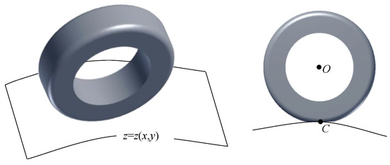
Figure 1.
An example of a sketch of the contact point position on the road surface.
According to the authors, locating this point is a complex task. When a vehicle moves over the road surface only a center position of a particular wheel is known (it results from geometrical parameters of a vehicle). The simplest way to find contact point is to assume that its coordinates are: , , . Such a situation is presented in Figure 2a.
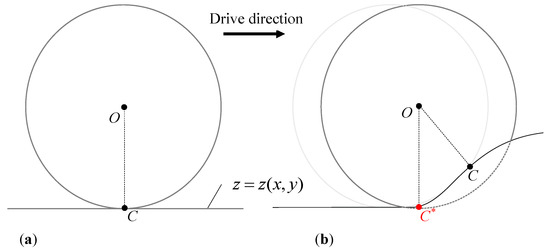
Figure 2.
An example of obtaining a contact point location on the road surface, (a) the flat road surface, (b) the uneven road surface.
As it can be seen, such a way of determining the contact point location is correct only when the vehicle wheels roll over the even area. This algorithm is not “sensitive” to area unevenness—this situation is presented in Figure 2b. The point marked , which results from the assumed procedure is not a proper point of contact of a wheel with the road surface. Therefore, in such a case the reaction forces acting on the vehicle wheels will interact at the wrong place. An appropriate algorithm of determining contact point should be sensitive to a changeable profile of the road surface in the surrounding of the moving wheel. It can be achieved by using four control points () in the surrounding of the point being the wheel center (point ), Figure 3.
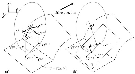
Figure 3.
A way of determining the contact point position in a precise way. (a) Stage 1—selecting the control points; (b) stage 2—determining contact point .
In the first stage projections of the control points selected on the road surface () are determined from the road surface equation. These points define versor being a normal vector of plane . Then, contact point is obtained as a point of straight-line (passed through point ) piercing ( with this plane. In such a way, a more precise procedure enabling the determination of the position of contact point C is presented in Figure 2. In paper [19] three proprietary algorithms presenting a precise position of contact point are presented jointly in detail; they are called: VectorCross, Plane, 4Point.
In the procedure described above, road surface equations must be known. The next chapter of this paper is devoted to this issue.
2. Road Surface Modeling
In case of the 3D graphic object shapes are often a set of line segments and curves which are edges of small flat planes (usually triangles), imperceptible to the eye (Figure 4).
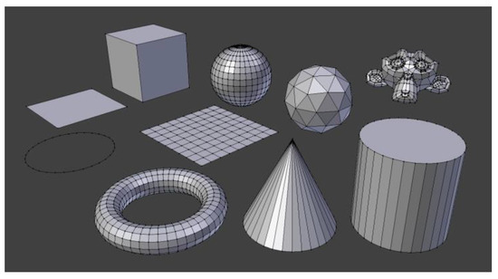
Figure 4.
An example of objects rendered using flat 2D objects (triangles, quads).
Following this idea, the authors have assumed that the road surface on which the vehicle moves is modeled using triangles (TIN surfaces). Some examples of the road surface modeled in such a way are presented in Figure 5.
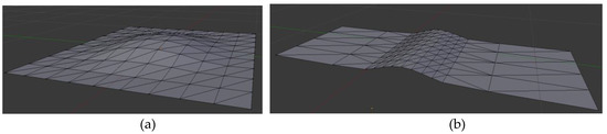
Figure 5.
Examples of objects divided into the triangles. (a) A sketch of a car roundabout; (b) a sketch of a speed bump.
It is worth noting (Figure 5b) that the road surface can consist of triangles of equal sizes. Generally, a number of triangles and their sizes are selected to represent the real shape of the road surface as accurately as possible.
The model of the surface can be defined as two sets:
- —a set of all points formulating the triangles.
- —a set of 3-element vectors defining all the triangles, that is , where are indexes of the points (from the set) being vertexes -th of this triangle. It means mathematically that for each element of the set a mapping function, which indicates that the element from the set describes a triangle of vertexes , was determined in a form of:
It is worth emphasizing that one element (a point) from the set can be a common element (a point) for two or more triangles simultaneously.
As it has been mentioned in the introduction, each algorithm of searching for contact point requires knowledge of coordinate for any point . Let this searching point be designated as where and are known whereas should be determined. Let point be in the area of the triangle of vertexes (Figure 6).
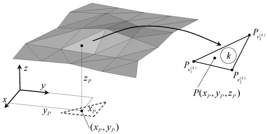
Figure 6.
Searched point .
The vertexes of this triangle determine the plane of which the normal equation has the following form:
where:
- are the elements of the versor normal to the triangle surface area,
- , where should be taken as any number from set .
Versor can be determined by the vector product:
where:
- —the vector with the beginning in point and the end in point ,
- —the vector with the beginning in point and the end in point .
Having the plane equation determined in (1), the searched coordinate of the point can be determined from the formula:
for , so excluding the situation when the triangle plane is perpendicular to the plane. In the described procedure, it has been assumed that the vertexes of the triangle, on which there is point P, are known. However, identification of this triangle is not a trivial task. It becomes especially difficult in a case of computer simulations where short time of calculations is usually significant. Therefore, it is essential to develop an appropriate algorithm of the triangle identification of the surface area in question.
2.1. Identyfying Surfce-Initial Stage
The trivial solution of the triangle identification problem consists of searching the whole set of triangles and checking if the searched element is in the surface area of this triangle. In this case, for each triangle () the plane Equation (1) should be determined, and it should be checked if the P point is in its fragment specified by vertexes . Such an algorithm does not belong to the efficient one regarding calculating, and because of three dimensionality it may prove to be problematic. Much better results can be obtained by reducing the problem to a two-dimensional issue and narrowing appropriately the set of the searched triangles. In this paper, the developed algorithm was divided into two stages.
2.1.1. Stage I—Reducing the Problem to a Two-Dimensional Issue
Let be a set of the points, with the projections of the points from the set on the plane. A two-dimensional (flat) map in which there are projections of the triangles of the area in question, is obtained in such a way. Then, a triangle is searched in this map; the triangle that consists of three appropriate points from set, (Figure 7).
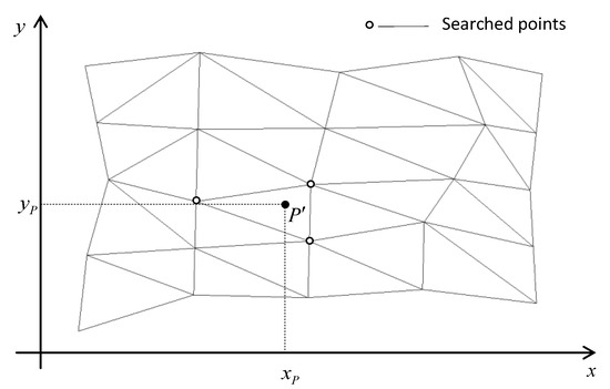
Figure 7.
Projection of the road surface area on the plane.
When the vertexes of this triangle are known, there are also known vertexes determining a position of a triangle corresponding to it in the three-dimensional space.
2.1.2. Stage II—Limiting the Search Set
A distance of a point from the point is determined by the formula:
Let be such a point of the set, of which the distance is the shortest. This point is called the nearest neighbor. Then, the hypothetical triangles, to which point may belong, are only those for which point is their common vertex, marked grey in Figure 8. There is a problem to find this point—a way of its searching can have a significant influence on the efficiency of the algorithm in question. A typical solution based on determining the distance (4) for all n points is not the optimal solution.
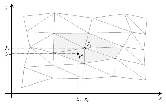
Figure 8.
Searched triangles (marked in grey).
2.2. Identyfying Surfce—An Efficient Algorithm
In this paper an effective algorithm based on the data structure of the kd-tree type was used to search the nearest neighbor [20]. The idea of this algorithm can be presented by using the following example. Let us have a set of 11 points () distributed as in Figure 9.
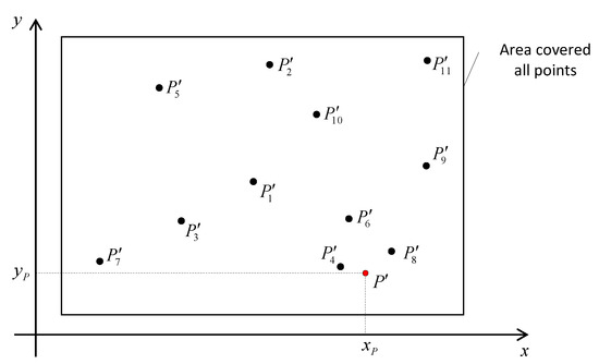
Figure 9.
Some examples of the point distribution, , are the point near which the point being its nearest “neighbor” is searched.
By appropriate cuts (decompositions) with vertical and horizontal planes [21] the area including the point is divided into rectangular sub-areas in order, as presented in Figure 10.
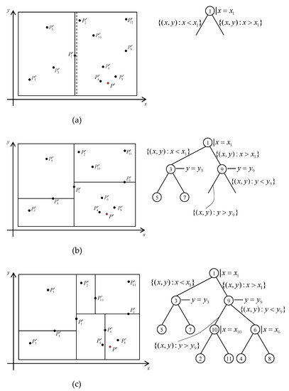
Figure 10.
The decomposition of the area of points using the kd-tree structure: (a) by plane , (b) by planes and , (c) by planes and .
The cutting plane is selected in an indirect way. For example, in order to make first cutting with the vertical plane, an auxiliary plane is determined which divides the area including all points into two equal sub-areas toward the axis (the dotted line in Figure 10a). Then, the target cutting plane goes through the point which is the nearest to the indirect plane, that is through point . Other cuttings are made in the same way, which is presented in the further part of the paper.
While decomposing the points belonging to particular sub-areas are collected in the binary tree. The root of this tree is point where the first cutting with plane was made (Figure 10a). As a result, the root branches determine the sub-areas (sets) of points, respectively: (a left branch) i (a right branch), where subsequent cuttings are made—horizontal in points 3 and 9 (Figure 10b), and then vertical in points 6 and 10 (Figure 10c). Cuttings are made until the specific sub-area contains one point at most. The nearest neighbor search (NNS) algorithm begins from the point (the node) which is in the same area as point . In order to find this point, it is enough to “walk” on the tree branches marked in blue (Figure 11). In the example in question, it is point .
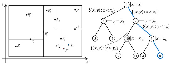
Figure 11.
A graphic presentation of the procedure of finding the point being in the same area as point .
A selection of the tree branches which must be “walked on” to find point , takes place by elimination. Starting from the root its right branch is selected due to the fact that . In two subsequent nodes their right branches are also selected, because and . Point is not the nearest neighbor of point (which can be seen in Figure 11). However, it is a point in the area which should be expected (from Figure 11 it results that the nearest neighbor is point ). In the next step, distance is calculated and a circle of center and radius is made (Figure 12). Then, the points being in the sub-areas with which the delineated circle intersects, are searched, (in Figure 12 these areas are marked in grey). It means you should “go” to the nodes with numbers: 6 (the parent of node no 8) and 4 (a child of node no 8) and calculate distances and . Finally, the shortest distance should be chosen among distances , and . In the example presented distance is the shortest one, therefore point is the solution to the NNS task.
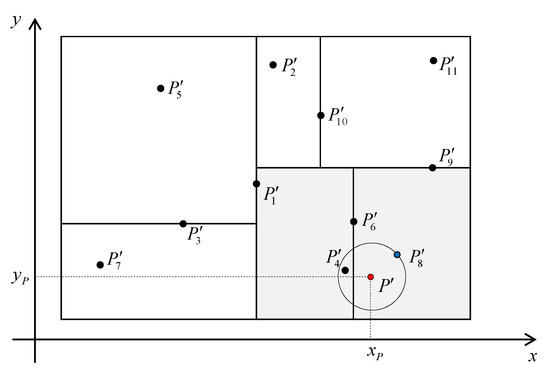
Figure 12.
A graphic presentation of the final stage of the procedure while using the kd-tree structure.
Use of the algorithm in question limits significantly a set of the searched points of set . As it has been shown in paper [22], in terms of efficiency the algorithm is classified into the algorithms of type , where is a number of points.
To sum up, the procedure of identifying an “appropriate” triangle of the surface area in question consists of certain steps that are specified in the diagram (Figure 13).
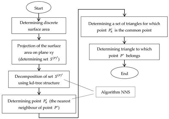
Figure 13.
Stages of triangle identification.
3. Road Reaction Forces Including Rolling Resistance
When a vehicle moves over the road surface, road reaction forces act on the vehicle wheels in contact point according to the sketch in Figure 14.
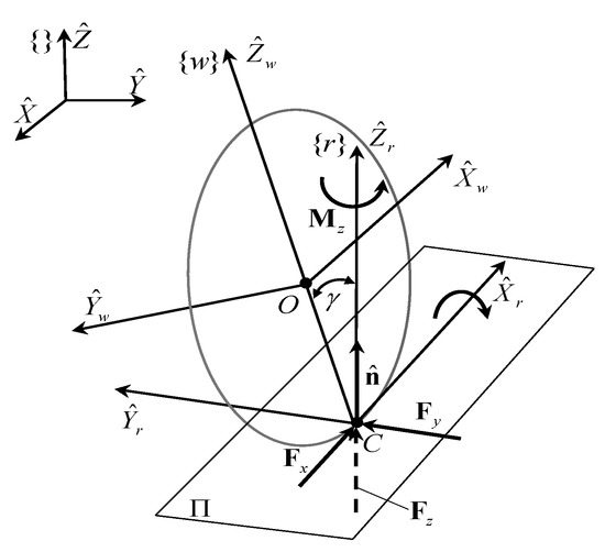
Figure 14.
Road surface reaction forces: —longitudinal force (rolling resistance), —lateral force, —aligning torque.
As it has already been mentioned in the introduction there are a lot of mathematical formulas called tire model which allow determining these forces. The Pacejka model of mathematical expressions determining the reaction forces known as “the Magic Formula” [3,4] was chosen for the purposes of this paper. The Pacejka’s Magic Formula tire models are widely used in professional vehicle dynamics simulations, and racing car games, as they are reasonably accurate, relatively easy to program, and solve quickly. This model is also well described on the Internet [23,24].
The mathematical formula has the form:
where:
and and are given in the further part of the paper. An approximate course of the function determined by relationships (5 and 6) is presented in Figure 15.
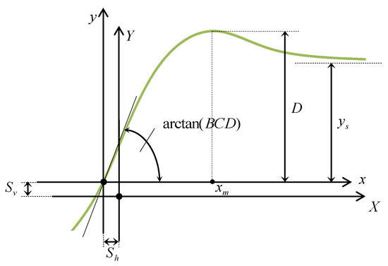
Figure 15.
A graphical presentation of Pacejka’s Magic Formula.
The maximum value of function is determined by parameter . Product enables to “control” the curve near the beginning of coordinate system .
For each of the reaction forces that is, longitudinal reaction force (rolling resistance) and lateral reaction force and the aligning torque , a separate set of coefficients is taken. These are the main coefficients that are determined on the basis of auxiliary coefficients:
The physical interpretation of the coefficients, being the elements of vectors , is characterized in papers [12,13]. On basis of these values the main coefficients and values and are determined according to the formulas:
Additionally, in (7) it can be assumed that: in the case of calculations of a component of the longitudinal reaction force , and in the case of calculations of components of the lateral reaction force and a value of the aligning torque. Values and are longitudinal tire slip and lateral tire slip angle, respectively, defined in many papers [8,9,11,23,24,25] and they are determined on the basis of calculations of vehicle dynamics.
4. Computer Simulations and Results
Two types of unevenness present frequently on the roads where speed limits of moving motor vehicles are introduced, were chosen for computer simulations, Figure 16.
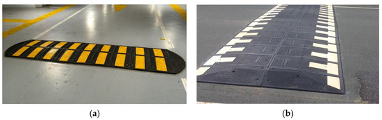
Figure 16.
Shapes of the profiles limiting speed of moving vehicles: (a) speed bump A, (b) speed bump B.
The shapes of these profiles, and precisely a course of a coordinate from the road surface profile, are presented in Figure 17—the first of them has a span of 1.4 m and the second 3 m, both are 0.06 m high.
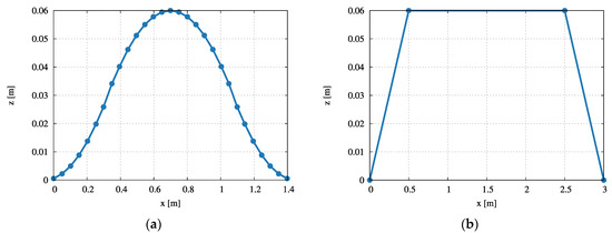
Figure 17.
Characteristic of the profiles selected, respectively for: (a) speed bump A, (b) speed bump B.
The dots presented in these diagrams symbolize points of the road surface division during its modeling in program Blender [26], Figure 18.
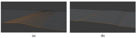
Figure 18.
The models of the profiles selected made in program Blender: (a) speed bump A, (b) speed bump B.
These models were made in two stages—first they were made by rectangles and then triangularization was performed. An example of profile B after triangularization is presented in Figure 19.
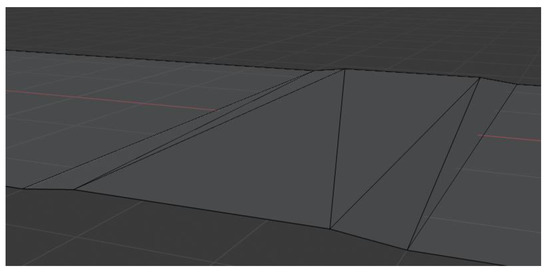
Figure 19.
Speed bump B after triangularization.
It has been assumed that a vehicle driving over the road surface unevenness is modeled in accordance with the sketch presented in Figure 20.
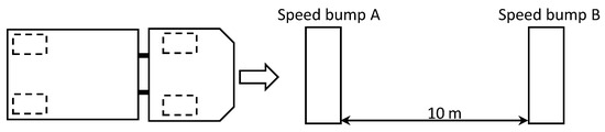
Figure 20.
A sketch presenting a computer simulation of driving over speed bumps.
The vehicle moved at a constant speed equal 15 km/h in 4 s. A detailed model of this vehicle with sub-components is presented in proprietary papers [19,25,27]. Proprietary software described in paper [28] was also used to perform the computer simulations. Coordinate of the contact point and rolling resistance force acting on the selected vehicle wheels were determined on the basis of the computer simulations—time courses of these values are presented in Figure 21.
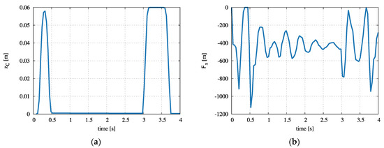
Figure 21.
Courses obtained as a result of the computer simulations: (a) a course of coordinate from contact point , (b) rolling resistance force .
As it can be seen, a course of coordinate (Figure 21a) of the contact point searched corresponds to the speed bump profiles. While driving onto the analyzed speed bumps, rolling resistance (Figure 21b) changes rapidly in the time intervals corresponding to the presence of unevenness. A comparison of courses of the rolling resistance force and a normal reaction of the road surface in relation to coordinate of the contact point is presented in Figure 22.
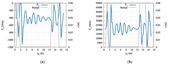
Figure 22.
The course of the road surface reaction with reference to the shape of the bumps: (a) rolling resistance force , (b) normal force .
As it can be seen in (Figure 22a) rolling resistance as to the absolute value increases while driving onto the speed bump and decreases while leaving the speed bump. Between the speed bumps it remains at the same level (oscillations result from suspension of a vehicle). The normal reaction force component behaves in a similar way (Figure 22b).
5. Discussion and Conclusions
A complete set of the methods that enable to make computer simulations of dynamics of vehicles moving over the uneven road surface is presented in the paper. The proprietary approach in a form of a set of elementary triangles forming TIN areas was used for modeling road surface unevenness. These triangles allow mapping precisely almost each road surface unevenness, except the situation described in Equation (3).
A free-of-charge tool that is the Blender graphic environment can be used to generate the road surface. It allows determining sizes of particular elementary triangles in any way.
The kd-tree algorithm, owing to which a task of dynamics can be made in a relatively short time, was implemented to optimize (speed up) locating control points. With a view to this fact, the proposed approach can be used in the tasks of optimization where computation time is critical.
The formulas determining the road surface reaction forces acting on vehicle wheels with additional interpretation are also presented in the paper. Although, these formulas are well-known in the literature they are rarely compiled comprehensively with the algorithms enabling to model the uneven surface.
In the works mentioned in introduction focusing on the movement of vehicles on uneven surfaces and in [29,30,31] the authors present in detail the selected road surface profile, modeled as an exact defined mathematical function. This function can be modelled based on the experimentally measured data of road profile [32] or this function can be applied arbitrarily as a known formula [33]. In some cases, analyses in this area are conducted based on a reduced car model with the road surface for a two-dimensional problem. Such a procedure is a certain simplification that allows to reduce the complexity of the mathematical model and the shortening of the computation time, and as a result, can be used in optimization problems [34]. Additionally, usually the procedure for determining the contact point is associated with a specific tire model. The main aim of the authors in this article was to create a universal mathematical methodology that would allow arbitrary modeling of the road surface on a macro scale, regardless of the tire model in three-dimensional space.
The presented procedure constitutes a compendium of knowledge needed to realize the task in question—not only dynamics of vehicles but other objects moving over the road surface with unevenness as well. The proposed approach can be used in the computer simulations of military equipment, robots, motorcycles. Cases that would be expensive and even impossible to be realized in the real-life conditions [35], can be simulated—for example in mentioned work three phases are highlighted, Figure 23a. The first one presets safe driving of the vehicle (green color), the second phase determines the initial loss of stability (orange color), and in the third phase the vehicle rollovers (red color). The example screenshots of this maneuver are presented in Figure 23b–d.
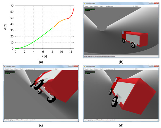
Figure 23.
The example of simulation of stability loss: (a) three phases of rollover maneuver, (b) beginning of computer simulation, (c) rollover started, (d) rollover.
The analyzed works of various authors show that the selection of the appropriate unevenness model and tire model depends on a specific case. In this article, the authors do not analyze the details of, for example, the structure of a suspension, which directly affects the comfort of driving, but rather the formulation of a mathematical algorithm which allows to conduct simulations of the dynamics of various objects moving on an uneven road surface in a short calculations time. The elaborated algorithm allows for conducting numerous computer simulations of road maneuvers, which can most often be observed on roads in real conditions, including: the optimization process, issues related to the improvement of the driver’s comfort, and stability loss of vehicle. The mentioned above areas are already the subject of authors’ research [36,37,38,39,40].
Real driving tests are also the subject of authors’ research, Figure 24a. They allow to verify the discussed calculation algorithm for computer simulations of vehicles dynamics on an uneven road surface, Figure 24b. Additionally, the systematic development of software for engineering calculations and visualization of vehicle motion is in progress [41].
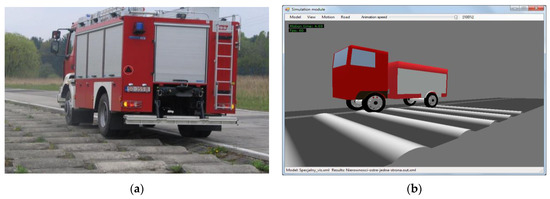
Figure 24.
The examples of road tests with computer simulation performed by authors: (a) experimental tests, (b) computer simulations.
The presented procedure constitutes a compendium of knowledge needed to realize the task in question—not only vehicles dynamics but also other objects moving over the area with unevenness. The proposed approach can be used in the computer simulations of military equipment, robots, motorcycles. Cases that would be expensive and even impossible to be realized in the real-life conditions, can be simulated.
The subject of the authors’ future works will be introducing a map which will allow generating areas with different rolling resistance values. This will allow conducting interesting computer simulations and formulate further conclusions.
Author Contributions
Conceptualization, S.T. and K.W.; methodology, S.T.; software, S.T. and K.W.; validation, S.T.; formal analysis, S.T.; editing, S.T.; visualization, S.T. All authors have read and agreed to the published version of the manuscript.
Funding
This research received no external funding.
Conflicts of Interest
The authors declare no conflict of interest.
References
- Mastinu, G.; Ploechl, M. Road and Off-Road Vehicle System Dynamics Handbook; CRC Press: Boca Raton, FL, USA, 2017. [Google Scholar]
- Sebsadji, Y.; Glaser, S.; Mammar, S.; Netto, M. Vehicle Roll and Road Bank Angles Estimation. IFAC Proc. Vol. 2008, 41, 7091–7097. [Google Scholar] [CrossRef]
- Öijer, F.; Edlund, S. 17th International Association for Vehicle System Dynamics-Complete Vehicle Durability Assessments Using Discrete Sets of Random Roads and Transient Obstacles Based of Q-distribution. In The Dynamics of Vehicles on Roads and on Tracks; Taylor & Francis: Oxfordshire, UK, 2016; pp. 67–74, Published online. [Google Scholar] [CrossRef]
- Lozia, Z. An analysis of vehicle behaviour during lane-change manoeuvre on an uneven road surface. In Supplement to Vehicle System Dynamics; Swets & Zeitlinger B. V. Lisse and IAVSD: Lisse, The Netherlands, 1992; Volume 20, pp. 417–443, Published online. [Google Scholar]
- Bogsjö, K.; Podgórski, K.; Rychlik, I. Models for road surface roughness. Veh. Syst. Dyn. 2012, 50, 725–747. [Google Scholar] [CrossRef]
- Kropáč, O.; Múčka, P. Effect of obstacles in the road profile on the dynamic response of a vehicle. Proc. Inst. Mech. Eng. Part D J. Automob. Eng. 2008, 222, 353–370. [Google Scholar] [CrossRef]
- Múčka, P. Influence of road profile obstacles on road unevenness indicators. Road Mater. Pavement Des. 2013, 14, 689–702. [Google Scholar] [CrossRef]
- Fiala, E. Leteral Forces at the Rolling Pneumatic Tire; Technische Hochschule: Wien, Austria, 1954. [Google Scholar]
- Dugoff, H.; Fancher, P.; Segel, L. An Analysis of Tire Traction Properties and Their Influence on Vehicle Dynamics Performance. SAE Tech. Pap. 1970, 1219–1243. [Google Scholar]
- Uffelmann, F. Rechenmodell Eines Reifens fur Seiten und Umfangskraftubertragung; VDI-Verlag, Institut für Fahrzeugtechnik Braunschweig: Braunschweig, Germany, 1989. [Google Scholar]
- Pacejka, H.B. Tyre and Vehicle Dynamics; Delft University of Technology: Delft, The Netherland, 2002. [Google Scholar]
- Pacejka, H.B.; Bakker, E. The Magic Formula Tyre Model. Veh. Syst. Dyn. 1993, 21, 1–18. [Google Scholar] [CrossRef]
- MSC.ADAMS Using ADAMS/Tire Tire Models. Available online: https://simcompanion.mscsoftware.com/infocenter/index?page=content&id=DOC9310, (accessed on 23 March 2021).
- Hirschberg, W.; Rill, G.; Weinfurter, H. User-Appropriate Tyre-Modelling for Vehicle Dynamics in Standard and Limit Situations. Veh. Syst. Dyn. 2002, 38, 103–125. [Google Scholar] [CrossRef]
- Gipser, M. FTire, a New Fast Tire Model for Ride Comfort Simulations; COSIN Software; Germany, Esslingen University of Applied Sciences: Esslingen am Neckar, Germany, 2007. [Google Scholar]
- Rafei, M.; Ghoreishy, M.H.R.; Naderi, G. Computer simulation of tire rolling resistance using finite element method: Effect of linear and nonlinear viscoelastic models. Proc. Inst. Mech. Eng. Part D J. Automob. Eng. 2019, 233, 2746–2760. [Google Scholar] [CrossRef]
- Gudsoorkar, U.; Bindu, R. FEM for Modeling and Analysis of Retreaded Tire with Abaqus Software. In CRRM 2019—System Reliability, Quality Control, Safety, Maintenance and Management; Springer: Singapore, 2020; pp. 92–97. [Google Scholar]
- Zhang, Y.; Gao, J.; Li, Q. Study on tire-ice traction using a combined neural network and secondary development finite element modeling method. Concurr. Comput. Pr. Exp. 2019, 31, e5045. [Google Scholar] [CrossRef]
- Tengler, S.; Harlecki, A. Determination of the position of the contact point of a tire model with an uneven road surface for purposes of vehicle dynamical analysis. J. Theor. Appl. Mech. 2017, 55, 3. [Google Scholar] [CrossRef][Green Version]
- Brown, R.A. Building a Balanced k-d Tree in O(kn log n) Time. J. Comput. Graph. Tech. (JCGT) 2015, 4, 50–68. [Google Scholar]
- Wald, I.; Havran, V. On building fast kd-Trees for Ray Tracing, and on doing that in O(N log N). In Proceedings of the 2006 IEEE Symposium on Interactive Ray Tracing, Salt Lake City, UT, USA, 18–20 September 2006; pp. 61–69. [Google Scholar] [CrossRef]
- Lee, D.T.; Wong, C.K. Worst-case analysis for region and partial region searches in multidimensional binary search trees and balanced quad trees. Acta Inform. 1977, 9, 23–29. [Google Scholar] [CrossRef]
- Tire Model for Longitudinal Forces. Available online: https://x-engineer.org/automotive-engineering/chassis/vehicle-dynamics/tire-model-for-longitudinal-forces/ (accessed on 23 March 2021).
- Tire-Road Interaction (Magic Formula). Available online: https://uk.mathworks.com/help/physmod/sdl/ref/tireroadinteractionmagicformula.html (accessed on 23 March 2021).
- Tengler, S. Analysis of Dynamics of Special Vehicles with High Gravity Center (in Polish). Ph.D. Thesis, Faculty of Mechanical Engineerim and Computer Science, University of Bielsko-Biala, Bielsko-Biała, Poland, 2012. [Google Scholar]
- Blender Free 3D Graphical Software. Available online: https://www.blender.org/ (accessed on 23 March 2021).
- Warwas, S.; Tengler, S. A hybrid optimization method to improve driver’s comfort. In Proceedings of the 2017 IEEE International Conference on INnovations in Intelligent SysTems and Applications (INISTA), Gdynia, Poland, 3–5 July 2017. [Google Scholar] [CrossRef]
- Tengler, S.; Harlecki, A. Computer program for dynamic analysis of special vehicles with high gravity centre. Tech. Trans. 2015, 2, 291–299. [Google Scholar]
- Alcazar, M.; Perez, J.; Mata, J.E.; Cabrera, J.A.; Castillo, J.J. Motorcycle final drive geometry optimization on uneven roads. Mech. Mach. Theory 2020, 144, 103647. [Google Scholar] [CrossRef]
- Limebeer, D.J.N.; Sharp, R.S.; Evangelou, S. Motorcycle steering oscillations due to road profiling, Trans. ASME J. Appl. Mech. 2002, 69, 724–739. [Google Scholar] [CrossRef][Green Version]
- Rill, G.; Kessing, N.; Lange, O.; Meier, J. Leaf spring modeling for real time applications. In The Dynamics of Vehicles on Road and on Tracks–Extensive Summaries; IAVSD 03; Atsugi: Kanagawa, Japan, 2003. [Google Scholar]
- Krauze, P.; Kasprzyk, J. Driving Safety Improved with Control of Magnetorheological Dampers in Vehicle Suspension. Appl. Sci. 2020, 10, 8892. [Google Scholar] [CrossRef]
- Jacobson, B.J.H. Vehicle Dynamics Compendium; Chalmers University of Technology: Gothenburg, Sweden, 2019. [Google Scholar]
- Kim, S.; Nikravesh, P.E.; Gim, G. A two-dimensional tire model on uneven roads for vehicle dynamic simulation. Veh. Syst. Dyn. 2008, 46, 913–930. [Google Scholar] [CrossRef]
- Tengler, S.; Harlecki, A. Analysis of dynamics of special vehicles with high gravity centre-the case of stability loss. Int. J. Appl. Mech. Eng. 2012, 17, 1003–1011. [Google Scholar]
- Warwas, K.; Tengler, S. Dynamic Optimization of Multibody System Using Multithread Calculations and a Modification of Variable Metric Method. J. Comput. Nonlinear Dyn. 2017, 12, 051031. [Google Scholar] [CrossRef]
- Tengler, S.; Warwas, K. Driver comfort improvement by a selection of optimal springing of a seat. Tech. Trans. 2017, 5, 217–235. [Google Scholar] [CrossRef]
- Tengler, S.; Warwas, K. Increase Driver’s Comfort Using Multi-population Evolutionary Algorithm. In Recent Challenges in Intelligent Information and Database Systems; ACIIDS 2021. Communications in Computer and Information Science; Hong, T.P., Wojtkiewicz, K., Chawuthai, R., Sitek, P., Eds.; Springer: Singapore, 2021; Volume 1371. [Google Scholar] [CrossRef]
- Tengler, S.; Warwas, K. Distributed Multi-Population Genetic Algorithm to improve driver’s comfort. In Proceedings of the 14th International Conference on Dynamical Systems-Theory and Applications Engineering Dynamics and Life Sciences, Łódź, Poland, 11–14 December 2017; pp. 541–552. [Google Scholar]
- Warwas, K.; Tengler, S. Multi-Population Genetic Algorithm with the Actor Model Approach to Determine Optimal Braking Torques of the Articulated Vehicle; Computing Conference, Springer series Advances in Intelligent Systems and Computing; Springer: Metro Manila, Philippines, 2021; in press. [Google Scholar]
- Warwas, K.; Tengler, S. Computer program for the simulation of physical structures based on the joint co-ordinates and homogenous transformations. In Proceedings of the 7th Conference on Computer Methods and Systems, Krakow, Poland, 26–27 November 2009; pp. 447–452. [Google Scholar]


Publisher’s Note: MDPI stays neutral with regard to jurisdictional claims in published maps and institutional affiliations. |
© 2021 by the authors. Licensee MDPI, Basel, Switzerland. This article is an open access article distributed under the terms and conditions of the Creative Commons Attribution (CC BY) license (https://creativecommons.org/licenses/by/4.0/).