Affinity between Bitumen and Aggregate in Hot Mix Asphalt by Hyperspectral Imaging and Digital Picture Analysis

Abstract

This study investigated the viability of quantifying the affinity between aggregate and bitumen by means of different imaging techniques. Experiments were arranged in accordance with the rolling-bottle test, as indicated in UNI EN 12697-11, “Test methods for hot bituminous conglomerates—Part 11”. Digital image processing (DIP) techniques have only recently been used for such quantification. The data gathered with a multi-sensor optical platform equipped with VIS–NIR and SWIR spectrometers were compared with DIP outcomes. Data were processed using the unsupervised ISODATA and the supervised parallelepiped algorithms. The exposed aggregate index (EAI) and the bitumen index (BIT) were calculated to retrieve the bitumen percentage coverage of different mixtures. The comparison with the results obtained employing the traditional 6, 24, 48 and 72 testing hours reveals the possibility to implement a standardized analysis methodology combining digital and hyperspectral imagery to highlight potential inaccuracies deriving from the visual interpretation.

1. Introduction

Hot mix asphalts (HMAs) of road pavements are composed of different combinations of aggregates and bituminous binders. Aggregates can vary depending on their origin (natural, artificial, and recycled), lithology (usually constituted by SiO₂, CaO, and MgO), and size [1]. From the physical point of view, bitumen gives rise to a multi-phase system characterized by asphaltenes, resins, and oil. The asphaltenes are largely responsible for the behavior of bitumen as a viscous body with plasticity and elasticity. The resins confer flexibility and are important for interfacial adhesion and ductility of the flooring [2]. The malthenes represent the fluid bituminous components, which are essentially composed of carbon (80–87%), hydrogen (9–11%), oxygen (2–8%), nitrogen, sulfur compounds and trace metals (0–1%) [3]. Different factors determine the response and behavior of an asphalt, including the temperature and loading time. The compound is liquid or solid at high or low temperatures, respectively. This property of asphalt as a pavement causes it to crack at low temperatures or suffer rutting at high temperatures. Factors such as oxygen, ultraviolet (UV) sunlight, and heat affect both the physical properties and the asphalt chemical structure and cause the phenomenon called aging [4]. Another antagonist of the asphalt binder is moisture. The moisture damage of asphalt mixtures is defined as the progressive loss of functionality of the material due to a drop of the adhesive bond between the asphalt binder and the aggregate surface. The premature deterioration of asphalt pavements caused by moisture in asphalt mixtures is related to stripping, raveling, and hydraulic scour [5].

The adhesion between bituminous mixtures’ constituents is essential for the endurance of an asphalt pavement [6]. For these reasons, specific laboratory analyses are available to quantify the affinity between aggregate and bitumen. In particular, the European Standard EN 12697-11 methodology [7], “Bituminous mixtures—Test methods for hot mix asphalt—Part 11”, specifies procedures for the determination of the affinity between aggregate and bitumen and its influence on the susceptibility of the combination to stripping. The susceptibility to stripping is an indirect measure of the power of a binder to adhere to various aggregates, or vice versa [7]. The control method provided by the affinity tests according to the methodology [7] is included in the standard tender documents for procurement of roads works, becoming a prescriptive method between client and supplier for the use of certain aggregates in road constructions.

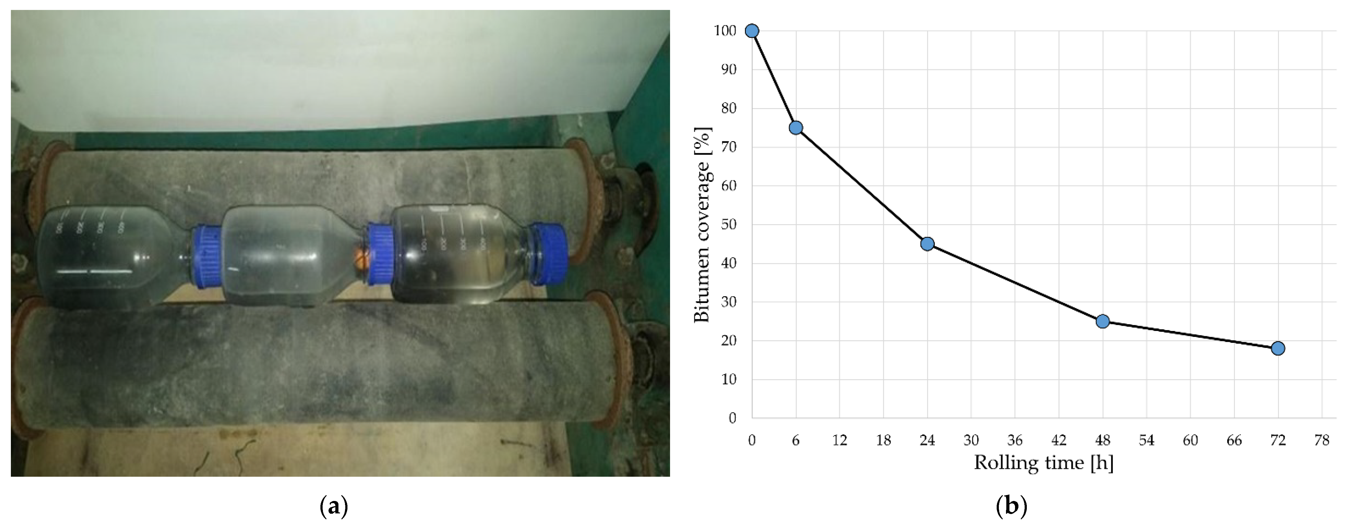
The most widely used standard procedures are the rolling-bottle test, the static test, and the boiling water stripping test. In the rolling-bottle test, the affinity is expressed as the degree of bitumen coverage on uncompacted bitumen-coated mineral aggregate particles after the influence of a mechanical stirring action in the presence of water. In the static test, affinity is measured in terms of the degree of bitumen coverage on uncompacted bitumen-coated mineral aggregate particles after storage in water. For both tests, affinity is determined by the operator via visual inspection. As mentioned in the standard specifications, the rolling-bottle test and the static test are simple and suitable for routine testing and for high polished stone value aggregates. The shortcoming is that they are subjective. Furthermore, the static test is generally less precise. In the boiling water stripping test, the affinity is expressed by determining the degree of bitumen-coverage on uncompacted bitumen-coated aggregates after immersion in water under specific conditions. The boiling water stripping test is an objective test characterized by high precision. However, it requires greater operator skills compared to the other tests, and, because of its use of chemicals as reagents, extra safety requirements must be employed [7]. For its simplicity, the rolling-bottle test is the most used procedure.

Recent advancements in spectrometry and digital imaging processing (DIP) techniques can make it possible to overcome the subjectivity of the rolling-bottle test. In the literature, different ways to detect chemical and physical properties of bituminous mixtures can be found and, specifically, the use of different techniques to quantify the degree of bitumen’s aggregate coverage are described. As is known, due to both natural and artificial degradation processes, bituminous mixtures lose superficial bitumen, and the exposure of the aggregate compounds modifies their spectral response [8,9]. The absorption of silicates and hydrocarbons affects the short-wave infrared (SWIR) region, especially at 1750 nm and after 2100 nm [10,11], while bitumen loss causes a slope change in the visible (VIS) region [12]. The use of spectroscopy can be helpful in quantifying bitumen removal on aggregate surfaces. For this reason, several studies have focused on the adoption of imaging techniques to objectivize the bitumen removal on them. Recently, spectroscopy and DIP techniques have been employed for bituminous mixtures analysis in both field and laboratory environments. In [13], the bitumen coverage of asphalt mixture surfaces is retrieved using the 2D distribution of remote sensing data via the asphalt-line computation. At the same time, digital pictures are employed to quantify bituminous pavement cover using the geologic classification of Shvetsov (1954) [14].

In recent years, DIP has been widely used in engineering studies to retrieve some physical parameters in unbiased and fast ways. In engineering, this kind of analysis is promising for the detection of the morphometric characteristics of aggregates in both loose and specimen forms [15] and in the reconstruction of grain size curves starting from specimens [16] or thin sections [17]. Images are used to retrieve parameters related to the road macro-texture by road surface modeling [16,18] for calculating the binder/aggregate ratio and grading curve retrieval by digital imaging segmentation [17] or aggregates’ characterization [15]. Different authors focused on the application of DIP for bitumen removal using field and laboratory samples. As shown in [19,20], spectral data and DIP of bituminous mixtures make it possible to find a spectral model for the objective quantification of superficial bitumen removal. This analysis is performed by the computation of the exposed aggregate index (EAI). Considering that the brightness of new asphalt is lower than that of older ones, spoliation effects can be linked to colorimetric variation in the visible range, and a sensitivity analysis of the tested model demonstrates the robustness of the identified relation.

Two semi-automatic methods that reliably replace the subjective assessment are presented in [21,22]. The first one is based on gray level thresholding (GLT), while the second one on entropy-based image segmentation (EIS). The GLT method is adopted to recognize brightness and shadows on the digital image of asphalt mixtures, while the EIS method is used to assess the roughness of the texture.

According to the authors of [23], the computerized analysis technique is based on the digital representation of the bitumen–aggregate system after the lamination process and the classification of the characteristic color zones by means of commercial software. As a side effect, there is a reduction in the labor required for the test analysis. The bituminous coverage of the stones using two different methods of digital image analysis is evaluated in [24]. This method works for stones of any color because bitumen reflects light much better than rough stones.

A 2D image analysis is employed to evaluate the results of the rolling-bottle test in [25]. To demonstrate its applicability to a wide range of materials, this procedure is applied to both light and dark aggregates, mixed with a wax-modified binder. The mixing temperature is varied to evaluate the influence of the binder’s viscosity on adhesion. Visual and semi-automatic estimations are compared through confusion matrices, and it is demonstrated that the proposed method leads to far better results. In [26], the degree of coverage of bitumen is measured with digital image processing methods by using a professional camera and an ordinary smartphone. Image J is used to process images.

In [27], a vision-based algorithm and a low-cost light enhancement system is developed as an alternative to visual inspection. The system processes images of samples captured under a controlled lighting condition and then applies contrast-limited adaptive histogram equalization to enhance the contrast intensity of the image. In addition, the system uses inpainting to reconstruct the specular highlights in the image, and then classifies the regions on the image, i.e., the coated and stripped areas, using combinations of K-means clustering, K-nearest neighbors, and support vector machines classifiers.

Fourier transform infrared (FTIR) has also been used to achieve this result. In [28], the bitumen overlay of aggregates with reference to FTIR microscopy in attenuated total reflectance (ATR) mode is investigated. This method is a promising alternative to trace heterogeneous areas within the coating compared to methods that require extraction and recovery of the bitumen. In [29], several types of mineral aggregates are characterized in detail by optical microscopy and X-ray powder diffraction in order to investigate the potentiality of the boiling test and the contact angle method to detect the level of bitumen/aggregate affinity.

The above-mentioned techniques show that DIP and some other imaging techniques represent useful tools to quantify the bitumen coverage of several aggregates. In this study, VIS–NIR and SWIR imaging spectrometers and a high-resolution digital camera were set in a multi-sensor platform to investigate their potentiality for bitumen removal quantification. A hyperspectral system has been employed in different applications such as the identification of vegetation diseases [30,31], the detection of marine plastic litters [32], and plastics separation [33,34]. Different approaches were investigated to extrapolate the degree of bitumen coverage in the rolling-bottle test at 6, 24, 48 and 72 h. To achieve this goal, samples of trachytic and limestone mixtures were tested at different temporal steps with supervised (parallelepiped) and unsupervised (iterative self-organizing data analysis technique (ISODATA)) algorithms and finally compared with several operators’ visual observations.

Remarkably, by comparing the different techniques, this study demonstrated that, by means of both VIS–NIR and SWIR spectrometers and a digital camera, an objective quantification of the bitumen loss caused by the stripping process can be obtained and inaccuracies related to visual inspection overcome.

2. Materials and Methods

2.1. Mix-Design

To maintain the physical/chemical properties of the binder, only 50/70 Repsol^® bitumen was used in this research work. Some of the physical properties of the bitumen are shown in

Table 1. Some of the physical properties of the bitumen used.

Characteristics	Unit	50/70	UNI EN
Penetration at 25 °C	0.1 mm	50–70	1426
Softening point	°C	46–54	1427
Penetration ratio	-	from −1.5 to +0.7	12591
Fraass breaking point	°C	≤−8	12593
Flash point in open cup	°C	≥230	ISO 2592
Solubility	%	≥99.0	12592

.

In this research, two different kinds of aggregates were used. The first one is a light aggregate of trachytic nature. This product was obtained by crushing trachytic rock from the quarry in Montalto di Castro (Italy). The second one is a micritic limestone. After mining, the limestone rock was subjected to a process of crushing with the formation of aggregates of various particle sizes. This product came from Campiglia Marittima (Italy).

Table 2. The average chemical composition of the selected aggregates.

Characteristics	Unit	Trachytic	Limestone
Sulphates Content	%	0.0068	0.017
Chlorides Content	%	0.0016	-
Acid-soluble sulphates	%	<0.9	-
Total sulfur	%	0.088	-
Dangerous substances	-	N.P.	N.P.

shows the average chemical composition of the two selected aggregates.

2.2. The Rolling-Bottle Test

The degree of bitumen adhesion to aggregates influences the mechanical performance of an HMA. The UNI EN 12697-11 methodology [7] specifies the procedures for determining the affinity between aggregate and bitumen according to three different approaches: the rolling-bottle, static, and boiling tests. As mentioned in the Introduction, the standard specifications indicate the rolling-bottle test as the simplest and most widely used method for the routine testing of high polished stone value aggregates. For such features, this method was chosen for carrying out this research. First, the bitumen and aggregate affinity was evaluated via visual inspection after mechanical agitation in water. The equipment required a bottle-rolling device able to rotate 3 Pyrex test bottles (diameter equal to 86 mm and height equal to 176 mm) at a specified speed within 40 and 60 min⁻¹ (Figure 1).

The standard includes three different preparatory stages through which aggregates and bitumen are prepared and conditioning parameters set. As regards the preparatory stage of the aggregates, this involves granulometric analysis to separate at least 600 g of aggregate through 11.2 and 8 mm sieves to produce, as defined in EN 12697-2 [35], a fraction to be tested between 8 and 11 mm. The resulting aggregates are rinsed and then placed in an oven at 110 ± 5 °C until a stable mass value is reached. In a mixer, a quantity of 510 ± 2 g of aggregates is introduced, which is mixed with 16 ± 0.2 g of bitumen, until a bitumen aggregate is achieved in accordance with EN 12697-35 [36]. The conditioning stage initially involves a period between 12 and 64 h at an ambient temperature of 20 ± 5 °C, avoiding direct exposure to sunlight and contamination with dust. After this period, the material is fractionated into three parts of 150 ± 2 g each and placed into three Pyrex bottles filled to about 50% of the volume with distilled water at a temperature of about 5 ± 2 °C. To reduce adhesion between the aggregates, the mixture is shaken.

The procedure is carried out by rotating the bottles at a controlled speed of 40 RPM. The rotation times are 6 h ± 15 min, 24 h ± 15 min, 48 ± 1 h and 72 ± 1 h. To optimize the visual inspection, samples are positioned above a plastic paper and put in an obscured and sterile camera to avoid exposure to sunlight and dust contamination. According to a reference procedure [7], to estimate the degree of bitumen coverage, after the mixtures are rinsed, samples are analyzed by visual inspection performed by at least two different observers.

Although the standard procedure imposes a very detailed scheme with different steps, some uncertainty elements may be encountered that may affect the reproducibility of the inspection and the repeatability of the analyses. These issues are summarized in the following points:

• The standard prescribes the estimation of the degree of bitumen coverage employing only a few values, i.e., 100%, 95%, 90%, 80%, 60%, 40%, and 20%, without any prescription about intermediate percentage readings.
• Difficulty in extrapolating the percentage of bitumen coverage may arise depending on the type of aggregates due to the influence of their color and brightness. This difficulty is accentuated in the case of dark aggregates where the difference between aggregate and bitumen is less easy to detect.
• There is no official procedure for calculating the accuracy of the observations.

As regards Points 2 and 3, such aspects are explicitly reported within the standard. Considering that the adhesion capacity of bitumen to aggregates affects the occurrence of phenomena such as cracking, it is crucial to define new analytical methods that can overcome the mentioned challenges.

2.3. The Multi-Sensor Platform

The multi-sensor platform consists of three units suitable for the acquisition of data with different dimensionality and spectral domains, ranging from visible to short-wave infrared. The platform includes a hyperspectral device equipped with VIS–NIR (Specim, Spectral Imaging LTD., Oulu, Finland) and SWIR (2D information in the spectral range 400–1700 nm, Specim, Spectral Imaging LTD., Oulu, Finland) spectrometers imaging systems and a high-resolution digital camera that captures true color images (2D information). Each sample to be analyzed is placed on a sampler mounted on a conveyor belt, which, by moving, places the object under investigation below the various sensors. The sampler consists of a slab featuring black and white metric references, useful for the geometric correction of the image. The lighting system was optimized to provide an appropriate amount of light for each instrument. Figure 2 shows the multi-sensor platform devices, the conveyor belt arranged in the aluminum structure holding the VIS–NIR and SWIR spectrometers’ imaging system, and the laptop employed to store the data. All measurements were performed using two halogen lamps which feature a bidirectional light to minimize shadow effects during measurements in laboratory.

2.3.1. Digital Camera

DIP is used in a wide area of environmental and engineering studies where processing techniques are carried out to quantify characteristics and quantities that would otherwise be difficult to obtain. In addition, the application of methodologies other than the classical engineering tests, such as those prescribed by UNI EN 12697-11 [7], is of great interest if they are non-destructive and semi-automatic. A digital camera was added to the multi-sensor platform to quantify the surface percentage of exposed aggregates using only RGB values. A NIKON D7000 digital camera (Nikon, Tokyo, Japan) was used for image acquisition. The camera features a 23.6 × 15.6 mm² CMOS sensor which allows the acquisition of 4928 × 3264 pixels (16.9 million pixels) images, a 12-bit NEF (RAW) capture format, and a lens with 18–50 mm focal length range. The camera was placed at a height of about 50 cm. An initial pre-processing step allowed co-registering the dataset and standardize the area of interest (AOI). The AOI comprises 743 rows and 761 columns (565,423 pixels) to ensure that the ground instantaneous field of view (GIFOV) of the spectrometers is within the area. For each sample, a digital picture was taken in the same lighting condition geometry. By using a white reference, a pre-calibration of each image was performed to standardize the dataset.

2.3.2. VIS–NIR and SWIR Imaging Spectrometers

The hyperspectral imaging system consisted of an integrated hardware and software architecture able to digitally capture and handle spectral attributes of each pixel in an image. Thus, it was possible to acquire hyperspectral images, namely hypercubes, i.e., a three-dimensional dataset with two spatial dimensions and one spectral dimension. The cores of such a device are the spectrometers. The first one collected spectral data in the visible/near-infrared (VIS–NIR) range of the electromagnetic spectrum (400–1000 nm), while the second spectrometer operated in the short-wave infrared region (SWIR) (900–1700 nm). Each spectrometer captures a line image of a target and disperses the light from each line image pixel into a spectrum. Each spectral image thus contains line pixels in a spatial axis and spectral pixels in a spectral axis. A 2D spectral image sequence can be formed by sequentially acquiring images of a moving target or by moving the push broom spectral device.

Figure 2 shows a diagram of the system configuration, comprising one VIS Specim Imspector spectrometer (S1, Specim, Spectral Imaging LTD., Oulu, Finland) mounted in front of a Dalsa 4M60 CMOS camera (2352 × 1728 pixels @ 25 fps, spectral resolution up to 3 nm, Teledyne DALSA, Waterloo, ON, Canada); one NIR Specim Imspector spectrometer (S2, SPECIM, SPECTRAL IMAGING LTD., Oulu, Finland), mounted in front of a Xeva Xenics InGaAS camera (640 × 512 pixels @ 25 fps, spectral resolution up to 3 nm, Xenics, Leuven, Belgium); one Dalsa 4M60 CMOS camera (2352 × 1728 pixels @ 25 fps), equipped with a standard lens, for image mosaicking and georeferencing of the lines acquired by the spectrometers; one high-speed DVR CORE (frame grabber) with three camera link inputs (IO Industries DVR Express^® Blade, London, ON, Canada) used to trigger camera acquisition and manage the data acquisition and image storage on the 1-TB solid state disk array; one power supply for all system devices; one processing computer for controlling the entire system and acquiring images; one lighting system comprising two 250 Watt halogen lamps; and one conveyor belt to allow maintaining the target displacement at a constant rate.

The spectral devices and camera equipped with standard lens simultaneously acquired images at a rate of 25 frames per second. The synchronization signal was generated by the frame grabber.

The characterization of materials via the hyperspectral imaging system required the following steps.

The geometric correction is the first step to create the single images forming the hyperspectral cube. Since the samples are placed on a conveyor belt moving at a constant speed in a fixed direction, the reconstruction of the images at the various wavelengths is performed by simply placing side-by-side rows of the acquired image sequence. This implies the slit of the spectrometer is set perpendicular to the direction of movement of the object and the device collimation axis normal to the conveyor belt plane. Vignetting effects are eliminated from each image. This imperfection causes the reduction of brightness at image edges with respect to its center. Noise filtering is further considered. The CMOS and InGaAs arrays employed for image acquisitions are subject to various sources of noise, including thermal noise, shot noise, and electronic noise in the amplified circuitry. To reduce noise effects, images are convolved with a Gaussian mask.

The radiometric calibration constitutes one of the most sensitive pre-processing steps since it ensures the construction of a spectral library as close as possible to the material characteristics. This is achieved by eliminating the dependence on the spectra of the measuring instruments. In fact, the acquisition system does not record the material reflectance but rather the value of radiance, i.e., the part of the reflected radiation that reaches the camera sensor with energy content sufficient to be recorded. The absolute reflectance of the materials can be calculated only if the incident radiation on the target is known. The relative reflectance is then calculated. This is achieved by comparison with a reference spectrum chosen ad hoc. The flat field (FF) method requires the presence of targets with smooth reference reflectance spectrum. We employed this method by introducing in the scene a white reference standard. A high-density fluoropolymer panel (Spectralon, Labsphere, NH, USA), assumed to be a Lambertian surface, was used as the white reference to retrieve spectral signatures on reflectance values.

The extraction of spectral signatures was performed on the spectrally and radiometrically calibrated hyperspectral cube to produce an image in which pixels with similar spectral signatures are associated with the same class. This allows defining a spectral library or set of reference spectra. Through the analysis of the spectra, it is possible to recognize and then classify the different materials.

2.4. Algorithms

The platform was composed of three instruments which are characterized by distinct spectral and spatial resolutions. For the analysis of digital pictures and hyperspectral data, two distinct techniques were adopted. The ISODATA unsupervised and the parallelepiped supervised classification methods were employed for image classification. The trend of the bitumen coverage loss obtained by such different techniques was calculated and then compared with visual inspection evaluations, as indicated in UNI EN 12697-11 [7].

The unsupervised method does not require a training dataset to perform classification, while the supervised method needs the generation of representative region of interest (ROI) files. ISODATA (unsupervised) and parallelepiped (supervised) techniques were adopted in this study because of their simple approach and computation. As shown in [37], the ISODATA procedure allows obtaining an image clustering based on the statistical computation of each pixel. The classification assigns each datum to a specified class. Reflectance or image values are used to compute a predefined number of multidimensional clusters. As shown in [38], the obtained clusters must be critically related to the phenomenon under investigation. In fact, such an unsupervised technique may identify clusters that do not fit real conditions. ISODATA calculates evenly distributed class means and then iteratively clusters the remaining pixels using minimum distance techniques. In each iteration, means and pixels are recomputed and reclassified, respectively. Depending on the threshold value, each pixel is assigned to a class by an iterative process which continues until pixels in each class vary less than the set threshold value or the maximum iteration number is attained.

The non-parametric parallelepiped supervised classifier was also adopted for image analysis. This classification technique requires identifying representative image pixels of each known class [39]. These pixels form specified training datasets which are defined in the first step of the classification routine and correspond to the classes that need to be obtained. The parallelepiped algorithm applies a straightforward procedure for dataset classification. The edges and dimensions of the parallelepiped (multidimensional box) are defined based on basic statistical values of each training set [40], i.e., the mean and standard deviation of each class. Each pixel is included in specific threshold values and assigned to a specific class, or it is unclassified if the pixel does not fall within any parallelepiped class [41].

As mentioned in [40], for highly correlated datasets, this method can present several weaknesses. In those cases, small threshold values are applied, parallelepiped dimensions can be small, and numerous pixels can be unclassified. At the same time, if excessively high thresholds are chosen, the multidimensional box can be overlapped, and, in this case as well, pixels are not assigned to a specific class. In this study, the materials were bitumen and aggregates, which present highly variable spectral characteristics. Thus, separability analysis was then performed to evaluate those differences, and the suitability of this non-parametric classifier was verified.

2.5. The Bitumen Coverage Index (BIT)

To quantify the fraction of bitumen removed during the adhesion tests [7], a measurement chain suitable for describing the bitumen coating of each collected sample is mandatory. In this regard, the overall platform dataset was analyzed to find an index able to easily describe this parameter. As a first step, the training datasets used for image classification were considered to determine their spectral separability. This analysis was fundamental to simplify the computation of the bitumen coverage. Due to shadows and bitumen features, i.e., its limited spectral variability (see the Results Section 3.2), the direct quantification of the bitumen coverage leads to assigning several pixels to inappropriate classes. Conversely, bitumen and aggregate training sets have a higher spectral separability. By considering this feature, a “reversing approach” for bitumen removal determination was applied. In fact, by reversing the problem, it was possible to define the number of pixels which correspond to aggregates and infer the “remaining pixels” that fall in “bitumen” and “shadow” classes. In this way, it was finally possible to obtain the value of bitumen removed by the rolling-bottle test. For this computation, the exposed aggregate index, defined as the ratio between the number of pixels corresponding to the exposed aggregates and the total number of pixels (“aggregate” + “bitumen” + “shadow” classes) within an AOI, was first considered [20].

The percentage value of EAI is presented in Equation (1) and represents the number of exposed aggregates above the aggregate surface.

$$\mathrm{EAI}=\left(P_{\mathrm{a}}/P_{\mathrm{t}}\right)\times 100$$

(1)

where P_a is the number of pixels corresponding to the exposed aggregates above the surface of bituminous mixtures in the selected AOI and P_t is the total number of pixels of the selected AOI.

As done in [19], the percentage of aggregates covered by bitumen is defined by Equation (2), which calculates the bitumen coverage index (BIT) as the difference between 100% of aggregates and EAI (%).

$$\mathrm{BIT}=100-\mathrm{EAI}$$

(2)

3. Results

3.1. Rolling-Bottle Data Analysis

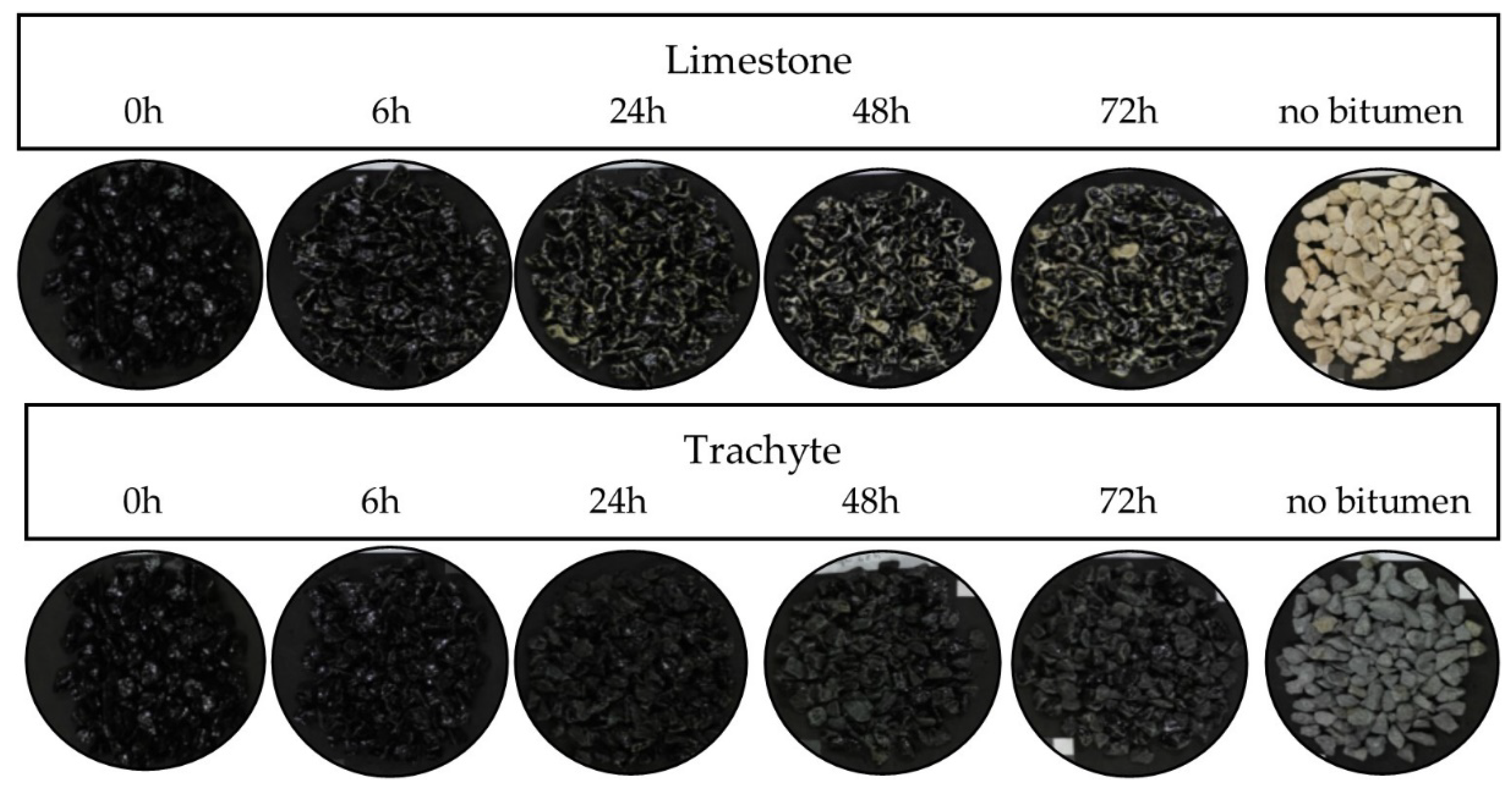
The adhesion tests were carried out at four different time steps: 6, 24, 48 and 72 h. For each step, three replicates were arranged for a total number of samples equal to 12. A bitumen-free sample and one totally coated sample completed the dataset. This combination was repeated for both limestone and trachytic aggregates for a total of 28 samples. Figure 3 shows photographs of the dataset of the materials obtained after the adhesion tests.

At the end of each time step, the specimens obtained were analyzed via operators’ visual inspection to estimate the percentage of bitumen coverage. To extend the statistical dataset, 16 operators were employed instead of the two required by the UNI EN 12697-11 [7] standard.

Figure 4 shows the large differences between the evaluations for each time step in terms of discrepancies between the minimum and maximum bitumen coverage values observed by the operators if compared to the averaged values. Standard deviations highlight discrepancies for trachytic samples, but, for both kinds of aggregates, a higher precision was obtained for the initial time steps.

The maximum and minimum values found within the evaluation forms show high heterogeneity. This fact was accentuated when the standard deviations were calculated for each sample and time step. Figure 4 shows the increase in these values from the evaluations carried out for trachyte (from 10.2 to 30.5) and limestone (from 6.7 to 11.6). On average, the standard deviations calculated for limestone and trachytic aggregates are 9.7 and 24.7, respectively, while the overall average considering both kinds of aggregates is 17.2. Lower standard deviations are related to the limestone samples while higher ones are related to trachyte ones. Because of the lower brightness difference between bitumen and trachytic aggregates, operators showed a greater difficulty in carrying out the quantification of bitumen coverage over aggregates.

To further highlight the high variability of such evaluations, the comparison of mean, median, and mode calculated for each sample shows how these values tend to coincide for the limestone samples while they tend to differ for the trachyte samples. In fact, the average standard deviations for trachyte and limestone samples are, respectively, 9.9 and 2.7.

3.2. Digital Imaging Processing

Digital pictures were acquired for each sample at every time step. An AOI, consisting of 743 rows × 761 columns (565,423 pixels), was fixed in the middle of each picture (dimensions 4928 × 3264 pixels) matching with the GIFOV of the spectrometers. All images were classified by applying the parallelepiped and the ISODATA algorithms. The classification of these images allowed obtaining an image with four classes: aggregates not coated by bitumen (exposed aggregates), aggregates coated by bitumen (not exposed aggregates), shadows, and reflections. The classification allowed quantifying the number of pixels corresponding to the four classes, which can be expressed as a percentage of the known area of 565,423 pixels. From each image classification, only the number of “exposed aggregates” was considered because of the major influence on the “not exposed aggregates” class of reflections and shadows. Separability analysis was performed to evaluate if such classes are easily separable. For each mixture, Jeffries–Matusita (JM) and transformed divergence (TD) values were calculated for “aggregates” and “bitumen” classes as ROIs. Limestone and trachyte aggregates showed respectively 1.97 and 1.21 for JM and 1.98 and 1.31 for TD separability measurements. As presented in [42], these measures can show values between 2 (completely separable) and 0 (no separability). Separability results corroborate a higher separability of limestone compared to trachytic aggregates.

The influence of shadows is minimized by a homogeneous illumination. Nevertheless, this influence must be considered as a limit of this kind of bi-dimensional analysis that does not allow considering the aggregate exposure of each aggregate in three dimensions.

Considering the above evidence, the values obtained from these classifications were expressed in terms of the exposed aggregate index. Finally, the BIT index was computed to achieve the percentage of bitumen coverage.

Figure 5 shows the results obtained with the two algorithms. The average values of the two methods tend to remain similar at the initial test stages but highly differ with the increase of the temporal steps. This was caused by the increase of the sample heterogeneity and the brightness variability of limestone or trachytic samples. These modifications affected the classification results obtained with the two algorithms, which used different criteria to define each class. Generally, values obtained for limestone aggregates show similar results for samples from each of the first three-time steps. Conversely, trachyte samples show a great variability. This evidence is better appreciated with the calculation of standard deviations and confusion matrices (overall accuracy and k-coefficient) of each image classification.

The parallelepiped method shows lower standard deviation values (1.38 for trachyte and 0.68 for limestone) than those obtained using the ISODATA method (16.80 for trachyte and 3.91 for limestone). For limestone mixtures, confusion matrices show the average overall accuracy (sum of the number of correctly classified values divided by the total number of values) and k-coefficient (measurement of the agreement between truth values and classification) for all rolling-bottle steps of 94.7% (k = 0.91) and 99.1% (k = 0.98) for ISODATA and parallelepiped, respectively. For trachytic mixtures, confusion matrices show average overall accuracy and k-coefficient of 79.7% (k = 0.72) and 98.3% (k = 0.97), respectively. The parallelepiped algorithm seems the most suitable technique to assess the BIT value for trachytic aggregates, while both techniques show remarkable results for both kinds of aggregates. Generally, higher overall accuracies are obtained for both aggregates with the parallelepiped algorithm.

3.3. Spectroscopy

The two VIS–NIR spectrometers were used to acquire spectral images of trachyte and limestone mixtures at 6, 24, 48 and 72 h. Once the dataset was developed, the hyperspectral cube was computed to manage and classify images. The number of images acquired by each camera was different because the frame rate of the two cameras was set to two different values, therefore more images were acquired by the sensor camera (frame rate equal to 50 fps) than by the Falcon camera (frame rate equal to 25 fps). By positioning the VIS spectrometer scan line perpendicular to the advancement direction of each sample, an image was obtained where each row (or column for NIR camera) represents the section of the scanned surface at a given wavelength. Through the initial step of the geometric calibration, a wavelength λ could be associated with each column of the image. The hyperspectral cube was processed using the ENVI^® (Environment for Visualizing Images, L3Harris Geospatial, Boulder, CO, USA) software program for visualization, analysis, and classification of digital images.

Radiometric calibration was performed to remove the dependence of the spectra on the measuring instruments. In fact, the acquisition system did not record the reflectance of the material but the radiance value, i.e., the part of the radiation reflected by the material that reaches the sensor and has sufficient energy to be recorded. Absolute reflectance can only be calculated if the radiation incident on the material is known. Since halogen lamps were used as the light source, it was not possible to calculate the incident radiation at each point of the scene. Thus, the relative reflectance was calculated, obtained by comparing the radiance of the materials with the reference spectrum of a suitably chosen material. A Halon tile of 10 cm side was used as a reference object, which was analyzed under the same lighting conditions and with the same experimental setup. The FF method was used for radiometric image calibration. This method considers the background noise associated with the sensor measurements and takes it into account by introducing the dark current, i.e., the radiance recorded through closed-objective measurements. The relation for the calculation of the reflectance ρ_λ is:

$${\mathsf{\rho }}_{\lambda }=\frac{R_{\lambda }-D_{\lambda }}{W_{\lambda }-D_{\lambda }}$$

(3)

where R_λ is the radiance of the material at the wavelength λ, D_λ is the value of the dark current, and W_λ is the radiance of the reference white (Halon tile).

At this stage, the cube presents spectral information along the x and y axes, which allows the identification of every single pixel of the image, and the spectral curve can be used to characterize and recognize the different materials. Spectral signatures of the various materials were extracted from the images by defining ROIs in the NIR and VIS images. The average spectral signature of a sample was then obtained by averaging the curves of all the pixels included within the sample area.

As done for digital pictures, separability analysis from aggregate to bitumen was performed for each mixture by JM and TD calculations. Trachyte and limestone aggregates showed for both spectrometers averaged values of 1.94and 2.00 for JM and 1.99 and 2.00 for TD, respectively. These data allowed supposing the suitability of both spectrometers, although the coarse pixel resolution of NIR spectrometer could represent a limitation for spatial accuracies.

Similar to the analyses carried out by DIP, the hyperspectral images were classified by the ISODATA and parallelepiped algorithms. These classifications were first used to calculate the EAI index and compute the BIT index for the bitumen coating over aggregates. Figure 6 shows trachyte and limestone samples after the rolling-bottle tests, while Figure 7 indicates BIT values at the different temporal steps for the two classifiers.

For trachytic mixtures, both techniques present remarkable accuracies for the VIS spectrometer, while the worst results were obtained with the NIR spectrometer. The results show no evident decrease of bitumen coverage at 48 and 72 h (about 77–71%), while the VIS spectrometer provides similar results (63% and 48%), and a decreasing trend can be observed. In addition, the accuracies reflect this discrepancy, showing lower values for the NIR ranges. This tendency is also evident for limestone aggregates, while a decreasing trend is more visible. In addition, in this case, accuracy values are higher for the VIS spectrometer. Generally, a good consistency of classification results was observed for ISODATA using the VIS spectrometer because of its higher spatial resolution.

The accuracy values were calculated through the application of the confusion matrix, which makes it possible, using reference ROIs for validation, to obtain the overall accuracy and kappa coefficient values, as done for digital images. For trachytic aggregates and VIS spectrometer data, the classification by ISODATA provides accuracy values of 94.3% and a kappa value of 0.88, while, in the NIR range, the accuracy is equal to 77.5% and the kappa is 0.50. For limestone aggregates and VIS spectrometer data, the classification by ISODATA provides accuracy values of 97.4% and a kappa value of 0.93, while, in the NIR range, the accuracy is equal to 91.4% and the kappa is 0.81. Therefore, accuracy tends to decrease from the VIS data to the NIR data. Furthermore, in the VIS range, the average standard deviation is 2.47 for trachyte and 1.15 for limestone, while, in the NIR region, it is 4.09 for trachyte and 3.03 for limestone. Therefore, for ISODATA, NIR-classified data generally seem to be less reliable than those obtained by classification in the VIS region.

The parallelepiped algorithm provides accuracy values of 87.4% and kappa equal to 0.74 in the VIS (standard deviation: 4.19), while these values are 70.8% and 0.35 in the NIR region for trachytic mixtures (standard deviation: 6.87). For limestone mixtures, the accuracy in the VIS region is 95.7% and the kappa is 0.90 (standard deviation: 3.47) while these values are 87.3% and 0.7 in the NIR range (standard deviation: 7.65). Generally, accuracies are higher for the VIS spectrometer (and standard deviations are higher in the NIR region). The accuracies obtained by ISODATA are generally higher than those obtained through the application of the parallelepiped method.

4. Discussion

The European Standard EN 12697-11 [7] focuses on different procedures for the determination of the affinity between aggregate and bitumen and its influence on the susceptibility of the combination to stripping. The bitumen coverage percentage over aggregates is evaluated by calculating the BIT index. In this study, the values calculated by DIP and VIS–NIR spectrometers were compared at each temporal step of the rolling-bottle test.

Therefore, the whole imaging classification dataset was compared for a better comprehension of the most suitable technique for bitumen coverage quantification. The dataset is composed of six different analyses, consisting of the application of ISODATA and parallelepiped algorithms to digital imagery and VIS/NIR hyperspectral cubes.

Figure 8 shows a decreasing trend of bitumen removal during the rolling-bottle test for each mentioned technique. Similar BIT values were observed at 6 and 24 h test steps, while, for longer temporal tests (48 and 72 h), a higher heterogeneity is prevalent. For each kind of classification technique, a lower reliability of measurements for longer tests was observed. Figure 9 highlights this trend by showing the standard deviation of the classification of both aggregate mixtures: at 6 and 24 h, standard deviations show lower values (1.50) than those obtained at 48 and 72 h (2.66). More specifically, for all the imaging algorithms, the variation of the average standard deviations of trachytic aggregates shows higher values (1.78 at 6/24 h and 3.34 at 48/72 h) when compared with those of limestone aggregates (1.22 at 6/24 h and 1.97 at 48/72 h).

The pie chart presented in Figure 10 summarizes the results of the different techniques, reporting the standard deviations (external ring) and the overall accuracies (internal ring) of each combination of processing technique, sensor, and aggregate type. Better results to retrieve the bitumen percentage coverage are differentiated for limestone and trachytic aggregates.

For limestone aggregates, higher results are reached with the use of VIS-spectrometer (97.4%) and digital pictures (99.1%), respectively, using ISODATA and parallelepiped techniques. For trachytic aggregates, overall accuracies are generally lower but, similar to limestone aggregates, better accuracies are reached using VIS spectrometer (94.3%) and digital pictures (98.3%), respectively, using ISODATA and parallelepiped techniques.

For both kinds of aggregates, the parallelepiped technique applied to digital pictures provides better results. These results are also expressed by the average standard deviations, which show values of 0.68 and 1.38, respectively, for limestone and trachyte.

In general, limestone mixtures show a lower standard deviation for the tested techniques, confirming the repeatability of the procedures. These results highlight the significance of spatial resolution rather than spectral resolution of the spectrometers used and the need of an initial start-up step defined by the user (supervised technique).

Figure 11 schematically represents the accuracies of each temporal test step obtained through the ISODATA and parallelepiped algorithms applied to both digital and hyperspectral images. Generally, higher accuracies are reached for limestone aggregates, but good results are also obtained for trachytic aggregates by using the VIS spectrometer (ISODATA) and digital picture (parallelepiped).

Considering the high subjectivity of each operator to determine the bitumen coverage percentage over aggregates and considering the high variability of the schematic reference scheme provided by the UNI EN 12697-11 [7] standard, the use of alternative and rapid methods seems to be crucial. In particular, the reference schemes refer to a detail of 5% among the evaluation classes for high-level covered samples and of the order of 10–20% for those with low-level cover.

Instead of the higher spectral resolution of the VIS spectrometer, the spatial resolution seems to be more efficient for this kind of analysis. Better pixel resolution of the VIS spectrometer should provide higher accuracies and might be more efficient for the bitumen coverage evaluation. At the same time, considering the minor costs of the photographic system compared to the spectrometers, the technique could be more cost-effective and therefore considered available in the UNI EN 12697-11 [7] as a smart standardized methodology. The elaboration of digital imaging can therefore represent an effective added value for a more rigorous determination of the affinity between aggregate and bitumen and its influence on the susceptibility of the combination to stripping. In addition, this kind of analysis allows simplifying the laboratory data processing operations and reduces subjective operator errors.

Further analyses will be focused on the use of different equipment and different aggregate and bitumen mixtures, with and without additives.

5. Conclusions

The determination of the affinity between aggregate and bitumen (UNI EN 12697-11 [7]) is evaluated in this paper by applying two different image algorithms. The ISODATA and Parallelepiped algorithms are applied to digital pictures and hyperspectral VIS–NIR images acquired by an optimized multi-sensor optical platform. Based on the application of these techniques, some main conclusion and remarks can be made:

• The application of image analysis can be a fast and effective way to quantify the loss of bitumen caused by the different test timings deriving from the rolling-bottle test.
• Better accuracies and reliability of measurements are shown when the VIS-spectrometer and digital pictures are used with the unsupervised and supervised algorithms, respectively.
• Instead, for the higher spectral resolution of spectrometers, higher spatial resolutions of digital pictures allow obtaining more reliable measurements.

Nevertheless, some features must be highlighted to overpass few critical steps of the adopted procedure:

• Optimize the sample preparation in order to minimize shadows effects.
• Build a more useful acquisition system in order to create a systematic and more rapid processing chain to calculate the bitumen affinity.
• Optimize the elaboration flow by the use of calculation codes able to pre-treat, calibrate, and then classify the image dataset.

In accordance with other studies, the results of this investigation reveal the possibility to implement a standardized analysis methodology using both digital and hyperspectral imagery to resolve inaccuracies of visual interpretation during operator’s analysis. In fact, the application of this method therefore represents an effective opportunity to provide another technique which allows to make rapid quantification despite a visual interpretation which, currently, is the most used standard technique in laboratories due to its simplicity and low costs. As shown, the application of a hyperspectral device does not provide better results than digital imaging processing, which seems to be the most suitable and usable system in common laboratory framework. Future tests will be addressed by considering the presented critical steps and using a different camera to be compared with digital pictures. In addition, different binders will be tested such as modified binders to evaluate their influence to its affinity to the aggregates.

References

1. Claine, P.J. Chemical composition of asphalt as related to asphalt durability: State of the Art. Transp. Res. Rec. 1984, 999, 13–30. [Google Scholar]
2. Lamperti, R.; Lantieri, C.; Sangiorgi, C.; Bitelli, G.; Simone, A. Semi-automatic evaluation of the degree of bitumen coverage on bitumen-coated aggregates. In 8th RILEM International Symposium on Testing and Characterization of Sustainable and Innovative Bituminous Materials; Springer: Basel, Switzerland, 2016; pp. 15–24. [Google Scholar]
3. Herold, M. Spectral characteristics of asphalt road surfaces. In Remote Sensing of Impervious Surfaces; CRC Press: Boca Raton, FL, USA, 2007; pp. 237–247. [Google Scholar]
4. Shafabakhsh, G.H.; Ani, O.J. Experimental investigation of effect of Nano TiO2/SiO2 modified bitumen on the rutting and fatigue performance of asphalt mixtures containing steel slag aggregates. Constr. Build. Mater. 2015, 98, 692–702. [Google Scholar] [CrossRef]
5. Ameri, M.; Kouchaki, S.; Roshani, H. Laboratory evaluation of the effect of nano-organosilane anti-stripping additive on the moisture susceptibility of HMA mixtures under freeze–thaw cycles. Constr. Build. Mater. 2013, 48, 1009–1016. [Google Scholar] [CrossRef]
6. Costa, M.; Simone, A.; Vignali, V.; Lantieri, C.; Bucchi, A.; Dondi, G. Looking behavior for vertical road signs. Transp. Res. Rec. Part F 2014, 23, 147–155. [Google Scholar] [CrossRef]
7. European Standartd. EN 12697-11: Bituminous Mixtures—Test Methods for Hot Mix Asphalt—Part 11: Determination of the Affinity between Aggregate and Bitumen; European Standartd: Brusseles, Belgium, 2012. [Google Scholar]
8. Andreou, C.; Karathanassi, V.; Kolokoussis, P. Investigation of hyperspectral remote sensing for mapping asphalt road conditions. Int. J. Remote Sens. 2011, 32, 6315–6333. [Google Scholar] [CrossRef]
9. Villa, P.; Boschetti, M.; Bianchini, F.; Cella, F. A hybrid approach for remote sensing multi-temporal mapping of urban areas in milan province, Italy. Eur. J. Remote Sens. 2012, 45, 333–347. [Google Scholar] [CrossRef]
10. Herold, M.; Roberts, D. Spectral characteristics of asphalt road aging and deterioration: Implications for remote-sensing applications. Appl. Opt. 2005, 44, 4327–4334. [Google Scholar] [CrossRef] [PubMed]
11. Noronha, V.; Herold, M.; Gardner, M.; Roberts, D.A. Spectrometry and Hyperspectral Remote Sensing for Road Centerline Extraction and Evaluation of Pavement Condition. In Proceedings of the Pecora Conference, Denver, CO, USA, 13 November 2002. [Google Scholar]
12. Mei, A.; Fiore, N.; Salvatori, R.; D’Andrea, A.; Fontana, M. Spectroradiometric laboratory measures on asphalt concrete: Preliminary results. Procedia Soc. Behav. Sci. 2012, 53, 514–523. [Google Scholar] [CrossRef] [Green Version]
13. Mei, A.; Salvatori, R.; Fiore, N.; Allegrini, A.; D’Andrea, A. Integration of field and laboratory spectral data with multi-resolution remote sensed imagery for asphalt surface differentiation. Remote Sens. 2014, 6, 2765–2781. [Google Scholar] [CrossRef] [Green Version]
14. Shvetsov, M. Concerning some additional aids in studying sedimentary formations. Bull. Mosc. Soc. Natural. 1954, 29, 61–66. [Google Scholar]
15. Bessa, I.S.; Branco, V.T.F.C.; Soares, J.B. Evaluation of different digital image processing software for aggregates and hot mix asphalt characterizations. Constr. Build. Mater. 2012, 37, 370–378. [Google Scholar] [CrossRef]
16. Bruno, L.; Parla, G.; Celauro, C. Image analysis for detecting aggregate gradation in asphalt mixture from planar images. Constr. Build. Mater. 2012, 28, 21–30. [Google Scholar] [CrossRef]
17. Marinoni, N.; Pavese, A.; Foi, M.; Trombino, L. Characterization of mortar morphology in thin sections by digital image processing. Cem. Concr. Res. 2005, 35, 1613–1619. [Google Scholar] [CrossRef]
18. Elunai, R.; Chandran, V.; Gallagher, E. Asphalt concrete surfaces macrotexture determination from still images. IEEE T. Intell. Transp. 2011, 12, 857–869. [Google Scholar] [CrossRef] [Green Version]
19. Mei, A.; Manzo, C.; Bassani, C.; Salvatori, R.; Allegrini, A. Bitumen removal determination on asphalt pavement using digital imaging processing and spectral analysis. Open J. Appl. Sci. 2014, 4, 366–374. [Google Scholar] [CrossRef] [Green Version]
20. Manzo, C.; Mei, A.; Salvatori, R.; Bassani, C.; Allegrini, A. Spectral modelling used to identify the aggregates index of asphalted surfaces and sensitivity analysis. Constr. Build. Mater. 2014, 61, 147–155. [Google Scholar] [CrossRef]
21. TRejbal, J.; Prošek, Z.; Valentová, T. Assessment of adhesion between mineral aggregate and bituminous binder using digital image analysis. Acta Polytech. CTU Proc. 2018, 15, 126–130. [Google Scholar] [CrossRef]
22. TRejbal, J.; Valentová, T.; Horovà, T. Assessment of adhesion between bituminous binder and mineral aggregate using digital image analysis. Acta Polytech. CTU Proc. 2019, 21, 38–41. [Google Scholar] [CrossRef]
23. Grönniger, J.; Wistuba, M.P.; Renken, P. Adhesion in bitumen-aggregate-systems. new technique for automated interpretation of rolling bottle tests. Road Mater. Pavement 2010, 11, 881–898. [Google Scholar] [CrossRef]
24. Källén, H.; Heyden, A.; Åström, K.; Lindh, P. Measuring and evaluating bitumen coverage of stones using two different digital image analysis methods. Measurement 2016, 84, 56–67. [Google Scholar] [CrossRef]
25. Lantieri, C.; Lamperti, R.; Simone, A.; Vignali, V.; Sangiorgi, C.; Dondi, G.; Magnani, M. Use of image analysis for the evaluation of rolling bottle tests results. Inter. J. Pavement Res. Technol. 2017, 10, 45–53. [Google Scholar] [CrossRef]
26. Riekstins, A.; Haritonovs, V.; Balodis, A. Evaluation of adhesion between bitumen and aggregate with the digital image processing method. In Proceedings of the 4th International Conference on Innovative Materials, Structures and Technologies, Riga, Latvia, 25–27 September 2019; p. 660. [Google Scholar]
27. Moghaddam, A.S. Estimation of Stripping by Static Immersion Test Using Image Processing and Machine Learning. Master’s Thesis, Lakehead University, Thunder Bay, ON, Canada, 2019. [Google Scholar]
28. Margaritis, A.; Tofani, G.; Jacobs, G.; Blom, J.; Tavernier, S.; Vuye, C.; Van den bergh, W. On the applicability of ATR-FTIR microscopy to evaluate the blending between neat bitumen and bituminous coating of reclaimed asphalt. Coating 2019, 9, 240. [Google Scholar] [CrossRef] [Green Version]
29. Caputo, P.; Miriello, D.; Bloise, A.; Baldino, N.; Mileti, O.; Ranieri, G.A. A comparison and correlation between bitumen adhesion evaluation test methods, boiling and contact angle tests. Int. J. Adhes. Adhes. 2020, 102, 102680. [Google Scholar] [CrossRef]
30. Moroni, M.; Dacquino, C.; Cenedese, A. Mosaicing of hyperspectral images: The application of a spectrograph imaging device. Sensors 2012, 12, 10228–10247. [Google Scholar] [CrossRef]
31. Moroni, M.; Lupo, E.; Cenedese, A. Hyperspectral proximal sensing of salix alba trees in the sacco river valley (Latium, Italy). Sensors 2013, 13, 14633–14649. [Google Scholar] [CrossRef] [Green Version]
32. Balsi, M.; Moroni, M.; Chiarabini, V.; Tanda, G. (2021). High-resolution aerial detection of marine plastic litter by hyperspectral sensing.remote sensing. Remote Sens. 2021, 13, 1557. [Google Scholar] [CrossRef]
33. Moroni, M.; Mei, A.; Leonardi, A.; Lupo, E.; Marca, F.L. PET and PVC separation with hyperspectral imagery. Sensors 2015, 15, 2205–2227. [Google Scholar] [CrossRef]
34. Moroni, M.; Mei, A. Characterization and separation of traditional and bio-plastics by hyperspectral devices. Appl. Sci. 2020, 10, 2800. [Google Scholar] [CrossRef] [Green Version]
35. European Standartd. EN 12697-2: Bituminous Mixtures—Test Methods–Part 2: Determination of Particle Size Distribution; European Standartd: Brusseles, Belgium, 2015. [Google Scholar]
36. European Standartd. EN 12697-35. Bituminous Mixtures—Test Methods—Part 35: Laboratory Mixing; European Standartd: Brusseles, Belgium, 2016. [Google Scholar]
37. Tou, J.T.; Gonzalez, R.C. Pattern Recognition Principles; Addison-Wesley Publishing Company: Boston, MA, USA, 1974. [Google Scholar]
38. Irvin, B.J.; Ventura, S.J.; Slater, B.K. Fuzzy and isodata classification of landform elements from digital terrain data in Pleasant Valley, Wisconsin. Geoderma 1977, 77, 137–154. [Google Scholar] [CrossRef]
39. Mausel, W.; Kramber, W.J.; Lee, J.K. Optimum band selection for supervised classification of multispectral data. Photogramm. Eng. Remote Sens. 1990, 56, 55–60. [Google Scholar]
40. Richards, J.A.; Jia, X. An Introduction. In Remote Sensing Digital Image Analysis; Springer: Berlin, Germany, 2006; pp. 267–294. [Google Scholar]
41. Albert, T.H. Evaluation of remote sensing techniques for ice-area classification applied to the tropical quelccaya ice cap, Peru. Polar Geogr. 2002, 26, 210–226. [Google Scholar] [CrossRef]
42. Jensen, J.R. Introductory Digital Image Processing: A Remote Sensing Perspective; Prentice Hall: Hoboken, NJ, USA, 1996. [Google Scholar]
Figure 1. (a) The three bottles containing the mixtures during the rolling-test; and (b) typical results of the rolling-bottle method.
Coatings 11 00648 g001
Figure 2. (a) Picture of the three-sensor platform used for this study, composed of conveyor belt, two light sources, digital camera, and VIS and NIR spectrometers; and (b) scheme of the hyperspectral device configuration.
Coatings 11 00648 g002
Figure 3. Samples obtained after each rolling-bottle time step for limestone and trachytic aggregates.
Coatings 11 00648 g003
Figure 4. Bitumen coverage trend obtained via visual inspection. The plot shows the minimum, maximum, averaged values, and trend of standard deviation variation during the rolling time.
Coatings 11 00648 g004
Figure 5. BIT computation by the Parallelepiped and the ISODATA algorithms.
Coatings 11 00648 g005
Figure 6. Limestone and trachytic samples acquired with the VIS spectrometer during the rolling-bottle test.
Coatings 11 00648 g006
Figure 7. BIT index and accuracies calculated by ISODATA and parallelepiped classifications for limestone and trachytic aggregate mixtures in both VIS and NIR ranges.
Coatings 11 00648 g007
Figure 8. BIT values obtain by different techniques for each HMA and test step.
Coatings 11 00648 g008
Figure 9. Standard deviation trend calculated for each mixture and technique at every rolling-bottle time test.
Coatings 11 00648 g009
Figure 10. Pie charts of overall accuracies and standard deviations computed for each imaging technique using: (a) limestone; and (b) trachyte aggregates.
Coatings 11 00648 g010
Figure 11. Averaged overall accuracy for each mixture and technique during the rolling-bottle test.
Coatings 11 00648 g011