Abstract
Compacted graphite iron (CGI), having a specific graphite form with a large matrix contact surface, is a unique casting material. This type of cast iron tends to favor direct ferritization and is characterized by a complex of very interesting properties. Intelligent computing tools such as artificial neural networks (ANNs) are used as predictive modeling tools, allowing their users to forecast the microstructure of the tested cast iron at the level of computer simulation. This paper presents the process of the development of a metamodel for the selection of a neural network appropriate for a specific chemical composition. Predefined models for the specific composition have better precision, and the initial selection provides the user with automation of reasoning and prediction. Automation of the prediction is based on the rules obtained from the decision tree, which classifies the type of microstructure. In turn, the type of microstructure was obtained by clustering objects of different chemical composition. The authors propose modeling the prediction of the volume fraction of phases in the CGI microstructure in a three-step procedure. In the first phase, k-means, unsupervised segmentation techniques were used to determine the metamodel (DT), which in the second phase enables the selection of the appropriate ANN submodel (third phase).
1. Introduction
Compacted graphite iron (CGI) has been known since 1948, but its use only took place in the late 1960s, when serial production of automotive parts made of ferritic CGI began in Austria []. Its production process requires maintaining a strict technological regime due to the narrow concentration range of elements ensuring the compacted (vermicular) shape of graphite. Owing to its unique properties combining good tensile strength with high thermal shock resistance, it is mostly used in the automotive industry. An example of a CGI microstructure is shown in Figure 1a,b.
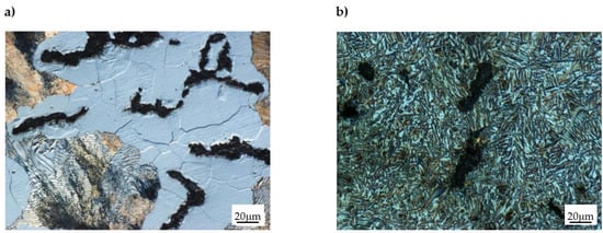
Figure 1.
Different microstructures of CGI: ferritic-pearlitic (a) [], ausferritic (b) [].
The matrix of unalloyed CGI usually consists of ferrite and pearlite (Figure 1a). Due to the large contact surface of graphite with the metal matrix, this cast iron is characterized by a greater tendency to form ferrite compared to nodular or grey cast iron. As defined in EN-16079 standard, the typical CGI microstructure provides a minimum tensile strength of 300 to 500 MPa. To obtain pearlite, copper, nickel, or tin are used. Due to the unique properties of CGI, the technology is still being developed, which is reflected in many publications [,,,,,,,,,]. There is a lot of information on the effect of alloy additions on the microstructure and the properties of CGI, e.g., [,,]. As in nodular cast iron, in CGI it is also possible to obtain an ausferrite as a result of heat treatment [,,,]. Such cast iron is sometimes referred to as austempered vermicular iron (AVI) or austempered vermicular cast iron (AVCI). Ausferrite is a mixture of bainitic ferrite and high carbon austenite. To obtain the ausferrite in cast iron, the austempering process is required. Its course is shown in Figure 2.
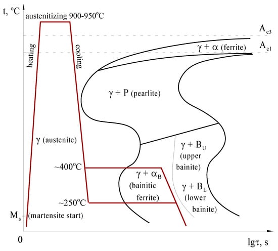
Figure 2.
The course of heat treatment in ADI or AVI.
The essence of such heat treatment (called austempering) is heating to the austenitization temperature (approx. 900–950 °C) and holding at that temperature to obtain an austenite in the cast iron matrix. The next step is quenching in a salt bath at 400–250 °C. The isothermal holding time must be short enough to prevent the precipitation of carbides, which decrease the elongation. Carbide precipitation would result in the formation of bainite (upper and/or lower).
There is also an alternative way to obtain the ausferritic matrix, i.e., by modifying the chemical composition of cast iron, using molybdenum together with copper or nickel [,,]. The microstructure of ausferritic CGI is shown in Figure 1b. The key element is molybdenum, which significantly increases the stability of austenite in the pearlitic area but does not significantly change it in the bainitic area, as schematically shown in Figure 3. Experimental data on the effect of molybdenum on the stability of austenite on continuous cooling transformation (CCT) can be found in [].
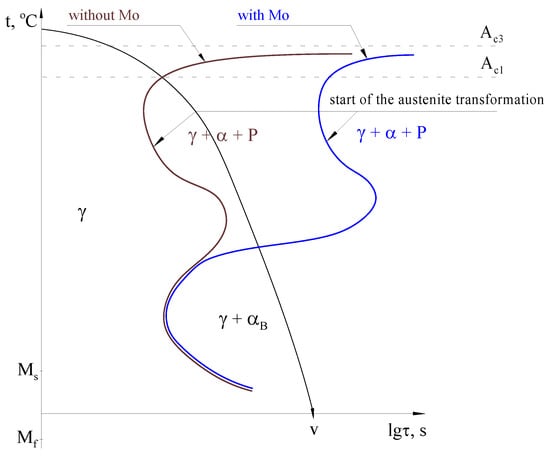
Figure 3.
The effect of molybdenum on the austenite stability α—ferrite, γ—austenite, P—pearlite, αB—bainitic ferrite [].
As shown in Figure 3, for the same cooling rate “v”, in cast iron without Mo, austenite will transform into ferrite and pearlite, while in cast iron with Mo, austenite will transform into bainitic ferrite. It allows the production of CGI without the use of heat treatment.
In the era of Industry 4.0, when all processes are successively automated and production is moving towards the model of cyber-physical systems, there is still room for human creativity. The needs and threats related to this aspect of the industrial revolution have been the subject of scientific publications for several years [,,]. Artificial intelligence allows us to improve people’s work and optimize processes, but it still often requires the human operator to make decisions. The role of humans is also essential in creating system concepts, in designing and planning production, or in designing new materials, and in these areas it remains unchallenged so far. Artificial intelligence can only solve clearly defined problems. Defining problems requires imagination and the ability to anticipate technological barriers to future concepts that only humans can boast of. The difference in artificial intelligence methods, such as data mining and machine learning, is also worth emphasizing. In many respects, data mining and machine learning are made up of the same group of algorithms. The main difference lies in the intended use of the results obtained by these methods. Machine learning leads to black box models to be processed by computer, to enable the machine to make decisions. Data mining is primarily aimed at discovering the knowledge that is contained in data structures, relationships, and patterns, but in the case of data mining, the beneficiary is the human being. Man should be given explanations; the result in numbers is not enough. The engineer expects a description of reality, a dependency model, and information on what basis a given solution has been obtained. This explains the popularity of methods called Explainable Artificial Intelligence, the purpose of which is to explain the rationale behind decisions made by artificial intelligence models. Individual algorithms used in intelligent data analysis have different levels of interpretability—the group of methods called decision trees [,,], which was very popular for many years, has been replaced by more precise techniques, i.e., artificial neural networks or support vector machines [], both offering greater precision at the expense of ease of interpretation. There is now a return to simpler (more transparent) methods for humans, but which are modified to increase efficiency. Unsupervised learning methods, i.e., cluster analysis, are also used to discover patterns between objects (materials, processes, etc.).
The problem analyzed by the authors of this paper concerns the prediction of the volumetric fraction of phases in the microstructure of compacted graphite iron. The problem is related to the earlier research conducted by the authors [,], but this time the focus is on a higher level of inference. The prediction of phases in a microstructure with division into individual constituents, particularly ausferrite, has already been partially resolved. However, a comprehensive model that would allow the experimenter to fit an appropriate model to the prediction of each of the constituents was still missing.
The use of ML methods in metal engineering is becoming more and more popular []. There are many works that deal with the use of supervised learning (ANN [], kNN [], and DTs [], and others such as XGBoost or ridge regression []) in predicting the properties of metals and works indicating the possibility of using unsupervised learning, especially k-means, in image segmentation [].
The use of machine learning methods to predict material properties is a very interesting topic. In [,], ML methods were used to link defects with mechanical properties. In many works, the use of ML tools was used to improve the level of control over the production process [].
However, the most similar studies to those presented in this article concern the prediction of the properties of metals. An example of such research is the use of neural networks to predict properties [,] or to predict the properties of new Fe2.5Ni2.5CrAl alloys [].
It is much more difficult to find examples of research using ML tools in the analysis of CGI properties. The latest publications on this material use either qualitative analysis [,,] or the traditional statistical approach to search for dependencies and build linear regression models [,].
The presented manuscript presents an innovative approach to the topic of microstructure-based property modeling. Supervised modeling techniques (ANN) adapted to the characteristics of different phases, and unsupervised techniques (k-means) for segmentation allowing for metamodel determination (DTs), which enables the selection of the correct submodel, were both used.
The solution proposed in this article consists of several elements, including both the white-box elements (classification trees), allowing the discovery of relationships and easy interpretation for an expert in the field of material design, and the black-box elements (neural networks), allowing for precise prediction of the contribution of individual microstructures. This approach combines the advantages of both techniques, allowing not only an easy interpretation of dependencies, but also precise prediction. An additional advantage is also the automation of the data analysis procedure (using k-means clustering) and microstructure prediction using data-driven models, which is expected to speed up and optimize the process of experimental design of products cast from various types of compacted graphite iron.
2. Experimental Methods and Data Acquisition
The cast iron for testing was melted in an electric induction furnace with a capacity of 30 kg (ELKON Company, Rybnik, Poland). For melting the cast iron, a crucible made of MINRO SIL 1001 refractory material by Allied Mineral Products was used. The charge was special pig iron with the chemical composition given in Table 1.

Table 1.
Chemical composition of special pig iron.
The content of Si was controlled with ferrosilicon FeSi75 and the content of Mn with ferro-manganese FeMn75; technically, pure Mo, Ni, Cu, Sn and Cr were used as alloying additives. After melting, the cast iron was overheated to a temperature of 1520–1530 °C and then poured into a sand mold. The pouring temperature was about 1460–1480 °C. Magnesium treatment was carried out by the Inmold process. This consists of placing the master alloy in the gating system inside a spherical reaction chamber having an 85 mm diameter. The shape and dimensions of the test casting are shown in Figure 4. The chemical composition of the master alloy is given in Table 2.
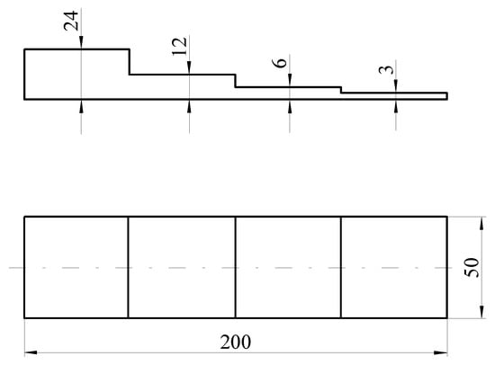
Figure 4.
Shape and dimensions of the test casting.

Table 2.
Chemical composition of the master alloy.
Cooling of the casting to ambient temperature took place in the mold. After knocking it out from the mold, the casting was cleaned and the gating system was cut off. The chemical composition of cast iron was determined on a SPECTROMAXx Arc Spark OES metal analyzer from SPECTRO Analytical Instruments GmbH. An example of the chemical composition of the tested cast iron along with the content of the matrix components is shown in Table 3.

Table 3.
An example of the chemical composition of the tested cast iron along with the content of the matrix components.
According to the matrix composition, the examined cast iron was divided into four groups (clusters) with the following designations:
- FP—ferritic-pearlitic (pearlitic-ferritic),
- M—martensitic,
- AN—austenitic,
- AF—ausferritic.
Carbides were also present in the tested cast iron. Their number depended on both the chemical composition and the wall thickness of the casting.
3. Modeling Methods
3.1. Decision Trees
The decision tree is a method that can serve the purpose of both classification and regression; this study is focused on classification trees. The decision tree is treated as a graph G = (V, E) consisting of a finite, non-empty set of nodes (vertices) V and a set of edges (leaves) E. The root and internal nodes test a given attribute (or a set of attributes), while leaves correspond to the possible test results []. To predict the value of the dependent variable for a given instance, the user has to navigate through a decision tree. Starting from the root, he should follow the edges according to the results of tests made on the attributes. After reaching the leaf, the information contained in this leaf will be responsible for the result of the predictions, e.g., in the traditional decision tree solving the classification problem, this result will be the class label []. The most popular method of creating decision trees involves an induction algorithm based on a greedy, top-down, recursive tree growth partitioning strategy called Top-Down Induction []. To accurately induce decision trees, efficient algorithms have been developed. These algorithms usually use greedy strategies to develop decision trees in a top-down fashion, making a number of locally optimal decisions regarding the selection of an attribute to split the training set and to make a split within that attribute. One of the oldest decision tree induction algorithms is Hunt’s Concept Learning System Framework, which is the basis of many current decision tree induction algorithms, such as ID3, C4.5, and CART [,,].
3.2. Clustering
In the described solution, both the CART algorithm and the k-means grouping methods were used. This algorithm is one of the oldest and most popular unsupervised learning methods, used as a basis for the development of other tools []. Clustering searches for natural structures and groups of similar objects in a set of unmarked data []. In terms of computation, the algorithm comes down to two-criteria optimization, in which the distance between cluster objects is minimized and the distance between clusters is maximized []. The process of grouping similar objects is iterative through successive adjustments of k-clusters (groups) of objects in such a way that the mean-square distances of all elements from the k-centers are as small as possible. In subsequent iterations, individual objects are moved to the clusters with the centers located at the shortest distance. For new clusters created in this way, new resources are determined and another iteration takes place until the result is satisfactory []. In the case under discussion, this method will be used for grouping the results of experimental studies based on the phase composition, also taking into account the most important alloying additives.
3.3. Artificial Neural Networks
As a formal tool for building predictive models, this solution uses, among others, artificial neural networks (ANNs) [,,]. This formal knowledge representation method is used to model multidimensional nonlinear phenomena, and the data currently obtained describes such a phenomenon. The indisputable advantage of ANNs is their ability to independently discover relationships between variables by repeatedly presenting the network with training cases []. In the process of training the network, model cases are presented to the network and then, in accordance with the assumed training strategy, the connections between network elements, otherwise known as weighting factors, are modified. In this study, artificial neural networks were used to build predictive models that would allow predicting the percentage of constituents in the microstructure of CGI iron depending on the chemical composition currently used.
4. Model Construction Procedure
The procedure of creating prediction models for the percentage composition of the CGI microstructure was developed in parallel with the influx of experimental data, which included subsequent chemical components and their proportional fractions. However, only models driven by the latest data set should be included in the analysis and comparison. Some attention is deserved for the fact that each record in the data set is a separate experimental melt, and its properties and chemical composition constitute a separate, unique, and unrepeatable result. Obtaining this type of data is a tedious and costly process, requiring careful examination of each object in the database and interrelationships between individual objects. The diagram in Figure 5 represents the idea of comparing three variants of the modeling procedure. The variant marked with number 1 is a classic approach; using a data set, we train neural networks to obtain, from the output, the percentage of each CGI phase, i.e., ferrite, pearlite, martensite, austenite, and ausferrite. This approach is a common way to start research and uses a comparative model.
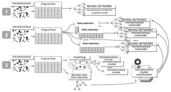
Figure 5.
Schemes of three variants of conducting research and relations between the models.
More focused research involves creating and training separate neural networks for each phase (constituent) of the microstructure. In variant 2, depending on the microstructure composition, the data set is split into separate partitions. For each partition, a network is trained, and it returns the prediction of the content of a given constituent depending on the alloy chemical composition. Therefore, several models are obtained, and their application depends on the chemical composition and the knowledge of the expert/analyst who will use a specific model for the purpose of prediction. However, this expert must know the rough effect of a given chemical composition. This means that to predict the microstructure, the expert must know at the stage of designing the chemical composition what phase can be expected at the output, as only then he will be able to choose a model that will precisely determine the quantitative content of this phase. Hence it follows that, although the procedure is quite precise, it places great demands on the expert and the assumptions may result in an error if the wrong model has been chosen.
To avoid such doubts, variant 3 was developed (Figure 5).
Variant 3 creates a metamodel that determines the selection of an appropriate submodel. This metamodel is designed to capture the knowledge about the basic relations prevailing in the data set, including relations between the microstructure composition and the type of alloying additives. The metamodel is therefore intended to replace the rough knowledge about the resulting composition of the microstructure and to run the correct submodel allowing for precise prediction. The metamodel used in this study was constructed using two machine learning techniques. Unsupervised learning (clustering) was used to obtain groups of materials with a similar microstructure and chemical composition, and then, for these groups (clusters), a classification tree was induced which, based on the chemical composition of the sample, was able to indicate the correct class of microstructure. In this way, the appropriate submodel of the ANN network was selected, allowing for further precise prediction of the quantitative percentage composition of the microstructure.
5. Results and Discussion
The collected experimental data included the chemical composition of the melts (C, Si, Mn, Cr, Sn, Cu, Ni, Mo), the thickness of the casting wall, and the percentage composition of the microstructure (ferrite, pearlite, carbides, martensite, ausferrite, austenite). The statistical analysis was performed to explore the relationship between the content of individual elements of the chemical composition and the content of microstructural constituents. The results of this analysis indicated that the content of individual microstructural constituents (where ferrite and pearlite were combined into one group designated FP, taking also into account martensite—M; austenite—AN; and ausferrite—AF) depends mainly on two elements added to the alloy chemical composition, i.e., nickel and molybdenum (Figure 6). The results of the analysis were used as a starting point for the selection of variables in the next step of the procedure, which was grouping.
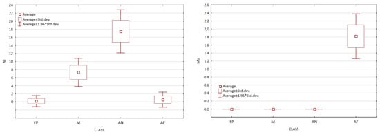
Figure 6.
Boxplot charts of the content of individual microstructural constituents depending on the addition of nickel and molybdenum.
5.1. Clustering
Grouping of objects was undertaken to create clusters used later for classification. The task of the clusters was to group together melts with a similar chemical composition and, most of all, with a similar composition of microstructure. Therefore, the indicated microstructural constituents were selected for the k-means analysis. As a result of the cluster analysis, five clusters of different size were obtained (Table 4, Figure 7). The error in the training sample was 0.132.

Table 4.
Means of clusters (k-means method). Number of clusters: 5. Total number of learning cases: 200.
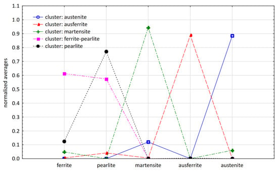
Figure 7.
The content of individual microstructural constituents in clusters (cluster numbers are replaced with verbal descriptions).
The clustering quality was assessed by comparing the resulting classification (assigning each record to a cluster) with the judgment of an expert who manually classified each case based on the data and using the following labels: ferritic-pearlitic—FP; martensitic—M; austenitic—AN; and ausferritic—AF. It was necessary to join clusters 4 and 5, i.e., the ferritic and ferritic-pearlitic clusters and, as a result of this operation, only four clusters were left. Compared with expert judgment, the clustering operation gave satisfactory results (Table 5).

Table 5.
Summary of the goodness of fit of the clustering results with expert judgment.
Out of 200 records, only one had a different assignment (non-compliance at the level of 0.5%) (Table 6).

Table 6.
Cardinality table for clustering (Cluster). Observation variable: Class.
5.2. Decision Trees and Rule Induction
The CART algorithm for induction of classification trees was implemented for the complete data set. The model was found to be in line with previous statistical analyses. The two most important alloying elements, i.e., molybdenum and nickel, have a decisive influence on the formation of different types of microstructure. Testing the content of each of them allows predicting what microstructure will arise as a result of making a melt with a given composition.
The tree presented in Figure 8 consists of four levels and four leaves. Molybdenum (Mo) was proven to be the attribute that best splits the set in the root. It is split into {‘FP’}—ferritic-pearlitic node and {‘AF’}—ausferritic leaf. As the best splitting attribute, the node using the {‘FP’} partition selected nickel, which has two nodes, i.e., the {‘FP’} leaf and the {‘M’} node denoting the martensitic cast iron. Based on the upper nickel content, the {‘M’} node undergoes the last splitting operation into the {‘M’} martensitic and {‘AN’} austenitic leaves. The test levels (values) are shown in Figure 8.
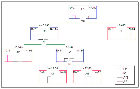
Figure 8.
The decision tree (CART) allowing its user to predict the type of microstructure formed as a result of a given chemical composition.
For a complete data set, the CART tree was found to be almost flawless. Only in one out of 200 records, a misclassification occurred (Figure 9). It was the same case that had been wrongly assigned to the cluster by the k-means method. This record was described by an expert as ausferritic. Its composition, however, indicated only 27% ausferrite, 36% pearlite, and 37% carbides, which would suggest that it was actually a ferritic-pearlitic cast iron. This, in turn, means that the classification made by the tree was consistent with that made by the expert, despite the fact that, in the training data, the label was assigned according to the algorithm response. In this way, it was proved through misclassification that the tree made an error-free assignment.
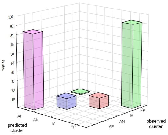
Figure 9.
The results of the CART tree classification. The single error is in case 137. The tree made the classification consistent with that made by an expert, and the error is only related to the clustering result.
Four rules were coded in the form of a tree, allowing for the selection of an appropriate microstructure, and thus launching an appropriate prediction model based on the artificial neural networks (ANNs).
5.3. Artificial Neural Networks
The process of building a neural network model consists of the following stages: defining explanatory and dependent variables; selecting the type and determining the structure of the neural network; training the neural network; and evaluating the network model. This section describes the steps of creating neural network models for the first two variants of the model construction procedure presented in Figure 10.
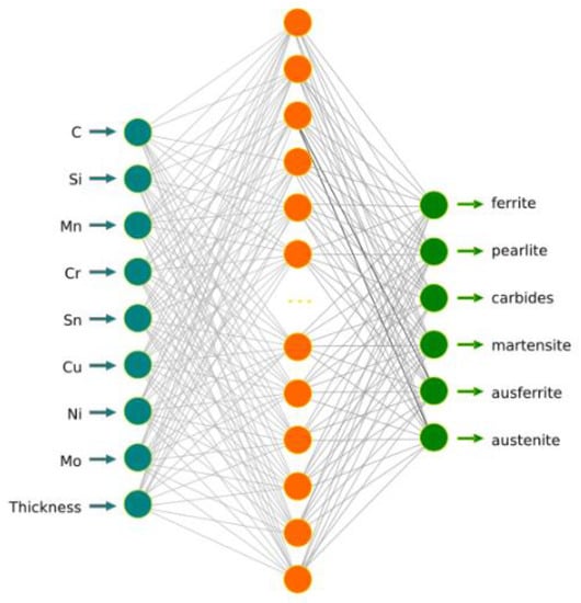
Figure 10.
Global ANN model—MLP 9-17-6.
In the first stage of the research, all the explanatory and dependent variables appearing in the experimental data set were used to build one global model of the neural network. Therefore, according to Table 3, the designed network should contain nine neurons in the input layer (these are eight neurons determining the content of individual elements of the chemical composition and one neuron determining the thickness of the casting wall) and six neurons in the output layer (each of them describes the content of a particular constituent in the microstructure of the tested CGI iron). The advanced analytics software package Statistica was used to define the detailed architecture of the network. Several hundred architectures were generated with different numbers of neurons in the hidden layer and different activation functions in the hidden layer and in the output layer. Out of all networks generated by the program, the MLP network with the MLP 9-17-6 architecture was selected. It was characterized by a high coefficient of determination and the lowest validation error. The structure of the developed network is shown in Figure 10.
In this network, the Broyden–Fletcher–Goldfarb–Shanno (BFGS) method [,] was used for training. The training process was completed in epoch 281. The coefficients of determination (R2) assumed the following values: training set—0.99; test set—0.94; validation set—0.94. The detailed parameters of the developed network are summarized in Table 7.

Table 7.
Detailed parameters of the developed network.
To perform a detailed analysis of the prediction values for individual dependent variables, where each of these variables describes the content of individual microstructural constituents, for each of the variables, the quality parameters, i.e., an absolute error and the coefficient of determination R2, were determined. Table 8 gives the basic quality parameters of the developed network. Figure 11 shows the scattering diagrams based on the observation results and the results generated from the developed MLP 9-17-6 network model for individual dependent variables, i.e., (a) ferrite, (b) pearlite, (c) carbides, (d) martensite, (e) ausferrite, (f) austenite.

Table 8.
Basic characteristics of the developed global ANN model—MLP 9-17-6.
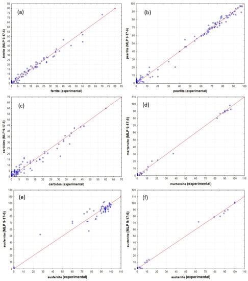
Figure 11.
Correlation charts based on the observation results and the results generated from the developed MLP 9-17-6 network model: (a) ferrite, (b) pearlite, (c) carbides, (d) martensite, (e) ausferrite, (f) austenite.
As follows from Table 8, the best model fit, i.e., the determination coefficient R2 of 0.995 and the smallest Mean Absolute Error (MAE) of 0.869, has the variable determining the percentage of austenite content. The worst model fit, i.e., the determination coefficient R2 of 0.841 and the largest Mean Absolute Error (MAE) of 2.81, has the variable determining carbide content in the microstructure.
To search for solutions with even better goodness of fit parameters, studies were carried out to create several separate neural networks, each for a different constituent of the microstructure. As part of these studies, six separate neural networks were designed (Figure 12). They all contained the same number and type of explanatory variables, while the dependent variable differed in each case, including ferrite, pearlite, carbides, martensite, ausferrite, and austenite.
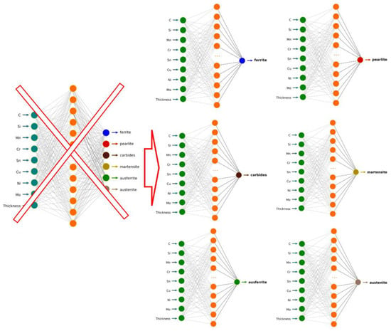
Figure 12.
Diagram of the structure of partial network models.
The basic characteristics of the developed networks and their quality parameters are compared in Table 9. The analysis of the results shows a general improvement in the quality of prediction models in relation to the global model, in particular a clear improvement for the carbide phase, which was the one least represented in the global model.

Table 9.
Basic characteristics of the developed networks and their quality parameters.
5.4. Discussion
The discussed issue concerns the prediction of the volume fraction of phases in the CGI microstructure. Previous studies [,] developed prediction models, in particular of ausferrite, but this time the focus was on a higher level of inference. Building separate models for individual phases has shown the possibility of increasing the accuracy of prediction and has already been partially resolved. However, there was still no comprehensive model that enabled the experimenter to choose an appropriate model to predict each component. In the present study, the authors propose the modeling of properties based on the microstructure in a three-step procedure. In the first phase, k-means, unsupervised segmentation techniques were used to determine the metamodel (DT), which in the second phase enables the selection of the appropriate ANN submodel (third phase). Such a solution allows the use of models that are relatively simple and easy to interpret, resulting in an efficient architecture that allows for a quick and precise assessment of the future phase composition in the CGI microstructure. The solution proposed in this article consists of several elements, including both components that allow for the discovery of dependencies and easy interpretation by an expert (DTs), supporting and facilitating the prediction of properties, and components that allow for precise prediction of the contribution of individual microstructures (ANN). This approach combines the advantages of both techniques, allowing not only easy interpretation of dependencies, but also precise prediction. An additional advantage is the automation of the data analysis procedure (using k-means clustering), which accelerates and optimizes the CGI design process.
Earlier works by the authors developed prediction models for individual phases []. The most difficult phase is to predict the content of ausferrite; hence, the accuracy of the models responsible for this component in the best models reached R2 = 0.87 (ANN); SVM R2 = 0.81; CART R2 = 0.83. The current architecture allowed the forecasting efficiency to be increased to R2 = 0.97.
6. Summary
The presented methodology of data-driven model selection for compacted graphite iron microstructure prediction was found to be very effective for the experimental data set. Its use improved the overall prediction of the microstructure composition, and at the same time allowed for an automatic model selection depending on the chemical composition. A side effect of the research was the detection of a special case in the training set, which in itself is an added value. This makes the authors believe that with the increasing size of the training database as a result of subsequent material experiments, it will also be possible to successfully apply the indicated approach to designing new, experimental chemical compositions, possibly including other alloying additives. At present, for these specific data, the metamodel makes accurate classifications. The single case that resulted in a wrong decision was only a confirmation of the rule; it allowed drawing interesting conclusions by pointing to differences that are difficult for the machine to identify, and for a human it was a special case and a valuable clue in further analyses. Once again it is easy to notice that although the role of artificial intelligence in developing Industry 4.0 is invaluable, human intelligence remains an indispensable element of our reality.
Author Contributions
Conceptualization, G.G., B.M. and K.R.; Data curation, G.G. and B.K.; Formal analysis, B.M. and K.R.; Funding acquisition, G.G. and K.R.; Investigation, G.G.; Methodology, G.G., B.K., B.M. and K.R.; Project administration, G.G.; Supervision, G.G.; Validation, B.M. and K.R.; Writing—original draft, G.G., B.M. and K.R.; Writing—review and editing, G.G., B.M. and K.R. All authors have read and agreed to the published version of the manuscript.
Funding
This study was carried out as part of the fundamental research financed by the Ministry of Science and Higher Education, grant No. 16.16.110.663 (B.M., K.R.).
Institutional Review Board Statement
Not applicable.
Informed Consent Statement
Not applicable.
Data Availability Statement
All data that support the findings of this study are included within the article.
Conflicts of Interest
The authors declare no conflict of interest. The funders had no role in the design of the study; in the collection, analyses, or interpretation of data; in the writing of the manuscript; or in the decision to publish the results.
References
- Nechtelberger, E.; Puhr, H.; Nesselrode, J.B.; Nakayasu, A. Stand der Entwicklung von Gusseisen mit Vermiculargraphit—Herstellung, Eigenshaften und Anwendung. Teil 1. Giesserei-Praxis 1982, 22, 359–372. [Google Scholar]
- Gumienny, G.; Kurowska, B.; Fabian, P. Compacted graphite iron with the addition of tin. Arch. Foundry Eng. 2020, 20, 15–20. [Google Scholar]
- Gumienny, G.; Kacprzyk, B. Compacted Graphite Iron with the Matrix Consisting of an Ausferrite and Carbides. Patent No. PL416959A1, 28 June 2019. [Google Scholar]
- Zhu, J.; Liu, Q.; Jiang, A.; Lian, X.; Fang, D.; Dong, H. Effects of Cu on the Morphology and Growth Mode of Graphite in Compacted Graphite Iron. Trans. Indian Inst. Met. 2021, 74, 1529–1536. [Google Scholar] [CrossRef]
- Shi, G.Q.; Yang, Z.; Li, J.P.; Sun, S.; Guo, M.; Tao, D.; Ma, Z.J. Investigation into the Evolution of Microstructure and Mechanical Properties of Compacted Graphite Iron under Elevated Temperature. J. Mater. Eng. Perform. 2021, 30, 8479–8489. [Google Scholar] [CrossRef]
- Pina, J.C.; Shafqat, S.; Kouznetsova, V.G.; Hoefnagels, J.P.M.; Geers, M.G.D. Microstructural study of the mechanical response of compacted graphite iron: An experimental and numerical approach. Mater. Sci. Eng. A 2016, 658, 439–449. [Google Scholar] [CrossRef]
- Kopyciński, D.; Guzik, E.; Nowak, A.; Ronduda, M.; Sokolnicki, M. Preparation vermicular graphite in thin and thick wall iron castings. Arch. Foundry Eng. 2012, 12, 41–44. [Google Scholar] [CrossRef]
- Guo, Y.; Stalbaum, T.; Mann, J.; Yeung, H.; Chandrasekar, S. Modulation-assisted high speed machining of compacted graphite iron (CGI). J. Manuf. Processes 2013, 15, 426–431. [Google Scholar] [CrossRef]
- Da Silva, L.R.R.; Souza, F.C.R.; Guesser, W.L.; Jackson, M.J.; Machado, A.R. Critical assessment of compacted graphite cast iron machinability in the milling process. J. Manuf. Processes 2020, 56, 63–74. [Google Scholar] [CrossRef]
- Palkanoglou, E.N.; Baxevanakis, K.P.; Silberschmidt, V.V. Interfacial debonding in compacted graphite iron: Effect of thermal loading. Procedia Struct. Integr. 2020, 28, 1286–1294. [Google Scholar] [CrossRef]
- Górny, M.; Kawalec, M. Role of Titanium in Thin Wall Vermicular Graphite Iron Castings Production. Arch. Foundry Eng. 2013, 13, 25–28. [Google Scholar] [CrossRef][Green Version]
- Lyu, Y. Abrasive wear of compacted graphite cast iron with added tin. Metallogr. Microstruct. Anal. 2019, 8, 67–71. [Google Scholar] [CrossRef]
- König, M.; Wessén, M. The influence of copper on microstructure and mechanical properties of compacted graphite iron. Int. J. Cast Met. Res. 2009, 22, 164–167. [Google Scholar] [CrossRef]
- Popov, P.I.; Sizov, I.G. Effect of alloying elements on the structure and properties of iron with vermicular graphite. Met. Sci. Heat Treat. 2006, 48, 272–275. [Google Scholar] [CrossRef]
- Ghasemi, R.; Hassan, I.; Ghorbani, A.; Dioszegi, A. Austempered compacted graphite iron—Influence of austempering temperature and time on microstructural and mechanical properties. Mater. Sci. Eng. A 2019, 767, 138434. [Google Scholar] [CrossRef]
- Pytel, A.; Gazda, A. Evaluation of selected properties in austempered vermicular cast iron (AVCI). Trans. Foundry Res. Inst. 2014, 54, 23–31. [Google Scholar]
- Ramadan, M.; Nofal, A.A.; Elmahalawi, I.; Abdel-Karim, R. Comparison of austempering transformation in spheroidal graphite and compacted graphite cast irons. Int. J. Cast Met. Res. 2006, 19, 151–155. [Google Scholar] [CrossRef]
- Ferry, M.; Xu, W. Microstructural and crystallographic features of ausferrite in as-cast gray iron. Mater. Charact. 2004, 53, 43–49. [Google Scholar] [CrossRef]
- Gumienny, G.; Klimek, L.; Kurowska, B. Effect of the Annealing Temperature on the Microstructure and Properties of Ausferritic Nodular Cast Iron. Arch. Foundry Eng. 2016, 16, 43–48. [Google Scholar] [CrossRef][Green Version]
- Xu, W.; Ferry, M.; Wang, Y. Influence of alloying elements on as-cast microstructure and strength of gray iron. Mater. Sci. Eng. A 2005, 390, 326–333. [Google Scholar] [CrossRef]
- Gumienny, G.; Giętka, T. Continuous Cooling Transformation (CCT) Diagrams of Carbidic Nodular Cast Iron. Arch. Metall. Mater. 2015, 60, 705–710. [Google Scholar] [CrossRef]
- Rauch, E.; Linder, C.; Dallasega, P. Anthropocentric perspective of production before and within Industry 4.0. Comput. Ind. Eng. 2020, 139, 105644. [Google Scholar] [CrossRef]
- Kinzel, H. Industry 4.0—Where does this leave the Human Factor? In Proceedings of the 27th Annual Conference of Human Dignity and Humiliation Studies ‘Cities at Risk—From Humiliation to Dignity’, Dubrovnik, Croatia, 19–21 September 2016; pp. 19–23. [Google Scholar]
- Agolla, J.E. Human Capital in the Smart Manufacturing and Industry 4.0 Revolution. In Digital Transformation in Smart Manufacturing; Petrillo, A., Cioffi, R., De Felice, F., Eds.; IntechOpen: London, UK, 2018. [Google Scholar] [CrossRef]
- Tan, P.-N.; Steinbach, M.; Kumar, V. Introduction to Data Mining; Addison-Wesley: Boston, MA, USA, 2005. [Google Scholar]
- Rokach, L.; Maimon, O. Top-Down Induction of Decision Trees Classifiers—A Survey. IEEE Trans. Syst. Man Cybern. Part C 2005, 35, 476–487. [Google Scholar] [CrossRef]
- Barros, R.C.; de Carvalho, A.; Freitas, A.A. Automatic Design of Decision-Tree Induction Algorithms; Springer International Publishing: Berlin/Heidelberg, Germany, 2015. [Google Scholar]
- Regulski, K.; Wilk-Kołodziejczyk, D.; Gumienny, G. Comparative analysis of the properties of the Nodular Cast Iron with Carbides and the Austempered Ductile Iron with use of the machine learning and the Support Vector Machine. Int. J. Adv. Manuf. Technol. 2016, 87, 1077–1093. [Google Scholar] [CrossRef]
- Regulski, K.; Wilk-Kołodziejczyk, D.; Kluska-Nawarecka, S.; Szymczak, T.; Gumienny, G.; Jaśkowiec, K. Multistage discretization and clustering in multivariable classification of the impact of alloying elements on properties of hypoeutectic silumin. Arch. Civ. Mech. Eng. 2019, 19, 114–126. [Google Scholar] [CrossRef]
- Wilk-Kołodziejczyk, D.; Regulski, K.; Gumienny, G.; Kacprzyk, B. Data mining tools in identifying the components of the microstructure of compacted graphite iron based on the content of alloying elements. Int. J. Adv. Manuf. Technol. 2018, 95, 3127–3139. [Google Scholar] [CrossRef]
- Fragassa, C. Investigating the Material Properties of Nodular Cast Iron from a Data Mining Perspective. Metals 2022, 12, 1493. [Google Scholar] [CrossRef]
- Huang, W.; Lyu, Y.; Du, M.; Gao, S.-D.; Xu, R.-J.; Xia, Q.-K.; Zhangzhou, J. Estimating ferric iron content in clinopyroxene using machine learning models. Am. Mineral. 2022, 107, 1886–1900. [Google Scholar] [CrossRef]
- Sika, R.; Szajewski, D.; Hajkowski, J.; Popielarski, P. Application of instance-based learning for cast iron casting defects prediction. Manag. Prod. Eng. Rev. 2019, 10, 101–107. [Google Scholar] [CrossRef]
- Chen, S.; Kaufmann, T. Development of data-driven machine learning models for the prediction of casting surface defects. Metals 2022, 12, 1. [Google Scholar] [CrossRef]
- Alrfou, K.; Kordijazi, A.; Rohatgi, P.; Zhao, T. Synergy of unsupervised and supervised machine learning methods for the segmentation of the graphite particles in the microstructure of ductile iron. Mater. Today Commun. 2022, 30, 103174. [Google Scholar] [CrossRef]
- Vantadori, S.; Ronchei, C.; Scorza, D.; Zanichelli, A.; Luciano, R. Effect of the porosity on the fatigue strength of metals. Fatigue Fract. Eng. Mater. Struct. 2022, 45, 2734–2747. [Google Scholar] [CrossRef]
- Dučić, N.; Jovičić, A.; Manasijević, S.; Radiša, R.; Ćojbašić, Z.; Savković, B. Application of machine learning in the control of metal melting production process. Appl. Sci. 2020, 10, 6048. [Google Scholar] [CrossRef]
- Wang, Y.; Wu, X.; Li, X.; Xie, Z.; Liu, R.; Liu, W.; Zhang, Y.; Liu, Y.X.C. Prediction and Analysis of Tensile Properties of Austenitic Stainless Steel Using Artificial Neural Network. Metals 2022, 10, 234. [Google Scholar] [CrossRef]
- Cardoso, W.; di Felice, R.; Baptista, R.C. Artificial Neural Network for Predicting Silicon Content in the Hot Metal Produced in a Blast Furnace Fueled by Metallurgical Coke. Mater. Res. 2022, 25, e20210439. [Google Scholar] [CrossRef]
- Qiao, L.; Ramanujan, R.V.; Zhu, J. Machine learning discovery of a new cobalt free multi-principal-element alloy with excellent mechanical properties. Mater. Sci. Eng. A 2022, 845, 143198. [Google Scholar] [CrossRef]
- Chen, Y.; Pang, J.C.; Li, S.X.; Zou, C.L.; Zhang, Z.F. Damage mechanism and fatigue strength prediction of compacted graphite iron with different microstructures. Int. J. Fatigue 2022, 164, 107126. [Google Scholar] [CrossRef]
- Kihlberg, E.; Norman, V.; Skoglund, P.; Schmidt, P.; Moverare, J. On the correlation between microstructural parameters and the thermo-mechanical fatigue performance of cast iron. Int. J. Fatigue 2021, 145, 106112. [Google Scholar] [CrossRef]
- Ramos, A.K.; Diószegi, A.; Guesser, W.L.; Cabezas, C.S. Microstructure of Compacted Graphite Iron Near Critical Shrinkage Areas in Cylinder Blocks. Inter. Metalcast. 2020, 14, 736–744. [Google Scholar] [CrossRef]
- Hernando, J.C.; Elfsberg, J.; Ghassemali, E.; Dahle, A.K.; Diószegi, A. The Role of Primary Austenite Morphology in Hypoeutectic Compacted Graphite Iron Alloys. Inter. Metalcast. 2020, 14, 745–754. [Google Scholar] [CrossRef]
- Regordosa, A.; de la Torre, U.; Loizaga, A.; Sertucha, J.; Lacaze, J. Microstructure Changes During Solidification of Cast Irons: Effect of Chemical Composition and Inoculation on Competitive Spheroidal and Compacted Graphite Growth. Inter. Metalcast. 2020, 14, 681–688. [Google Scholar] [CrossRef]
- Ribeiro, B.C.M.; Rocha, F.M.; Andrade, B.M.; Lopes, W.; Corrêa, E.C.S. Influence of different concentrations of silicon, copper and tin in the microstructure and in the mechanical properties of compacted graphite iron. Mater. Res. 2020, 23. [Google Scholar] [CrossRef]
- Balamurugan, M.; Kannan, S. Performance analysis of cart and C5.0 using sampling techniques. In Proceedings of the 2016 IEEE International Conference on Advances in Computer Applications (ICACA), Coimbatore, India, 24 October 2016. [Google Scholar] [CrossRef]
- Revathy, R.; Lawrance, R. Comparative Analysis of C4.5 and C5.0 Algorithms on Crop Pest Data. Int. J. Innov. Res. Comput. Commun. Eng. 2017, 5, 50–58. [Google Scholar]
- Jain, A.K. Data clustering: 50 years beyond K-means. Pattern Recognit. Lett. 2010, 31, 651–666. [Google Scholar] [CrossRef]
- Fang, H.; Saad, Y. Farthest centroids divisive clustering. In Proceedings of the 2008 Seventh International Conference on Machine Learning and Applications, San Diego, CA, USA, 11–13 December 2008; pp. 232–238. [Google Scholar]
- Praveen, P.; Rama, B. A k-means Clustering Algorithm on Numeric Data. Int. J. Pure Appl. Math. 2017, 117, 157–164. [Google Scholar]
- Tadeusiewicz, R. Neural networks in mining sciences—General overview and some representative examples. Arch. Min. Sci. 2015, 60, 971–984. [Google Scholar] [CrossRef]
- Dai, Y.H. Convergence properties of the BFGS algoritm. SIAM J. Optim. 2002, 13, 693–701. [Google Scholar] [CrossRef]
- Afzal, A.; Khan, S.A.; Islam, M.D.; Jilte, R.D.; Khan, A.; Soudagar, M.E.M. Investigation and back-propagation modeling of base pressure at sonic and supersonic Mach numbers. Phys. Fluids 2020, 32, 096109. [Google Scholar] [CrossRef]
- Afzal, A.; Yashawantha, K.; Aslfattahi, N.; Saidur, R.; Razak, A.; Subbiah, R. Back propagation modeling of shear stress and viscosity of aqueous Ionic-MXene nanofluids. J. Therm. Anal. Calorim. 2021, 145, 2129–2149. [Google Scholar] [CrossRef]
- Afzal, A.; Bhutto, J.K.; Alrobaian, A.; Kaladgi, R.A.; Khan, S.A. Modelling and Computational Experiment to Obtain Optimized Neural Network for Battery Thermal Management Data. Energies 2021, 14, 7370. [Google Scholar] [CrossRef]
Publisher’s Note: MDPI stays neutral with regard to jurisdictional claims in published maps and institutional affiliations. |
© 2022 by the authors. Licensee MDPI, Basel, Switzerland. This article is an open access article distributed under the terms and conditions of the Creative Commons Attribution (CC BY) license (https://creativecommons.org/licenses/by/4.0/).