Abstract
The present work is highly interested in examining the transport phenomena of the thin Cross hybrid nanofluid film flow over a continuously stretching surface. The proposed thin film flow study elucidates the film extrusion process, which is prominent in the packaging industry. With the intention of improvising the quality of the coating process, the thermocapillarity and injection effects have been probed in the present model. A suitable similarity transformation and the MATLAB software aid in producing accurate numerical solutions. The accumulated numerical results indicate that an increment in the hybrid nanofluid viscosity and surface tension intensity reduces the wall shear stress past the permeable stretching sheet and improves the heat transfer rate. Remarkably, negative film thickness has been identified when the unsteadiness parameter is greater than or equal to 0.9 while the thermocapillarity parameter falls within the range of 0 and 0.6.
MSC:
76-XX; 76Dxx
1. Introduction
In a world that always demands excellence in science and technology, the manufacturing industry is one of the targeted groups where continuous efforts in achieving the best end-product are exercised. Packaging is an inescapable part of the manufacturing industry, and the film-extrusion process must be used to produce films with the best quality. These films can be used in any industrial packaging and agricultural packaging [1]. Therefore, the theoretical investigations on the thin boundary layer flow have been conducted extensively under various modifications to attain the finest films along with the ideal size compatible with the extrusion dies [2]. Wang [3] has taken the primary initiative in examining the transport phenomena of thin film flow past an unsteady stretching that imitates the extrusion coating procedure. The work in [3] presented the unsteady Navier–Stokes equations’ exact similarity solution while proving the absence of solutions when the flow becomes unsteady at a rate of more than 2. In order to validate this output, Usha and Sridharan [4] pursued the interest in the thin liquid film flow asymmetrically over the accelerating sheet and found that solutions are unidentified when the flow becomes unsteady at a rate of more than 4. The work of Wang [3] has been revisited by Andersson et al. [5] by considering the heat transfer aspect and developing a similarity solution for the temperature distribution. The major contribution made by Andersson et al. [5] helps estimate the final product quality and becomes a benchmark study for upcoming researchers. For example, Wang [6] utilized a similar solution for the temperature distribution by reconsidering the work of Andersson et al. [5] and provided the exact analytic solutions for the thin film flow past an unsteady stretching sheet. Researchers, for instance, Noor et al. [7], have compared these solutions to validate their respective modified thin film flow models under various settings. The numerical investigations observing the transport phenomena of the unsteady boundary-layer flow past an accelerated surface have high associativity with the extrusion/co-extrusion process. Most of the theoretical studies of the thin film flow evolve in examining the transport phenomena over a stretching sheet. Several works in the literature, for example, see Khan et al. [8], attempt to construct a model for the thin film flow over a shrinking surface. However, the formulation of the liquid film flow over an unsteady shrinking is doubtful because, at the similarity transformations, the term used to signify the shrinking rate becomes irrelevant with the square root.
As mentioned before, the theoretical study of the thin film flow is vital in the extrusion, co-extrusion, and polymer extrusion process, which has a lasting relationship with the manufacturing industry, specifically automobile and packaging manufacturers. The polymer material involved in this manufacturing aspect mainly belongs to the generalized Newtonian model that is useful in enlightening the non-Newtonian feature of the material [9]. Moreover, it is crucial to investigate and understand the transport phenomena of thin films with generalized Newtonian behavior flowing over accelerated surfaces. Such an understanding can aid in enhancing the production mechanism and ensuring the quality of the final product. Therefore, researchers need to probe the thin liquid film flow in a generalized Newtonian fluid over a stretching sheet. Andersson et al. [10] pioneered the thin power-law film flow past a stretching sheet and conveyed that for the shear thinning fluid, the solutions are limited when the unsteadiness is at the rate of 1.67, while for the shear thickening fluid, the limiting rate is 2.50.
Wang and Pop [11] corroborated the efforts of Andersson et al. [10] from the perspective of analytical solutions, thereby proving that solving the problem as proposed by Andersson et al. [10] analytically is also beneficial for researchers. Meanwhile, the determination by Andersson et al. [10] was then pursued by Chen [12] in terms of heat transfer and identified the flaw made by Andersson et al. [10], specifically at the boundary condition that conveys the kinematic state. Constant effort has been made in the theoretical modeling of thin liquid film flow to better understand the extrusion technique, which improves the mechanical properties of the film. The mathematical modeling of thin film flow has also been studied in other generalized Newtonian fluids, such as the Carreau fluid and Cross fluid, depending on the characteristics of the fluid model. The Carreau fluid model is capable of elucidating the flow performance at high and low shear rates, while the Cross fluid is proficient in explaining the shear thinning and shear thickening feature at extremely high or low shear rates. Due to these specialties of the Carreau and Cross fluids, researchers investigated the transport phenomena of these fluids in the thin film flow. For example, Bilal et al. [13] improved the energy and mass transfer rate over a stretching sheet by analyzing the thin film flow of Carreau fluid considering Marangoni convection, couple stress, and a uniform magnetic field. Naganthran et al. [14] provided dual solutions to the thin film flow and heat transfer problem over an unsteady stretching sheet in the Carreau fluid for the first time. The excellent idea by Cross [15] of forming the equations specifically for inspecting the shear thinning quality in a flow system encouraged Khan and Manzur [16] to examine the potential of the incompressible boundary layer flow’s transport phenomena in the Cross fluid past a stretching surface. Moreover, the promising aptitude of the Cross fluid in attaining finite viscosity with null shear rate proves that the Cross fluid is superior to the power-law fluid. Despite the lack of investigation into the mathematical modeling of thin Cross liquid film flow, the present study aims to analyze the transport phenomena of such flow over an accelerating surface in order to gain new insights into improving the coating process.
Thermocapillarity happens when there is a dissimilarity due to the temperature gradient in the interfacial surface tension at a fluid interface [17]. It is important to observe this physical mechanism to achieve a better quality of the thin films. In the scope of the thin film flow over a stretching sheet, Dandapat et al. [17] were the first to prove the enhancement in heat transfer rate under the influence of thermocapillarity. Then, Chen [18] revisited the problem solved by Chen [12] in the power-law fluid and validated that heat transfer rate increases with the thermocapillarity force. The thermocapillarity force is then further examined under various settings so that the output of those theoretical models will be beneficial in understanding and improvising the film extrusion procedure. For instance, Naganthran et al. [19] studied the influence of thermocapillarity on the Carreau thin film flow and heat transfer over an unsteady stretching sheet and revealed a weakened heat transfer rate with an increase in thermocapillarity effect. Moreover, Naganthran et al. [19] identified triple solutions, where two solutions produced negative film thickness. Meanwhile, Megahed et al. [20] examined the impact of thermocapillarity and slip velocity on the MHD Powell–Eyring thin film fluid flow over an impermeable stretching sheet, revealing that an increase in the thermocapillarity parameter leads to a decrease in the skin-friction coefficient but an increase in the local Nusselt number. In the meantime, the working fluid’s study advancement progresses from Newtonian and non-Newtonian to smart fluids. The smart fluid or nanofluid is a promising solution for producing the desired end products by achieving a better heat transfer rate. Choi and Eastman [21] proposed the concept of nanofluid, where the based fluid, such as water, is suspended with the nanosized metal elements. This innovation has brought advancement in heat transfer technology, which has benefitted the industrial community. Narayana and Sibanda [22] initiated the thin film flow study in the nanofluid past an unsteady expanding sheet via the effective medium theory (EMT). The work of Narayana and Sibanda [22] validated an enhancement in the heat transfer rate with the presence of nanoparticles. The demand in the nanofluid’s theoretical studies led Xu et al. [23] to reconsider the model as in Narayana and Sibanda [22], to be solved through an analytical approach when similar outputs are reported. The rationale of the nanofluid in justifying the heat transfer advancement enables it to be used in upgraded versions, namely hybrid nanofluid and ternary hybrid nanofluid. The success of the experimental works conducted by Suresh et al. [24] and Sundar et al. [25] assisted Devi and Devi [26] in investigating the transport phenomena of the hybrid nanofluid over a constantly stretching sheet. Although some works under the scope of the thin hybrid nanofluid have been reported, it is still in the early stages and needs a more theoretical model, which has been examined under various possibilities and settings. For example, the work of Naganthran et al. [27], which investigated the melting heat transfer effect in the thin film flow in the Carreau hybrid nanofluid over a stretching sheet presented transport phenomena behavior, which is associated with negative film thickness. Though it is an unreliable solution, it serves good reference for the experimentalist to be aware of those unfavorable trends in transport phenomena.
Upon recognizing the inadequacy of the mathematical model of thin Cross hybrid nanofluid flow over a stretching sheet, a need for further attention and investigation arose. As such, the present numerical study has the potential to contribute valuable new insights to improve the film extrusion process. Of particular novelty, the problem of the thermocapillarity effect in the Cross hybrid nanofluid has yet to be solved in the theoretical works of thin film flows over a constantly accelerating surface. The present work is significant in the coating process because it addresses the inadequacy of the existing mathematical model for thin Cross hybrid nanofluid flow over a stretching sheet. By investigating the problem of the thermocapillarity effect in this system, the study provides new insights that can potentially improve the film extrusion process. Specifically, the study’s findings of negative film thickness values under certain conditions can inform the design of new coatings with enhanced properties, such as reduced defects and increased uniformity. Therefore, the theoretical work contributes to advancing the understanding and improvising of coating processes, which are crucial in many industrial applications, including electronics, optics, and biomedical devices. To address this, the current study formulated the problem into a solvable form by utilizing Wang’s similarity transformation [6]. The efficient bvp4c function in MATLAB was employed to generate numerical results, which revealed intriguing phenomena.
2. Problem Formulation
Consider the unsteady two-dimensional Cross fluid flow delimited by a thin liquid film with uniform thickness, and a horizontal elastic sheet stretching from a narrow gap at the Cartesian coordinate system origin. Figure 1 illuminates the flow setup, and the coordinate is located normal to the coordinate. The horizontal sheet’s stretching action generates the fluid motion bounded by the horizontal sheet and the thin film. The stretching sheet’s velocity is given by
where and are the positive constants and is not equal to 1. The stretching rate is denoted by , while signifies the flow unsteadiness. The accelerating sheet surface is penetrable, and is the uniform surface mass flux, where refers to injection and refers to a suction effect at the elastic sheet’s surface. is the accelerating sheet wall temperature. In the present investigation, the end effects and gravity are assumed to be very small and thus are not considered. The liquid film thickness is assumed to be uniform and stable. The formulated boundary layer model in the present work is only sensible if the liquid film thickness does not overlap with the boundary layer thickness. Otherwise, the present formulated model become irrational [28]. The present work examines the single-phase fluid flow, and it is assumed that the fluid is in contact with a passive gas. The interfacial shear’s impact due to the quiescent atmosphere is negligible [5].
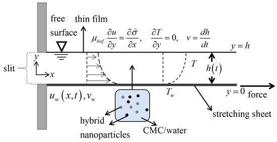
Figure 1.
Visual representation of the present flow problem over a stretching sheet.
Now, the Cross fluid’s Cauchy stress tensor is formulated as [29]
Here, is pressure, is the identity tensor, and is the rheology equation for viscosity in respect to shear rate, which is conveyed as follows [29]:
wherein and are the high and low shear rates restricting viscosities, respectively; is the power-law index, and it is a non-dimensional constant; signifies the material time constant; is the shear rate; and is the first Rivlin–Ericksen tensor. and can be further elaborated as follows [29]:
Next, must be fixed to be zero, and hence (3) becomes [30]
Moreover, is determined by choosing the velocity and temperature fields in a manner, where
and thus
The Cross model reveals the pseudoplastic feature when the power-law index is within the values of zero and one. The Cross model exhibits the dilatant characteristic when is more than 1, while setting and equal to zero reduces the Cross model into a Newtonian model. Under these assumptions, the governing unsteady liquid film flow of the Cross hybrid nanofluid past the stretching surface can be written as [29]
conditional on the following boundary constraints:
where is the surface tension which varies linearly with temperature [20] while the nanoparticles’ fluxes crossing the boundary at the free surface and at the stretching sheet are assumed to be zero [31]. Thus, can be expressed as [17]
where is the positive fluid property. The wall temperature is given as [17]
where denotes the slit temperature and represents the reference temperature, which can be chosen as a constant temperature difference. Meanwhile, the expression of as in (10) elucidates the depreciation of stretching sheet temperature from the slit temperature in proportion to [6]. The rate of temperature diminution past the stretching sheet increases with time [6]. The boundary condition in (12c) imposes a kinematic constraint of the fluid motion. Note that that the definition for and is only valid for time less than
The hybrid nanofluid’s dynamic viscosity, density, and thermal conductivity are denoted by and while the hybrid nanofluid’s heat capacity symbolized as The definition of and are given in Table 1. By referring to Table 1, the nanoparticle volume fraction is m and when is zero, the model is reduced into a regular fluid. Next, and signify Al2O3’s and Cu’s nanoparticle volume fractions, respectively.

Table 1.
The correlation properties of the Al2O3–Cu/H2O hybrid nanofluid can provide valuable insights into the behavior of the nanofluid. It is important to understand these properties to optimize the performance of the nanofluid in various applications. These correlations are adapted from Takabi and Salehi [32].
Meanwhile,
is the hybrid nanoparticle volume fraction. and are the densities of the base fluid and the hybrid nanoparticle, respectively; and are the thermal conductivities of the base fluid and the hybrid nanoparticles, respectively; and and are the heat capacitance of the base fluid and the hybrid nanoparticle, respectively. The range of is less than 0.05 [33]. The correlations in Table 1, which are correct and feasible, are based on physical assumptions and agree with the conservation of mass and energy. Table 2 provides the physical properties of the hybrid nanofluids used in the study, which include sodium carboxymethyl cellulose (CMC)/water, alumina (Al2O3), and copper (Cu). The non-Newtonian fluid, CMC/water, is created by combining an aqueous polymer solution of sodium carboxymethyl cellulose with water, and its mixing procedure has been previously described in experimental studies conducted by Zainith and Mishra [34], as well as Pinho and Whitelaw [35]. The heat transfer rate of the CMC/water-based nanofluid using alumina, titania, and copper nanoparticles has been shown to be higher than that of the conventional Newtonian fluid through experimental approaches by Hojjat et al. [36] and Zainith and Mishra [34], which demonstrates the potential of CMC/water-based nanofluid for enhancing heat transfer. As a result, the authors were motivated to investigate the effects of hybrid nanoparticles on the heat transfer rate and thin film thickness.
Table 2.
The thermophysical properties of selected nanoparticles and base fluid (sodium carboxymethyl cellulose(CMC)/water). The values presented in this table have been adapted from previous works by Oztop and Abu-Nada [37] as well as Abbas et al. [38].
Now, the similarity transformations from [6] are utilized as follows:
Here, the prime describes the derivative with respect to is an unknown parameter that communicates the dimensionless film thickness, and is the stream function. At the free surface, fix to 1 and Equation (16e) takes the following form:
which eventually gives
By employing the similarity conversion as in Equations (16a)–(16e) into the governing model, Equations (9)–(12c) satisfies the continuity equation, and the remaining equations are transformed as follows:
accompanied with the boundary conditions
while presenting the constant mass transfer parameter, , defined as with a setup where the suction effect appears with more than 0, while the injection situation occurs with less than 0. The local Weissenberg number, , is formulated as ; is an unknown constant to be calculated as a part of the problem defined as ; is the thermocapillarity number and defined as ; and is the dimensionless measure of unsteadiness that can be defined as Highlighted here is that setting to one and to zero impacts the model in Equations (19)–(21f), causing it to exhibit Newtonian characteristics.
On the other hand, the local skin friction coefficient and the local Nusselt number need to be formulated to encapsulate the present model’s transport phenomena behavior. Hence, and can be formulated as follows [19]:
wherein the wall shear stress and wall heat flux are denoted by and respectively, which can be elaborated further as [29]
Again, using the similarity transformations in Equations (16a)–(16e) facilitates the expressions in Equations (22)–(25) to obtain the following complete form of Equations (22) and (23) as follows:
Here, the Reynolds number is defined as follows:
3. Results and Discussion
This section presents the generated numerical results and clarifies the physical meaning behind the increasing or decreasing trends revealed by the physical quantities as the pertinent parameter values vary. The governing mathematical model in the form of the ordinary differential equations (see Equations (15)–(17)) is translated into the MATLAB bvp4c function code prior to the process of generating results. Generally, the MATLAB bvp4c function is a robust approach, and it was developed by Shampine et al. [39]. The bvp4c function is highly capable of identifying the approximate solutions for mathematical models with the presence of an unknown parameter; for an example, see Equations (15)–(17). The rule is simple, where the good-guess values for solving the respective mathematical model and obtaining the unknown parameter’s value must be accommodated in the code. While exercising the bvp4c routine for solving the present model, the relative tolerance has been fixed at to ensure all computed numerical solutions are accurate to within 0.001%. The hybrid nanofluid is implemented in the equations via the hybrid nanofluid correlation properties given in Table 1. In order to generate the numerical solutions for the hybrid nanofluid case, the hybrid nanoparticle volume fraction is fixed such as
Meanwhile, for the monotyped nanofluid case, the copper’s nanoparticle volume fraction is considered zero. Table 3 indicates the numerical results in agreement with the analytic solutions generated by Wang [6], hence validating the proficiency of the bvp4c routine in MATLAB.
Table 3.
By comparing the numerical values of when and Pr are equal to one and , and are equal to zero with those found in previous related studies, a better understanding can be gained.
Before moving forward with the presentation and explanations of results, it is vital to convey the governing parameters’ values implemented in this valuable study. Apart from the parameters associated with the hybrid nanofluids, in sum, six physical parameters are acting on this flow model as follows:
- the local Weissenberg number ,
- the power-law index ,
- the thermocapillarity parameter ,
- the unsteadiness parameter ,
- the constant mass transfer parameter is fixed at and
- the Prandtl number is fixed at 7 throughout the computation since CMC/water is the base fluid examined in the present work. The Prandtl number value is valid when 293.15 K.
Let us begin the discussions by analyzing the local Weissenberg number variation’s impact on the flow model’s transport phenomena. Collecting the reduced skin friction coefficient values from Table 4, it is clear that an increment in from 0 to 0.5 causes to decrease by about 19.44% for both cases of hybrid nanofluid and mono nanofluid. Typically, an increment in induces the fluid’s relaxation time to increase and eventually makes the fluid more resistant to flow. Thus, the fluid velocity decreases, reducing the wall shear stress and lessening on the accelerated sheet. The velocity profiles as varies are not included in the manuscript due to the insignificant variation among the profiles. However, a similar flow behavior has been reported by Naganthran et al. [27] and Hayat et al. [40]. Meanwhile, in terms of the heat energy progression of the present model, data in Table 4 show that the heat transfer rate or increases for both cases of the hybrid nanofluid and mono nanofluid when increases. It is worth mentioning that the negative sign indicates that the energy in the form of energy transmits from the hot surface of the accelerated sheet to the cool fluid flow regime. Next, in the attempt to expound the increment trend of along with the rise in , the temperature profiles’ behavior must be captured from Figure 2. Figure 2 illuminates that an increment in the local Weissenberg number has an increasing effect on the temperature profiles. As the fluid travels from the surface of the stretching sheet to the liquid thin film, an increment in causes the fluid to be more viscous and contributes to retarding the flow. Eventually, the fluid temperature increases, raising the surface heat flux of the stretching sheet, resulting in an increased heat transfer rate. Hence, the results, as reported in Figure 2, are in accordance with the reported heat transfer rates in Table 5. Furthermore, the increment in increases the liquid thin film thickness by about 88.34% regardless of mono-typed or hybrid nanofluid.
Table 4.
As the local Weissenberg number undergoes variation, numerical approximations are made for the values of both the dimensionless film thickness or and the local skin friction coefficient . These approximations are based on specific parameters including and .
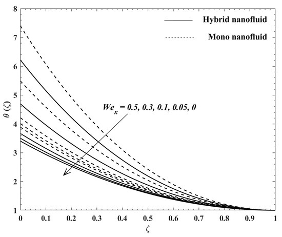
Figure 2.
Under the given conditions of , and the temperature profiles exhibit changes as varies. The variations in can result in significant changes in the temperature distribution, and the temperature profiles can provide valuable insights into the behavior of the system.
Table 5.
As the local Weissenberg number undergoes variation, numerical approximations are made for the local Nusselt number based on specific parameters, including , and .
The present theoretical model’s adequacy is further tested by varying the power-law index parameter or Interestingly, the increment in m from 0 to 1.6 conveys the variation in the Cross fluid from the Newtonian feature to shear thinning and, finally, to the shear thickening feature. These alteration of the fluid’s features from Newtonian and shear thinning to shear thickening causes the fluid to become more viscous when increases. Examining the numerical data from Table 6 makes it apparent that the changing flow feature of Cross fluid by increasing results in the diminution of the liquid film thickness at the rate of 48.95% for both cases of hybrid nanofluid or mono nanofluid. The lessening liquid film thickness increases the fluid velocity over the accelerated sheet. The fluid velocity increment causes the wall shear stress to increase, which then causes to increase. A similar trend result has been reported by Andersson et al. [10]. Meanwhile, according to Figure 3, an increment in reduces the fluid temperature, lowering the heat flux and declining the heat transfer rate on the sheet’s surface. Thus, Table 7 confirms the decrement trend of with the increasing trend of These are the consequences experienced by the present model when the fluid viscosity increases.
Table 6.
As the power-law index undergoes variation, numerical approximations are made for the values of both the dimensionless film thickness or , as well as the local skin friction coefficient, These approximations are based on specific parameters including , and .
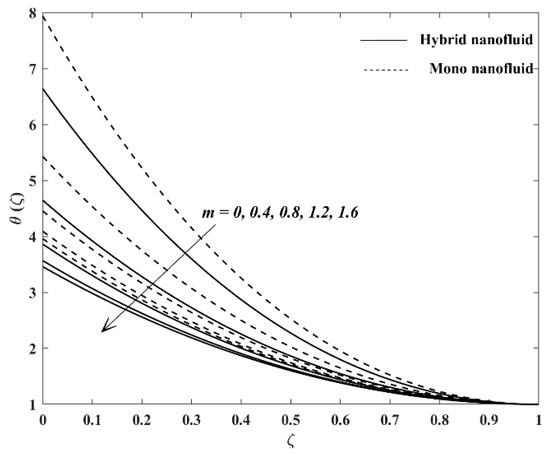
Figure 3.
Under the given conditions of , and the temperature profiles exhibit changes as varies. The variations in can result in significant changes in the temperature distribution, and the temperature profiles can provide valuable insights into the behavior of the system.
Table 7.
As the power-law index undergoes variation, numerical approximations are made for the local Nusselt number based on specific parameters, including , and .
Table 8 and Table 9, along with Figure 4 and Figure 5, display the changes experienced by the thin film flow model when the thermocapillarity parameter is adjusted from 0.3 to 1.9. The analysis of results begins with the dimensionless film thickness; there is an increasing trend for both cases of nanofluids when increases. An increase in generates surface-tension gradients within the flow regime, which produces the interfacial flow. This interfacial flow can arise either through viscous drag acting against the shear-driven motion caused by the accelerated surface or by assisting it. Table 8 proves that when the thin liquid film thickened because had an insignificant effect on the interfacial shear stress. Dandapat et al. [41] have reported that in the range of the film becomes thickened significantly. Table 8 shows that the thicker thin film formation reduces the fluid velocity and lowers the wall shear stress, resulting in low-resistance force exerted on the accelerating surface. Therefore, Table 8 conveys the decrement trend of when increases. Based on the generated velocity profiles in Figure 4, it is apparent that there is an insignificant difference between the hybrid and mono-typed nanofluids with respect to the changes in This can be explained with the definition of the thermocapillary number, Here, the nanofluid dynamic viscosity is dependent on the nanoparticle volume fractions in the base fluid. The increment in nanoparticle volume fractions raises fluid viscosity, suspending the fluid capability to flow [40]. Therefore, in the interfacial flow, the fluid velocity is insignificant among the hybrid nanofluid and mono-typed nanofluid.
Table 8.
As the thermocapillarity number undergoes variation, numerical approximations are made for the values of both the dimensionless film thickness or and the local skin friction coefficient, These approximations are based on specific parameters including , and .
Table 9.
As the thermocapillarity parameter undergoes variation, numerical approximations are made for the local Nusselt number based on specific parameters, including , and .
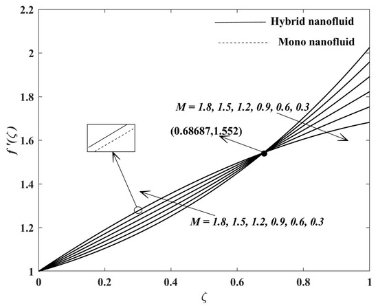
Figure 4.
When the values of and are held constant, the velocity profiles exhibit changes as varies. These variations can have a significant impact on the velocity distribution and provide valuable insights into the behavior of the system. Considering the correlation between the thermocapillarity parameter and the velocity profiles can aid in making well-informed decisions regarding the design and operation of the system.
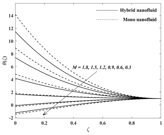
Figure 5.
Under the given conditions of , and , changes in the thermocapillarity parameter or cause variations in the temperature profiles. These changes in the can significantly affect the temperature distribution, and understanding the relationship between the thermocapillarity parameter and the temperature profiles can provide valuable insights into the system’s behavior.
Moreover, the behavior two distinct velocity profiles is evident as the boundary layer thickness increases from 0 to 1. The first region is when reflects the decrement in the flow velocity when increases. In contrast, the opposite trend has been identified in the second region, situated within the region , such that the flow velocity increases as M’s intensity rises from 0.3 to 1.8. These trends are also applicable to the dilatant state. The results suggest that there are two different mechanisms at play as the boundary layer thickness increases in the flow of hybrid nanofluids past an unsteady stretching sheet. In the first region, where the boundary layer thickness is relatively low, the thermocapillarity effect leads to a reduction in the flow velocity. This means that as the thermocapillarity number increases, the flow slows down. This is likely due to the fact that the thermocapillarity effect creates additional resistance to the flow, leading to a decrease in velocity. In the second region, where the boundary layer thickness is relatively high, the opposite trend is observed. Here, as the thermocapillarity number increases, the flow velocity actually increases. This suggests that in this region, the thermocapillarity effect is actually helping to promote the flow of the fluid. This may be due to the fact that the thermocapillarity effect creates a gradient in the surface tension of the fluid, which can help to drive the flow. It is best to highlight here that Dandapat et al. [41] and Aziz et al. [42] state that impacts the flow regime such that outward flow exists at the free surface without affecting the flow behavior at the accelerating sheet. Intriguingly, Table 7 shows that negative film thickness was reported when . The negative liquid film thickness indicates the rupture in the coating formation of the liquid film past the accelerated surface [19]. Figure 5 shows the temperature profiles when varies, and it is apparent that the fluid temperature rises as increases from 0.3 to 1.8. Moreover, as the fluid travels from the accelerated surface to the liquid thin film’s edge, the temperature drops (except for and 0.6). The rise in the surface tension at reduces the fluid temperature at . Meanwhile, at where the fluid is warm, an increase in increases the surface heat flux, which then increases the heat transfer rate at the stretching sheet. However, at low values of such that it is noticeable from Table 8 that the heat energy is transferred from the fluid flow regime to the accelerated sheet.
Finally, the present theoretical model is investigated in terms of the unsteadiness parameter and Table 10 shows that a gradual increment of from 0.1 to 1.5 reduces the liquid film thickness, and at negative film thickness is observed. On the other hand, the reduction in the film thickness speeds the fluid flow near the accelerating sheet (see Figure 6), causing to increase. Wang [6] also reported a similar trend when the intensity of was increased. Again, Figure 6 indicates an insignificant difference between the hybrid nanofluid and mono-typed nanofluid. Furthermore, in Table 11, an increment in was found to dissipate heat and lower the fluid temperature in the fluid regime (see Figure 7). Consequently, heat flux at the accelerating sheet is decreased and lowers the heat transfer rate on the accelerated sheet. It is suggested that the numerical results associated with the negative film thickness are omitted, that is, when , because the coating process has been disrupted. Overall, it is clear that the mono nanofluid is warmer than the hybrid nanofluid.
Table 10.
As the unsteadiness parameter undergoes variation, numerical approximations are made for the values of both the dimensionless film thickness or and the local skin friction coefficient These approximations are based on specific parameters including and .
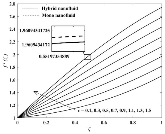
Figure 6.
Under the given conditions of , and , changes in the unsteadiness parameter cause variations in the velocity profiles. These variations can have a significant impact on the velocity distribution and provide valuable insights into the behavior of the system.
Table 11.
As the unsteadiness parameter undergoes variation, numerical approximations are made for the local Nusselt number, based on specific parameters, including , and .
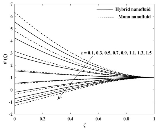
Figure 7.
Changes in the unsteadiness parameter or under the specified conditions of , and lead to variations in the temperature profiles. These variations can have a significant impact on the temperature distribution and provide valuable insights into the behavior of the system.
4. Conclusions
The present theoretical investigation provides new insights into the co-extrusion problem of the thin surface layer. The key results of the present work are as follows. The increasing trend of the local Weissenberg number and the thermocapillarity number showed a thicker liquid thin film, which then decreased the local skin friction coefficient over the stretching surface and heightened the heat transfer rate. The increasing trend of the power-law index and the unsteadiness parameter yielded the thinner liquid thin film, increased the local skin friction coefficient , and reduced the heat transfer rate. An increase in the local skin friction coefficient caused an increase in the drag force acting on the surface, which in turn increased the resistance to flow. This means that the fluid flow became more turbulent and the velocity gradient near the surface increased, leading to an increase in the shear stress acting on the surface. In practical applications, an increase in the skin friction coefficient can lead to increased energy losses, reduced efficiency, and increased wear and tear on the surface in contact with the fluid.
Negative film thickness is unfavorable and attainable when the unsteadiness parameter’s range is more than or equal to 0.9 and when the thermocapillarity parameter’s range is within the values of zero and 0.6. Additionally, from the perspective of the thin hybrid nanofluid and thin mono-typed nanofluid transport phenomena over an unsteady stretching sheet, it is understood that the fluid velocity is insignificant as the governing parameters vary and the mono-typed nanofluid is warmer than the hybrid nanofluid in the flow region. When the intensity of each governing parameter increases, several conclusions can be drawn. First, a thinner film is formed with a hybrid nanofluid compared to a mono-typed nanofluid. Second, the drag force on the constantly accelerating sheet is greater in the case of hybrid nanofluid film flow compared to mono-typed nanofluid film flow. Finally, the heat transfer rate on the constantly accelerating sheet is lower in the case of hybrid nanofluid film flow compared to mono-typed nanofluid film flow.
The future of the present work appears promising in several respects. Initially, one can expand the study to consider other varieties of nanofluids, such as the next generation of the nanofluid or ternary hybrid nanofluid to compare the results and detect any new phenomena. Subsequently, additional exploration can be conducted to examine the effect of diverse stretching parameters on the thermocapillary flow behavior of the hybrid nanofilm. Thirdly, the investigation can be extended to analyze the impact of magnetic fields, which have been identified to influence nanofluids’ flow characteristics significantly. Ultimately, the results of this research can optimize the performance and efficiency of various industrial applications, such as microfluidic devices, drug delivery systems, and nanofluidic heat transfer systems.
Author Contributions
Conceptualization, K.N., I.H. and R.N.; methodology, K.N.; software, K.N.; validation, K.N., I.H. and R.N.; writing—original draft preparation, K.N., D.A.J. and E.A.; writing—review and editing, D.A.J. and E.A.; supervision, R.N. and I.H.; project administration, R.N.; funding acquisition, R.N. All authors have read and agreed to the published version of the manuscript.
Funding
This research was funded by Malaysian Ministry of Higher Education, grant number FRGS/1/2020/STG06/UKM/01/1.
Institutional Review Board Statement
Not applicable.
Informed Consent Statement
Not applicable.
Data Availability Statement
Not applicable.
Acknowledgments
The authors would like to extend appreciation for the financial assistance provided by the Malaysian Ministry of Higher Education.
Conflicts of Interest
The authors declare no conflict of interest.
Nomenclature
| first Rivlin-Ericksen tensor | |
| Al2O3 | alumina |
| stretching rate | |
| local skin friction coefficient | |
| specific heat at constant pressure | |
| CMC | sodium carboxymethyl cellulose |
| Cu | copper |
| positive constant | |
| dimensionless stream function | |
| liquid thin film thickness | |
| identity tensor | |
| fluid’s thermal conductivity | |
| hybrid nanofluid’s thermal conductivity | |
| power-law index | |
| thermocapillarity number | |
| local Nusselt number | |
| pressure | |
| Pr | Prandtl number |
| wall heat flux | |
| unknown constant | |
| local Reynolds number | |
| constant mass transfer parameter | |
| temperature | |
| temperature at slit | |
| surface temperature | |
| reference temperature | |
| time | |
| velocity components at and axes | |
| velocity fields | |
| uniform surface mass flux | |
| local Weissenberg number | |
| Cartesian coordinates | |
| Greek symbols | |
| unknown parameter | |
| shear rate | |
| material time constant | |
| unsteadiness parameter | |
| similarity variable | |
| apparent viscosity | |
| high shear rates viscosity | |
| zero shear rates viscosity | |
| non-dimensional temperature | |
| hybrid nanofluid’s dynamic viscosity | |
| fluid’s dynamic viscosity | |
| base fluid’s kinematic viscosity | |
| hybrid nanofluid’s density | |
| surface tension | |
| surface temperature at | |
| Cauchy stress tensor | |
| wall shear stress | |
| Al2O3’s nanoparticle volume fraction | |
| Cu’s nanoparticle volume fraction | |
| hybrid nanoparticle volume fraction | |
| stream function | |
| positive fluid property | |
| Subscripts | |
| condition at the stretching sheet’s wall | |
| base fluid | |
| nanofluid | |
| hybrid nanofluid | |
| Al2O3’s solid component | |
| Cu’s solid component | |
| Superscript | |
| derivative with respect to | |
References
- Gil, M.; Rudy, M. Innovations in the packaging of meat and meat products—A review. Coatings 2023, 13, 333. [Google Scholar] [CrossRef]
- Barborik, T.; Zatloukal, M. Steady-state modeling of extrusion cast film process, neck-in phenomenon, and related experimental research: A review. Phys. Fluids 2020, 32, 061302. [Google Scholar] [CrossRef]
- Wang, C.Y. Liquid film on an unsteady stretching surface. Q. Appl. Math. 1990, 48, 601–610. [Google Scholar] [CrossRef]
- Usha, R.; Sridharan, R. The axisymmetric motion of a liquid film on an unsteady stretching surface. J. Fluids Eng. 1995, 117, 81–85. [Google Scholar] [CrossRef]
- Andersson, H.I.; Aarseth, J.B.; Dandapat, B.S. Heat transfer in a liquid film on an unsteady stretching surface. Int. J. Heat Mass Transf. 2000, 43, 69–74. [Google Scholar] [CrossRef]
- Wang, C. Analytic solutions for a liquid film on an unsteady stretching surface. Heat Mass Transf. 2006, 42, 759–766. [Google Scholar] [CrossRef]
- Noor, N.F.M.; Abdulaziz, O.; Hashim, I. MHD flow and heat transfer in a thin liquid film on an unsteady stretching sheet by the homotopy analysis method. Int. J. Numer. Methods Fluids 2010, 63, 357–373. [Google Scholar] [CrossRef]
- Khan, Y.; Wu, Q.; Faraz, N.; Yildirim, A. The effects of variable viscosity and thermal conductivity on a thin film flow over a shrinking/stretching sheet. Comput. Math. Appl. 2011, 61, 3391–3399. [Google Scholar] [CrossRef]
- Bird, R.B.; Armstrong, R.C.; Hassager, O. Dynamics of Polymeric Liquids, Volume 1: Fluid Mechanics, 2nd ed.; John Wiley & Sons: New York, NY, USA, 1987. [Google Scholar]
- Andersson, H.I.; Aarseth, J.B.; Braud, N.; Dandapat, B.S. Flow of a power-law fluid film on an unsteady stretching surface. J. Non-Newton. Fluid Mech. 1996, 62, 1–8. [Google Scholar] [CrossRef]
- Wang, C.; Pop, I. Analysis of the flow of a power-law fluid film on an unsteady stretching surface by means of homotopy analysis method. J. Non-Newton. Fluid Mech. 2006, 138, 161–172. [Google Scholar] [CrossRef]
- Chen, C.H. Heat transfer in a power-law fluid film over a unsteady stretching sheet. Heat Mass Transf. 2003, 39, 791–796. [Google Scholar] [CrossRef]
- Bilal, M.; Saeed, A.; Gul, T.; Rehman, M.; Khan, A. Thin-film flow of Carreau fluid over a stretching surface including the couple stress and uniform magnetic field. Partial Differ. Equ. Appl. Math. 2021, 4, 100162. [Google Scholar] [CrossRef]
- Naganthran, K.; Hashim, I.; Nazar, R. Non-uniqueness solutions for the thin Carreau film flow and heat transfer over an unsteady stretching sheet. Int. Commun. Heat Mass Transf. 2020, 117, 104776. [Google Scholar] [CrossRef]
- Cross, M.M. Rheology of non-Newtonian fluids: A new flow equation for pseudoplastic systems. J. Colloid Sci. 1965, 20, 417–437. [Google Scholar] [CrossRef]
- Khan, M.; Manzur, M. Boundary layer flow and heat transfer of Cross fluid over a stretching sheet. arXiv 2016. [Google Scholar] [CrossRef]
- Dandapat, B.S.; Santra, B.; Andersson, H.I. Thermocapillarity in a liquid film on an unsteady stretching surface. Int. J. Heat Mass Transf. 2003, 46, 3009–3015. [Google Scholar] [CrossRef]
- Chen, C.H. Marangoni effects on forced convection of power-law liquids in a thin film over a stretching surface. Phys. Lett. A 2007, 370, 51–57. [Google Scholar] [CrossRef]
- Naganthran, K.; Hashim, I.; Nazar, R. Triple solutions of Carreau thin film flow with thermocapillarity and injection on an unsteady stretching sheet. Energies 2020, 13, 3177. [Google Scholar] [CrossRef]
- Megahed, A.M.; Mahmoud, M.A.A. MHD non-Newtonian thin film fluid flow due to an unsteady stretching sheet under thermocapillarity phenomenon. Int. J. Mod. Phys. C 2019, 30, 1950085. [Google Scholar] [CrossRef]
- Choi, S.U.S.; Eastman, J.A. Enhancing thermal conductivity of fluids with nanoparticles. ASME Publ. FED 1995, 231, 99–103. [Google Scholar]
- Narayana, M.; Sibanda, P. Laminar flow of a nanoliquid film over an unsteady stretching sheet. Int. J. Heat Mass Transf. 2012, 55, 7552–7560. [Google Scholar] [CrossRef]
- Xu, H.; Pop, I.; You, X.C. Flow and heat transfer in a nano-liquid film over an unsteady stretching surface. Int. J. Heat Mass Transf. 2013, 60, 646–652. [Google Scholar] [CrossRef]
- Suresh, S.; Venkitaraj, K.P.; Selvakumar, P.; Chandrasekar, M. Synthesis of Al2O3-Cu/water hybrid nanofluids using two step method and its thermo physical properties. Colloids Surf. A Physicochem. Eng. Asp. 2011, 388, 41–48. [Google Scholar] [CrossRef]
- Sundar, L.S.; Singh, M.K.; Sousa, A.C.M. Enhanced heat transfer and friction factor of MWCNT-Fe3O4/water hybrid nanofluids. Int. Commun. Heat Mass Transf. 2014, 52, 73–83. [Google Scholar] [CrossRef]
- Devi, S.P.A.; Devi, S.S.U. Numerical investigation of hydromagnetic hybrid Cu-Al2O3/water nanofluid flow over a permeable stretching sheet with suction. Int. J. Nonlinear Sci. Numer. Simul. 2016, 17, 249–257. [Google Scholar] [CrossRef]
- Naganthran, K.; Nazar, R.; Siri, Z.; Hashim, I. Entropy Analysis and Melting Heat Transfer in the Carreau Thin Hybrid Nanofluid Film Flow. Mathematics 2021, 9, 3092. [Google Scholar] [CrossRef]
- Maity, S.; Ghatani, Y.; Dandapat, B.S. Thermocapillary flow of a thin nanoliquid film over an unsteady stretching sheet. J. Heat Transf. 2016, 138, 042401. [Google Scholar] [CrossRef]
- Azam, M.; Shakoor, A.; Rasool, H.F.; Khan, M. Numerical simulation for solar energy aspects on unsteady convective flow of MHD Cross nanofluid: A revised approach. Int. J. Heat Mass Transf. 2019, 131, 495–505. [Google Scholar] [CrossRef]
- Boger, D.V. Demonstration of upper and lower Newtonian fluid behaviour in a pseudoplastic fluid. Nature 1977, 265, 126–128. [Google Scholar] [CrossRef]
- Abdullah, A.A.; Lindsay, K.A. Marangoni convection in a thin layer of nanofluid: Application to combinations of water or ethanol with nanoparticles of alumina or multi-walled carbon nanotubules. Int. J. Heat Mass Transf. 2017, 104, 693–702. [Google Scholar] [CrossRef]
- Takabi, B.; Salehi, S. Augmentation of the heat transfer performance of a sinusoidal corrugated enclosure by employing hybrid nanofluid. Adv. Mech. Eng. 2014, 6, 147059. [Google Scholar] [CrossRef]
- Myers, T.G.; Ribera, H.; Cregan, V. Does mathematics contribute to the nanofluid debate? Int. J. Heat Mass Transf. 2017, 111, 279–288. [Google Scholar] [CrossRef]
- Zainith, P.; Mishra, N.K. Experimental and numerical investigations on exergy and second law efficiency of shell and helical coil heat exchanger using carboxymethyl cellulose based non-newtonian nanofluids. Int. J. Thermophys. 2022, 43, 3. [Google Scholar] [CrossRef]
- Pinho, F.T.; Whitelaw, J.H. Flow of non-Newtonian fluids in a pipe. J. Non-Newton. Fluid Mech. 1990, 34, 129–144. [Google Scholar] [CrossRef]
- Hojjat, M.; Etemad, S.G.; Bagheri, R. Laminar heat transfer of non-Newtonian nanofluids in a circular tube. Korean J. Chem. Eng. 2010, 27, 1391–1396. [Google Scholar] [CrossRef]
- Oztop, H.F.; Abu-Nada, E. Numerical study of natural convection in partially heated rectangular enclosures filled with nanofluids. Int. J. Heat Fluid Flow 2008, 29, 1326–1336. [Google Scholar] [CrossRef]
- Abbas, I.; Hasnain, S.; Alatawi, N.A.; Saqib, M.; Mashat, D.S. Non-Newtonian nano-fluids in Blasius and Sakiadis flows influenced by magnetic field. Nanomaterials 2022, 12, 4254. [Google Scholar] [CrossRef]
- Shampine, L.F.; Gladwell, I.; Thompson, S. Solving ODEs with MATLAB; Cambridge University Press: New York, NY, USA, 2003; p. 166. [Google Scholar]
- Hayat, T.; Khan, M.I.; Tamoor, M.; Waqas, M.; Alsaedi, A. Numerical simulation of heat transfer in MHD stagnation point flow of Cross fluid model towards a stretched surface. Results Phys. 2017, 7, 1824–1827. [Google Scholar] [CrossRef]
- Dandapat, B.S.; Santra, B.; Vajravelu, K. The effects of variable fluid properties and thermocapillarity on the flow of a thin film on an unsteady stretching sheet. Int. J. Heat Mass Transf. 2007, 50, 991–996. [Google Scholar] [CrossRef]
- Aziz, R.C.; Hashim, I.; Abbasbandy, S. Effects of thermocapillarity and thermal radiation on flow and heat transfer in a thin 583 liquid film on an unsteady stretching sheet. Math. Probl. Eng. 2012, 2012, 127320. [Google Scholar] [CrossRef]


Disclaimer/Publisher’s Note: The statements, opinions and data contained in all publications are solely those of the individual author(s) and contributor(s) and not of MDPI and/or the editor(s). MDPI and/or the editor(s) disclaim responsibility for any injury to people or property resulting from any ideas, methods, instructions or products referred to in the content. |
© 2023 by the authors. Licensee MDPI, Basel, Switzerland. This article is an open access article distributed under the terms and conditions of the Creative Commons Attribution (CC BY) license (https://creativecommons.org/licenses/by/4.0/).