Structural Fault Diagnosis Based on Static and Dynamic Response Parameters

Abstract

Structural fault diagnosis is an important subject for ensuring the normal use of structures. More test data will help to improve the accuracy and reliability of structural fault diagnosis. Therefore, a structural fault detection algorithm based on static–dynamic mixed sensitivity analysis is proposed. The vibration parameters used were the vibration modes of some of the nodes in the structure measured by the vibration test system. The static response parameter used was the vertical displacement of the structure under the gravity load measured by the static test system. In particular, the gravity load and the structure were connected rigidly to form a new added-mass system. The vibration mode of the additional-mass system was measured again to obtain more equations for fault evaluation. Based on the static and dynamic measurement data, the failure coefficients of all components in the structure were calculated through the mixed sensitivity of the static displacement and vibration-mode shape. According to the calculated value of the failure coefficient, the failure state of all components in the structure could be finally evaluated. The main innovation of the proposed method was the use of the static load as a part of the new added-mass system to obtain more vibration parameters for the defect diagnosis. The implementation process and effect of this method were verified using a numerical truss structure and an experimental steel beam structure. Moreover, the defect diagnosis results of the proposed hybrid method were compared with those of a pure static algorithm and a pure dynamic algorithm to illustrate the advantages of the hybrid method. The research results showed that this method has the advantages of simple implementation and high diagnosis accuracy. Especially for symmetric structures, the proposed method can successfully avoid the possible missed diagnoses of the pure static algorithm and pure dynamic method. The algorithm provides a simple and feasible method for structural defect identification.

1. Introduction

A structure will inevitably have faults due to the influence of environmental corrosion, material fatigue, disaster load, and so on. A fault in a structure will lead to a change in the structure’s response parameters under a static or dynamic load [1,2,3]. In practice, the static displacement of a structure can be measured through an optical system, and the vibration modal data of a structure can be tested by a vibration test system. Therefore, the fault condition of a structure can be evaluated according to a change in the static or dynamic parameters. In recent decades, a lot of research has been carried out on structural fault diagnosis. These fault diagnosis methods can generally be divided into static methods and dynamic methods. Static methods use the change in the static displacement or strain of a structure to evaluate the state of the structural faults. Using flexibility disassembly perturbation, Yang and Sun [4,5,6] proposed a fast analysis method for the static displacement for structural damage detection. Using the static strain change, Yang et al. [7] developed a model-free method for damage localization for a grid structure. Bakhtiari-Nejad et al. [8] developed non-linear equations that relate static response variations to fault location and extent. Abdo [9] established a relationship between the structural fault characteristics and displacement curvature variations. Tian et al. [10] carried out fault diagnosis on a wind turbine blade using the static strain responses of the fiber Bragg grating. Using static testing data, Santos et al. [11] detected faults in stay cables using statistical and machine-learning methods. Viola and Bocchini [12] developed a fault diagnosis technique for truss structures based on static load tests. Using structural optimization concepts, Terlaje et al. [13] proposed a parameter identification method to accurately assess the stiffness in linear elastic models of civil structures. Boumechra [14] used a bridge’s deflection under a moving load to determine the possible faults in the bridge’s structure. Based on static displacement, Peng et al. [15] developed a method for determining the damage location in a beam’s structure by using the redistribution of static shear energy. Chrysanidis [16] studied the main factors that affect the cracking of reinforced concrete columns and walls, such as load, tensile strain, etc. Based on the experimental results, the ranges, sizes, and locations of cracks in these components were summarized. The above research has shown the potential of static methods in diagnosing faults in beam-type structures. Dynamic methods use changes in structural vibration parameters, especially modal data, to evaluate the state of structural faults. Lu and Law [17] studied the sensitivity of dynamic parameters and proposed a sensitivity-based algorithm to detect faults in a structure. Feng [18] reported the applications of computer visions in structural modal parameter identification, model updating, fault diagnosis, and cable force estimation. Gentile et al. [19] proposed a dynamic-based technique for the continuous health monitoring of the tallest historic tower in Mantua, Italy. Almeida et al. [20] developed a fault diagnosis approach by considering both the time and frequency responses of structural dynamic responses. Yang et al. [21,22] studied a dynamic model reduction and carried out fault diagnosis using modal sensitivity based on a reduced model. Peng et al. [23] developed a dynamic flexibility method for fault diagnosis in steel truss structures. Weng et al. [24] reviewed dynamic sub-structuring methods for model correction and fault diagnosis in large-scale structures. Meixedo et al. [25] developed an unsupervised automatic data-driven methodology for detecting damage in railway bridges based on traffic-induced dynamic responses. These studies have shown the advantages of dynamic methods in damage diagnosis, without affecting the normal use of a structure.

Although significant progress has been made in fault diagnosis, there are still some challenges that need to be further addressed. The disadvantage of pure static methods is that some members in a structure may not be sensitive to vertical loading. Thus, it is difficult to diagnose the defect condition of these members using a pure static method since conventional static loading is carried out by gravity. For pure dynamic methods, a similar limitation exists since the faults in some components of a structure may not cause significant changes in the structural vibration parameters. Especially for symmetric structures, pure dynamic methods may lead to the misjudgment of defects because the damages in the symmetrical components may lead to similar changes in the vibration parameters. In view of this, a fault diagnosis technique based on static and dynamic hybrid measurements is more reliable in engineering applications since the missed diagnosis problem for symmetrical structures can be overcome by asymmetric gravity loading. For this purpose, a combination of static displacement and mode-shape sensitivities are employed in this work to calculate the damage parameters of all the components of a structure. The fault state of each component in a structure can be subsequently evaluated according to the calculation results. In addition, more test data will help to improve the accuracy and reliability of structural fault diagnosis. As a by-product of static loading, the gravity load and the structure can be connected rigidly to form a new added-mass system. The vibration mode of the added-mass system can be measured again so that more equations can be obtained for the fault evaluation. Combined with all static and dynamic test data, the proposed hybrid sensitivity method can obtain more accurate and reliable defect diagnosis results. The greatest innovation of the proposed method its use of static loading as a new added-mass system to obtain more vibration parameters for defect diagnosis. A steel roof truss structure was used to illustrate the implementation process and feasibility of this hybrid sensitivity method. It was shown that the proposed method can successfully avoid the possible missed diagnoses of pure static algorithms and pure dynamic methods. The results showed the potential application value of the proposed method in engineering applications. The framework of this article is as follows: Section 2 provides a detailed explanation of the calculation formula and operation process of the proposed hybrid sensitivity method. In Section 3, the proposed method is validated using a numerical model of a truss structure. In Section 4, an experimental beam is used to further verify the proposed approach. Section 5 presents the main conclusions of this work.

2. The Hybrid Sensitivity Method for Structural Fault Diagnosis

As stated before, some component faults in a structure are only sensitive to gravity loading and some component faults are only sensitive to structural vibration. Therefore, using a hybrid algorithm based on static and dynamic measurements to diagnose faults in a structure will be a more reliable method. To this end, a hybrid sensitivity method based on static and dynamic test data was developed to evaluate the fault states in a structure. The main formulas of this method were derived as follows.

2.1. Static Displacement Sensitivity

Static displacement is the most commonly used response parameter for structural defect diagnosis. In practice, static displacement can be measured using devices such as a dial gauge, a wire displacement gauge, or an optical system. The static displacement sensitivity formulas were derived to establish the relationship between the structural defect parameters and the static displacement changes. For a structure with and without faults, the static displacement under the gravity load vector $f$ can be obtained from the finite element model (FEM) by:

$$S_u{d}_u=f,$$

(1)

$$S_d{d}_d=f,$$

(2)

$$S_d=S_u-\Delta S,\mathrm{and}$$

(3)

$$d_d=d_u+\Delta d,$$

(4)

where $S_u$ is the stiffness matrix of the intact structure, $d_u$ is the displacement vector under the load $f$, $S_d$ is the stiffness matrix of the structure with faults, $d_d$ is the corresponding displacement vector, and $\Delta S$ and $\Delta d$ are the variations in the stiffness matrix and the displacement due to the faults. From Equations (1)–(4), we can obtain

$$S_u{d}_u+S_u\Delta d-\Delta S{d}_u-\Delta S\Delta d=f.$$

(5)

Equation (5) can be approximately rewritten as

$$S_u\Delta d=\Delta S{d}_u.$$

(6)

Using Equations (1) and (6), we can obtain

$$S_u\Delta d=\Delta S{S}_u^{-1}f.$$

(7)

From Equation (7), the displacement variation $\Delta d$ can be expressed as

$$\Delta d=S_u^{-1}\Delta S{S}_u^{-1}f.$$

(8)

According to FEM theory, the variation $\Delta S$ in the stiffness matrix can be written as the sum of the elementary stiffness matrix multiplied by a fault coefficient, that is:

$$\Delta S={\displaystyle \sum _{i=1}^N{\epsilon }_i}{S}_i,({\epsilon }_i\subset [0,1]),$$

(9)

where $S_i$ and ${\epsilon }_i$ are the $i$-th elementary stiffness matrix and the fault coefficient in the structure and $N$ is the number of elements in the structural FEM. Using Equation (9), Equation (8) can be further expressed as

$$\Delta d={\displaystyle \sum _{i=1}^N{\epsilon }_i}{\xi }_i\mathrm{and}$$

(10)

$${\xi }_i=S_u^{-1}{S}_i{S}_u^{-1}f,$$

(11)

where ${\xi }_i$ is called as the displacement sensitivity vector of the $i$-th element.

2.2. Vibration Mode Sensitivity

Vibration modes are the most commonly used dynamic parameters for structural defect diagnosis. In practice, vibration modes can be measured using accelerometers and spectrum analysis software. The vibration mode sensitivity formulas were derived to establish the relationship between the structural defect parameters and the vibration mode changes. It is known that the free vibration modes of an intact structure can be obtained by solving the following generalized eigenvalue equations:

$$(S_u-{\lambda }_{r}M){\phi }_r=0\mathrm{and}$$

(12)

$${\phi }_r^{T}M{\phi }_r=1,$$

(13)

where ${\lambda }_r$ and ${\phi }_r$ are the $r$-th eigenvalue and mode shape of structural free vibration, respectively, and $M$ is the mass matrix of the structural FEM. Generally, $M$ remains unchanged for a structure before and after damage. By taking the partial derivative of Equation (12) with respect to ${\epsilon }_i$, we can obtain

$$(S_u-{\lambda }_{r}M)\frac{\partial {\phi }_r}{\partial {\epsilon }_i}=(\frac{\partial {\lambda }_r}{\partial {\epsilon }_i}M-S_i){\phi }_r,$$

(14)

where $\frac{\partial {\lambda }_r}{\partial {\epsilon }_i}$ and $\frac{\partial {\phi }_r}{\partial {\epsilon }_i}$ are the first-order eigenvalue and mode shape sensitivities, respectively. According to the FEM theory, $S_u$ and $M$ are both symmetric matrices. From Equation (12), we can also obtain

$${\phi }_r^T(S_u-{\lambda }_{r}M)=0.$$

(15)

Using Equations (14) and (15), the eigenvalue sensitivity can be obtained by multiplying Equation (14) by ${\phi }_r^T$, as follows:

$$\frac{\partial {\lambda }_r}{\partial {\epsilon }_i}={\phi }_r^T{S}_i{\phi }_r.$$

(16)

The mode shape sensitivity $\frac{\partial {\phi }_r}{\partial {\epsilon }_i}$ can be calculated using the formula proposed by Yang et al. [26], as follows:

$$\frac{\partial {\phi }_r}{\partial {\epsilon }_i}={\Theta }^{-1}\Omega {\phi }_r,$$

(17)

$$\Omega =\frac{\partial {\lambda }_r}{\partial {\epsilon }_i}M-S_i,\mathrm{and}$$

(18)

$$\Theta =S_u-{\lambda }_{r}M+{\lambda }_r{\phi }_r{\phi }_r^{T}M.$$

(19)

If we assume that ${\phi }_{d,r}$ is the measured mode shape of a damaged structure, due to the faults in the structure, the mode shape variation $\Delta {\phi }_r$ can be obtained using

$$\Delta {\phi }_r={\phi }_{d,r}-{\phi }_r.$$

(20)

On the other hand, $\Delta {\phi }_r$ can be approximated using Taylor’s series expansion, as follows:

$$\Delta {\phi }_r={\displaystyle \sum _{i=1}^N{\epsilon }_i\frac{\partial {\phi }_r}{\partial {\epsilon }_i}}$$

(21)

2.3. The Hybrid Sensitivity

As stated before, more test data will help to improve the accuracy and reliability of structural fault diagnosis. As a by-product of static loading, the gravity load and the structure can be connected rigidly to form a new added-mass system. We can measure the vibration mode of the added-mass system again so that more modal equations can be obtained for the fault evaluation, if necessary. Similar to Equation (21), the mode shape sensitivity equation of the additional-mass system with the gravity load is

$$\Delta {\phi }_r^a={\displaystyle \sum _{i=1}^N{\epsilon }_i\frac{\partial {\phi }_r^a}{\partial {\epsilon }_i}},$$

(22)

where $\Delta {\phi }_r^a$ denotes the change of the $r$-th mode shape of the additional-mass system with the gravity load. The mode shape sensitivity $\frac{\partial {\phi }_r^a}{\partial {\epsilon }_i}$ of the added-mass system can be calculated by

$$\frac{\partial {\phi }_r^a}{\partial {\epsilon }_i}={\Theta }_a^{-1}{\Omega }_a{\phi }_r^a,$$

(23)

$${\Omega }_a=\frac{\partial {\lambda }_r^a}{\partial {\epsilon }_i}{M}_a-S_i,$$

(24)

$${\Theta }_a=S_u-{\lambda }_r^a{M}_a+{\lambda }_r^a{\phi }_r^a{({\phi }_r^a)}^T{M}_a,$$

(25)

$$\frac{\partial {\lambda }_r^a}{\partial {\epsilon }_i}={({\phi }_r^a)}^T{S}_i{\phi }_r^a,\mathrm{and}$$

(26)

$$M_a=M+D(f),$$

(27)

where $D(f)$ represents a diagonal matrix whose diagonal element is the mass corresponding to the load vector $f$. Finally, Equations (10), (21), and (22) can be combined to construct the hybrid sensitivity system, as follows:

$$\Delta p=\Pi \cdot \alpha ,$$

(28)

$$\Delta p=\left\{\begin{array}{c}\Delta d\\ \Delta {\phi }_r\\ \Delta {\phi }_r^a\end{array}\right\},$$

(29)

$$\Pi =\left[\begin{array}{ccc}{\xi }_1& \cdots & {\xi }_N\\ \frac{\partial {\phi }_r}{\partial {\epsilon }_1}& \cdots & \frac{\partial {\phi }_r}{\partial {\epsilon }_N}\\ \frac{\partial {\phi }_r^a}{\partial {\epsilon }_1}& \cdots & \frac{\partial {\phi }_r^a}{\partial {\epsilon }_N}\end{array}\right],\mathrm{and}$$

(30)

$$\alpha ={({\epsilon }_1,\cdots ,{\epsilon }_N)}^T.$$

(31)

From Equation (28), the fault coefficient ${\epsilon }_i$($i=1~N$) can be calculated by

$$\alpha ={\Pi }^{+}\Delta p.$$

(32)

We note that the linear approximation was adopted in the above sensitivity analysis. Reference [27] discusses the influence of the linear approximation on fault diagnosis results. It was found that the fault coefficients calculated from the linear approximation equations are always larger than the true values. When the degree of damage is severe, this error caused by the linear approximation cannot be ignored. The research results of Reference [27] found that 0.176 is the critical value for considering this error. For damage parameters with a calculated value greater than 0.176, another correction operation must be performed. The formula of the correction operation for those calculated fault coefficient values greater than 0.176 is

$${\epsilon }_i^a=\frac{{\epsilon }_i}{1+{\epsilon }_i}.$$

(33)

Thus far, the fault condition of all components in a structure can be evaluated based on the calculation results ${\epsilon }_i$ and ${\epsilon }_i^a$. Figure 1 shows the flow chart of the entire technique to explain the process more clearly.

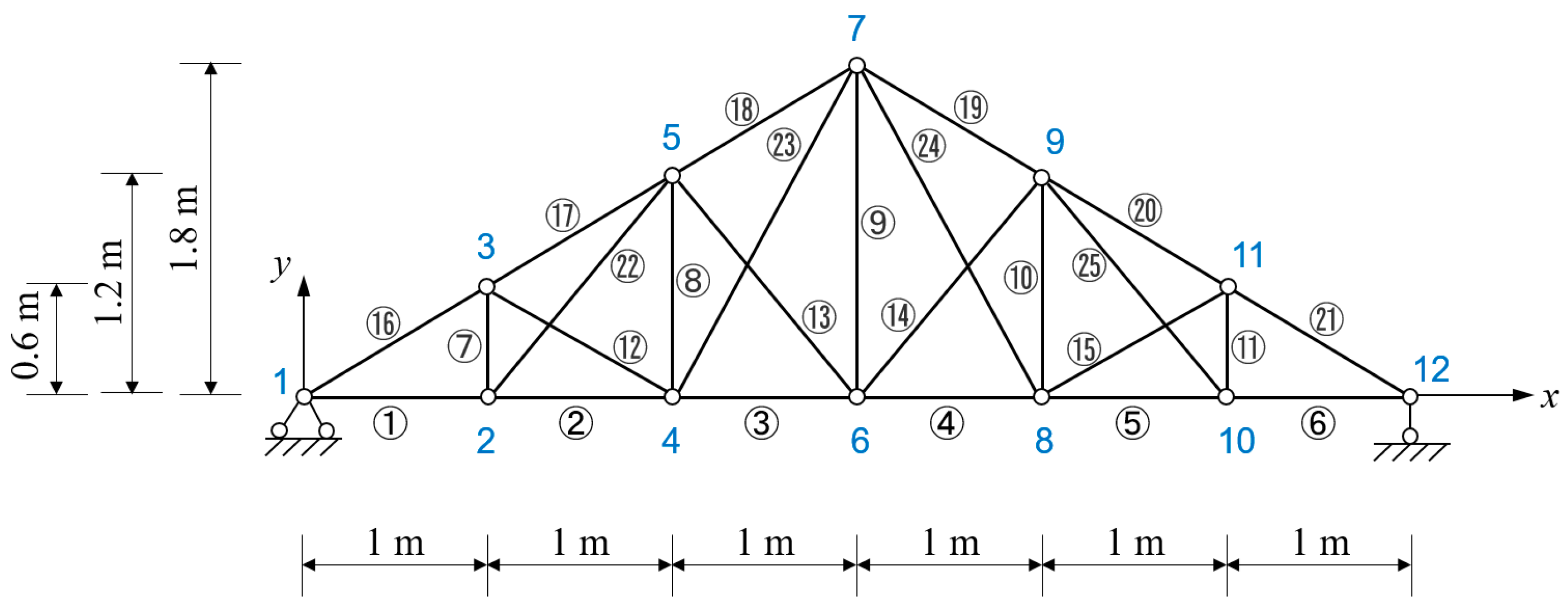
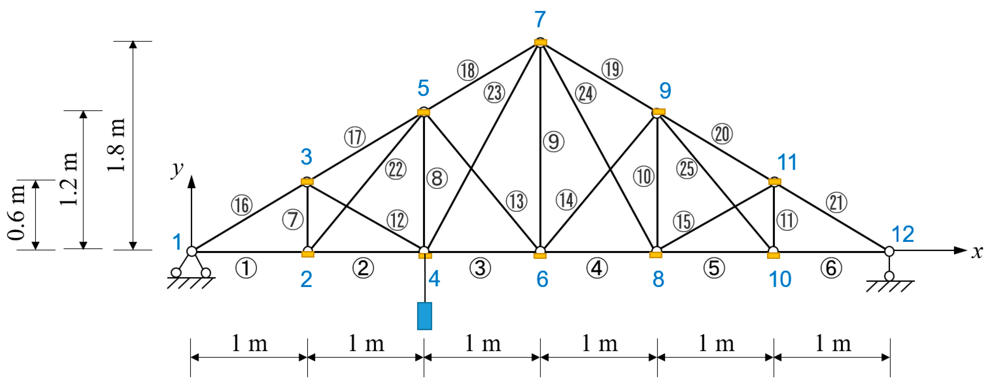
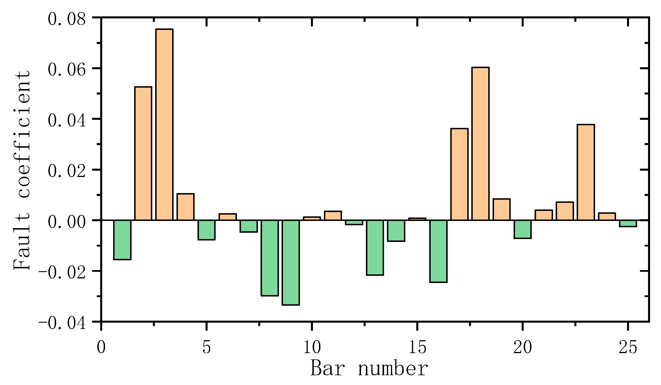
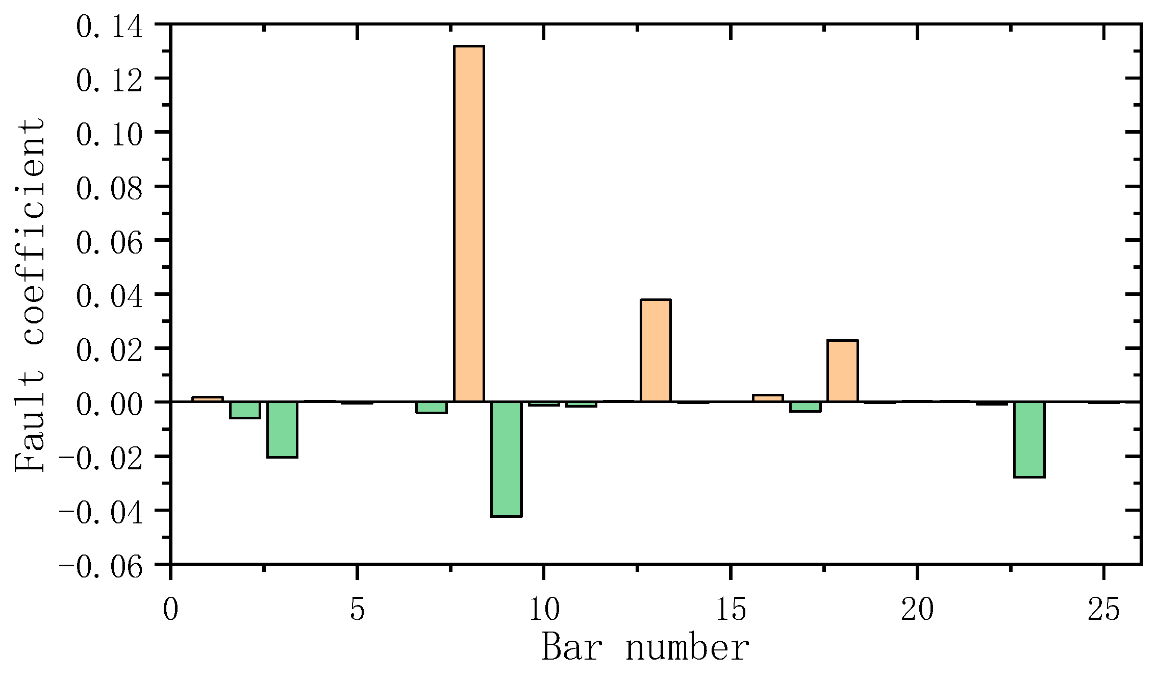
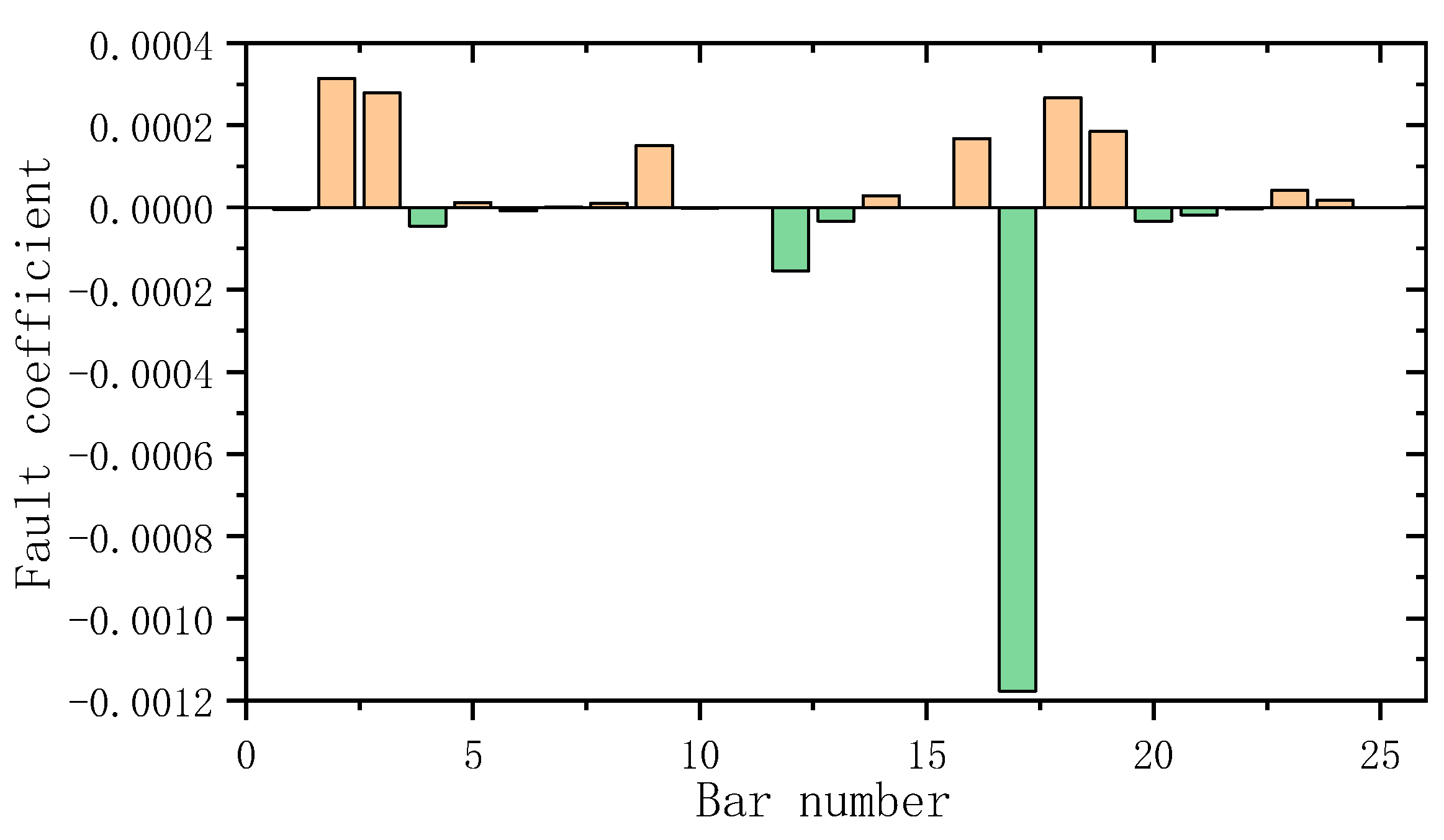
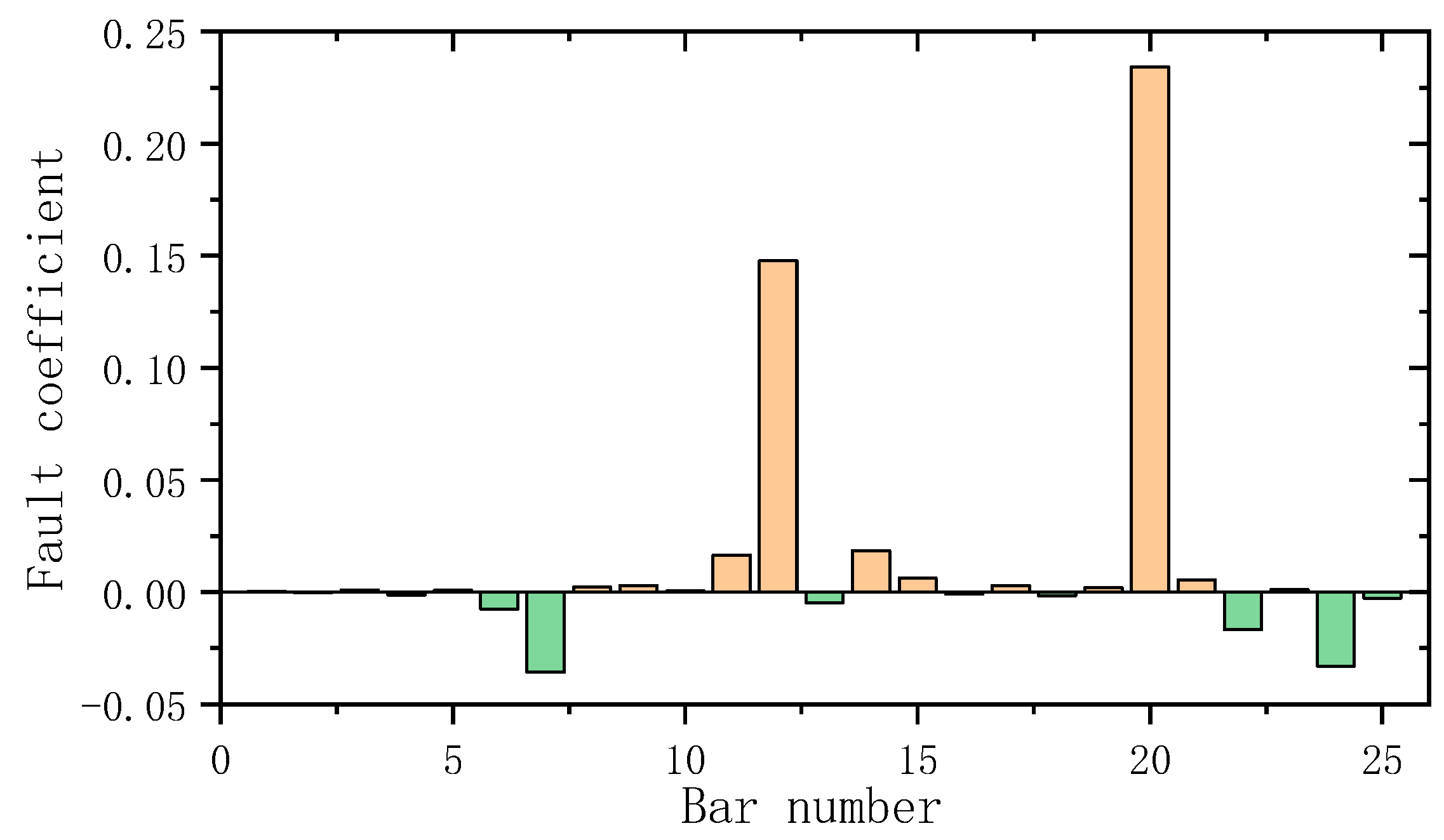
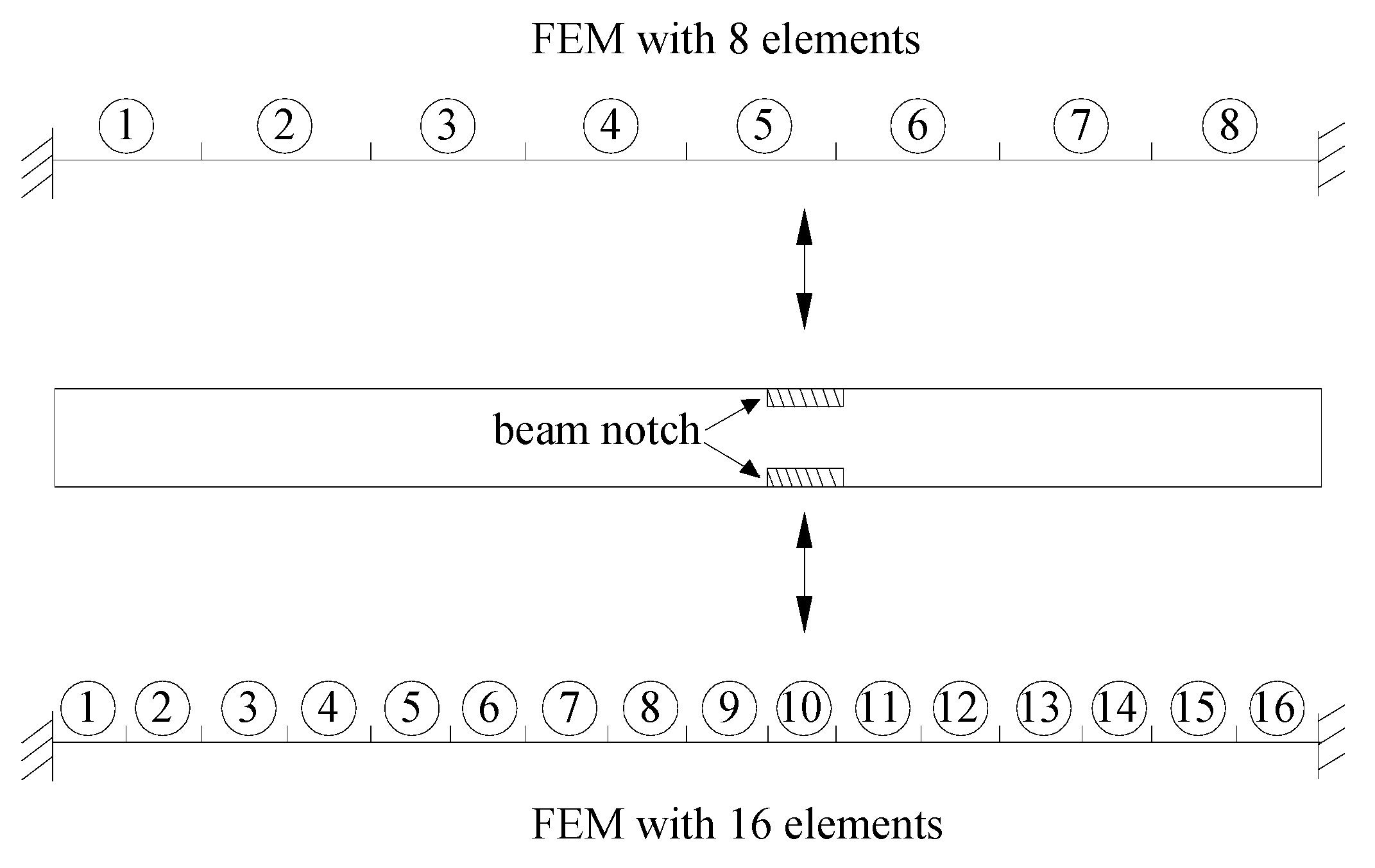
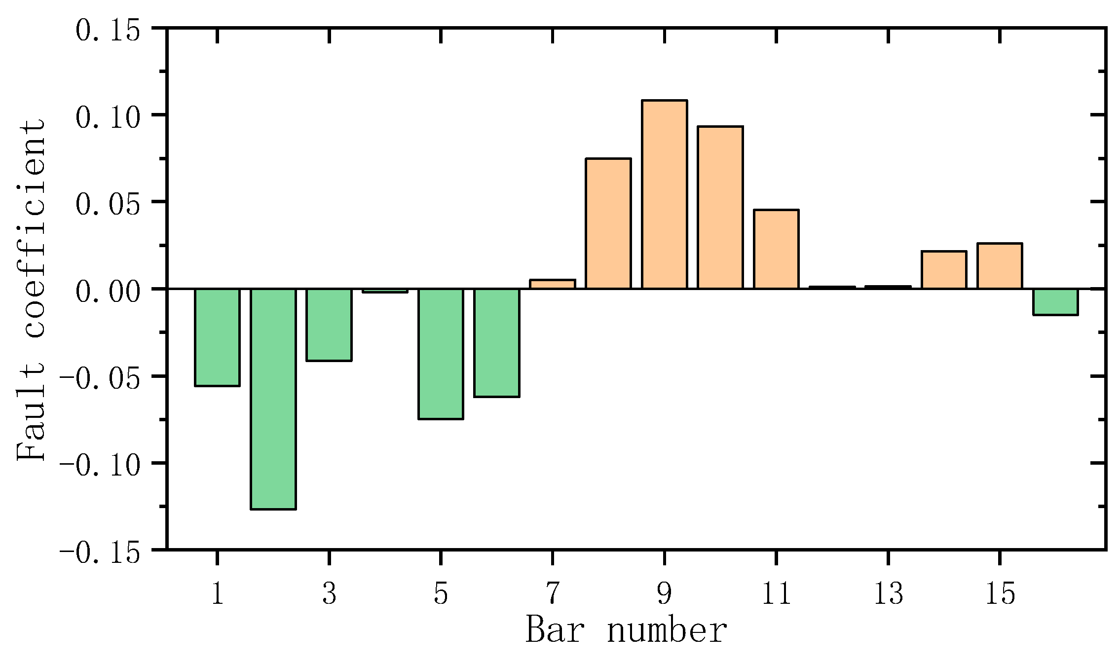
3. Numerical Example

As presented in Figure 2, the hybrid sensitivity method is illustrated by a steel roof truss structure with 25 bar elements. Note that the number in the circle in Figure 2 denotes the bar number in the FEM. We note that the connections of the bar elements were pin-jointed connections at all joints. The diagonal elements making an X-shape were not connected or truncated at the intersection points. Obviously, this structure could basically be regarded as a geometrically symmetric structure. The main physical parameters of the structure were as follows: the elastic modulus was 200 GPa, the density was 7800 kg/m³, and the cross-sectional area of each bar was 2.109 × 10⁻⁴ m².

As stated before, the asymmetric gravity loading can overcome the possible missed diagnosis problem in the diagnosis of symmetrical structural defects. For this purpose, the gravity loading, as shown in Figure 3, applied a concentrated force of 20 kN at node 4 in the structure. The number in the circle in Figure 3 denotes the bar number in the FEM. As a by-product of static loading, the gravity load and the structure were assumed to be connected rigidly to form a new added-mass system. In the static test, the vertical displacements of nodes 2–11 were observed through the optical measurement system. In the dynamic test, the horizontal accelerations of nodes 2–11 were observed through the vibration test system. We assumed that the accelerometers were arranged in the horizontal direction of nodes 2–11 to extract the vibration mode data in the horizontal direction. Figure 3 also provides the layout points marked in yellow for the acceleration sensors in the dynamic test. In the next numerical experiment, the fault in the structure was simulated by reducing the elastic modulus of some bar elements. The measured static and dynamic data were simulated from the FEMs of the undamaged and damaged structure.

The first defect case assumed that the elastic modulus of bar element 3 was reduced by 20%. Figure 4, Figure 5 and Figure 6 present the calculation results of the fault coefficients using a pure static algorithm, a pure dynamic algorithm, and the proposed hybrid method, respectively. We note that the pure static algorithm computed the fault coefficients using Equation (10) with only static data. The pure dynamic algorithm computed the fault coefficients using Equation (21) with only dynamic data. From Figure 4, Figure 5 and Figure 6, one can find that the fault coefficients obtained by the hybrid method more clearly indicated that the fault was located in bar element 3. Specifically, the fault extents obtained by the pure static method, the pure dynamic method, and the hybrid method were 7.5%, 18.4%, and 19.6%, respectively. Obviously, the fault extent (19.6%) calculated by the hybrid method was the closest to the assumed value (20%). It showed that the diagnosis result of the proposed method was the most reliable and accurate.

The second defect case assumed that the elastic modulus of bar element 8 was reduced by 15%. Figure 7, Figure 8 and Figure 9 present the calculation results of the fault coefficients using a pure static algorithm, a pure dynamic algorithm, and the proposed hybrid method, respectively. As seen in Figure 8, the pure dynamic method missed the diagnosis because it did not indicate that the defect was located in bar element 8. By comparing Figure 7 to Figure 9, one can find that the fault coefficients obtained by the hybrid method more clearly indicated that the fault was located in bar element 8. Specifically, the fault extents obtained by the pure static method, the pure dynamic method, and the hybrid method were 13.2%, 0%, and 15.2%, respectively. Clearly, the fault extent (15.2%) calculated by the hybrid method was the closest to the assumed value (15%). This showed again that the diagnosis result of the proposed method was the most reliable and accurate.

The third defect case assumed that the elastic moduli of bar elements 12 and 20 were reduced by 15% and 20%, respectively. Figure 10, Figure 11 and Figure 12 present the calculation results for this fault case using a pure static algorithm, a pure dynamic algorithm, and the proposed hybrid method, respectively. From Figure 10, Figure 11 and Figure 12, one can find that only the fault coefficients obtained using the hybrid method could clearly indicate that the faults were located in bar elements 12 and 20. Both the pure static method and the pure dynamic method could only indicate that there was defect in bar 20 and the fault in bar 12 was missed. Specifically, the fault extents of element 12 obtained by the pure static method, the pure dynamic method, and the hybrid method were 0%, 0.2%, and 14.8%, respectively. The fault extents of element 20 obtained by the pure static method, the pure dynamic method, and the hybrid method were 16.4%, 17.3%, and 19%, respectively. Clearly, the fault extents (14.8% and 19%) obtained by the proposed hybrid method were the closest to the assumed values (15% and 20%). These results showed that the proposed method did not miss diagnosis and had high calculation accuracy.

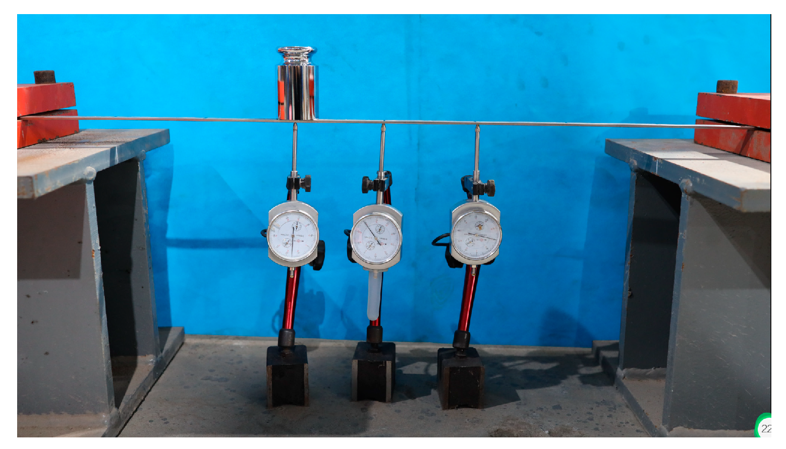
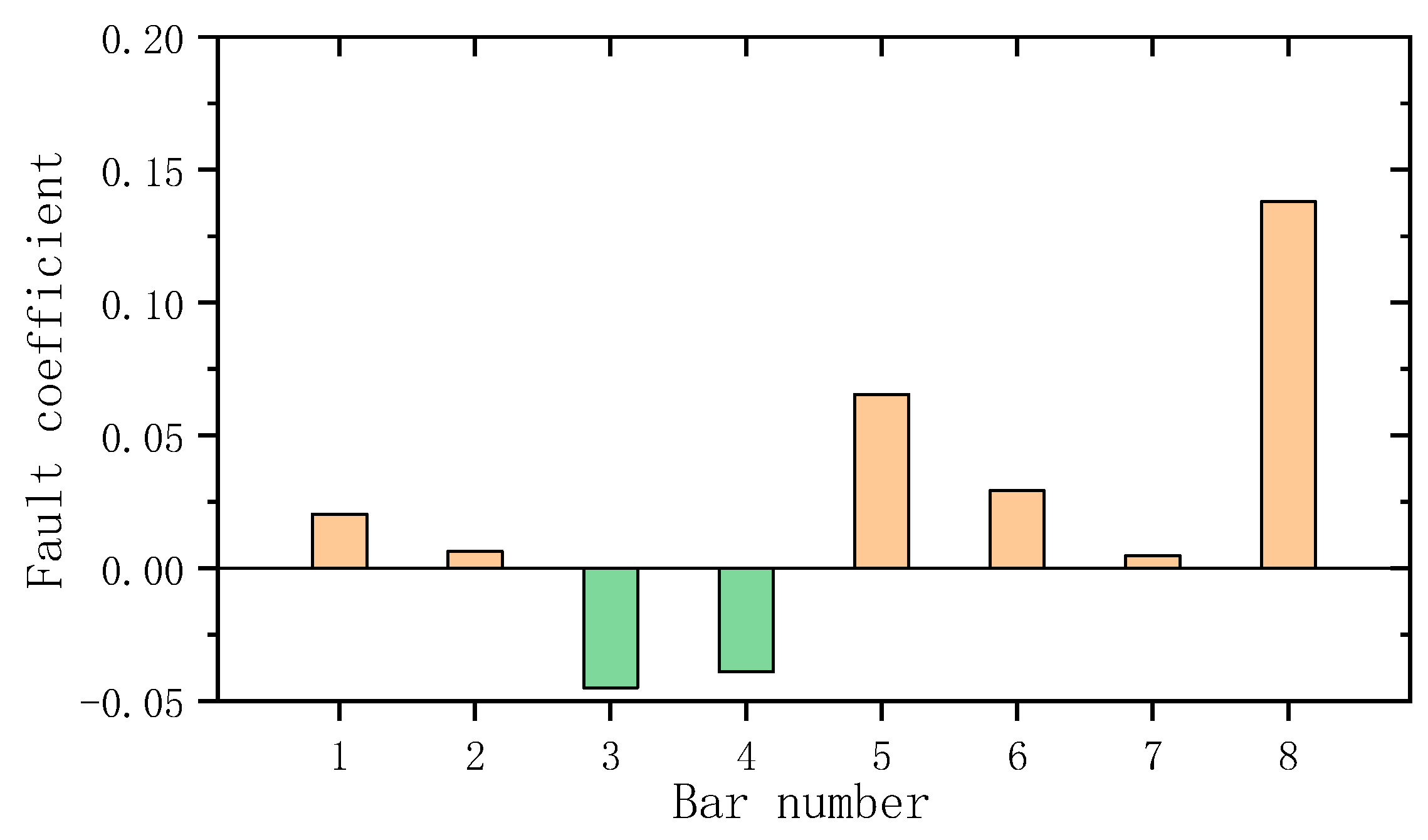
4. Experimental Verification

As presented in Figure 13a, the proposed hybrid sensitivity method was further verified using an experimental steel beam with fixed ends. Obviously, this beam structure could basically be regarded as a geometrically symmetric structure. The main physical parameters of the structure were as follows: the elastic modulus was 193 GPa, the density was 7850 kg/m³, the length of the beam was 0.8 m, and the width and height of the cross-section were 15 mm and 3 mm, respectively. The geometric parameters of the beam and the arrangement of measurement points are shown in Figure 13b. In the static test, the vertical displacements of nodes 3–5 were observed through the dial indicators. The reason for selecting these static measurement points was that they were all located in the mid-span area, and the corresponding vertical displacements under the given gravity load were relatively large and easy to measure. In the dynamic test, the accelerometers were arranged in the vertical direction of nodes 1, 2, 6, and 7 to extract the first-order vibration mode using the vibration test system. The purpose of selecting these dynamic measurement points was to monitor the entire structure as they were located in the areas not measured during the static testing.

As stated before, the asymmetric gravity loading could overcome the possible missed diagnosis problem in the defect diagnosis of the symmetrical structure. For this purpose, the gravity loading, as shown in Figure 14, applied a concentrated force of 10 N at node 3 of the structure, i.e., the location that was a distance of 300 mm from the left end. As a by-product of static loading, the gravity load and the structure were connected using strong adhesive to form a new added-mass system. Both the original structure and the added-mass structure underwent dynamic testing to obtain the first-order vibration modal data, as shown in Figure 15. Figure 16 shows the damaged beam with a notch. As shown in Figure 16, the cut width (approximately 3 + 3 = 6 mm) accounted for 40% of the entire cross-sectional width of 15 mm. For the fault diagnosis, the undamaged FEM with eight elements, as shown in Figure 17 for the beam, was established using MATLAB software of 7.0 version to represent the undamaged beam. Note that the number in the circle in Figure 17 denotes the element number in the FEM. Obviously, the damage location was related to the fifth element in this FEM with eight elements, as shown in Figure 17. Figure 18, Figure 19 and Figure 20 present the calculation results of the fault coefficients using a pure static algorithm, a pure dynamic algorithm, and the proposed hybrid method, respectively. From Figure 18, Figure 19 and Figure 20, one can find that the fault coefficients obtained using the hybrid method more clearly indicated that the fault was located in element 5. Specifically, the fault coefficients of element 5 obtained using the pure static method, the pure dynamic method, and the hybrid method were 6.55%, 13.6%, and 24.1%, respectively.

Next, a more refined FEM with sixteen elements, as shown in Figure 21, was established to discuss the impact of FEM mesh density on the damage diagnosis results. Note that the number in the circle in Figure 21 denotes the element number in the refined FEM. Obviously, the damage location was related to the tenth element in this refined FEM with sixteen elements, as shown in Figure 22. Compared with the FEM of eight elements, the number of unknown fault coefficients in the FEM with sixteen elements that needed to be solved had doubled from 8 to 16. Based on this refined FEM, Figure 23, Figure 24 and Figure 25 present the calculation results of the fault coefficients using a pure static algorithm, a pure dynamic algorithm, and the proposed hybrid method, respectively. One can find that the fault coefficients obtained using the hybrid method more clearly indicated that the fault was located in element 10. Specifically, the fault coefficients of element 10 obtained using the pure static method, the pure dynamic method, and the hybrid method were 7.7%, 9.3%, and 33.2%, respectively. Obviously, the calculated fault coefficient (33.2%) obtained using the hybrid method was the closest to the true value (approximately 40%). It showed that the diagnosis result of the proposed method was the most reliable and accurate. The above results indicated that a more refined FEM would contribute to a more accurate damage localization result. However, the meshing of the FEM was not necessarily as dense as possible since an FEM with more elements clearly increased the number of unknown fault coefficients. This meant that an FEM with more elements may have required more test data to successfully compute the fault coefficients for the damage identification. It should also be noted that the damage extents calculated by these two FEMs were different because the lengths of the elements changed. As shown in Figure 22, the fault coefficient corresponding to the same notch changed for the different element grids. The fault coefficients calculated by an FEM with sparse grid partitioning are usually smaller than those obtained by an FEM with dense grid partitioning.

5. Conclusions

In this article, a hybrid sensitivity method was developed by combining the static displacement and the dynamic mode shape to find a fault’s location and extent in a structure. The greatest innovation of the proposed method was its use of static loading as a new added-mass system to obtain more vibration parameters for defect diagnosis. The proposed method can avoid the shortcoming of the possible missed diagnosis, which is seen when using pure static and pure dynamic methods, and it obtained more reliable and accurate fault diagnosis results. A steel roof truss structure with 25 bar elements was used as a numerical example to illustrate the feasibility and advantages of the proposed method. An experimental steel beam was further used to verify the proposed method. By comparing the pure static algorithm, the pure dynamic algorithm, and the hybrid algorithm, the following main conclusions could be obtained: (1) The symmetry of a structure may lead to a missed diagnosis when using pure static or pure dynamic methods. The adverse effect of structural symmetry on defect diagnosis can be overcome by using asymmetric gravity loading. Among the three methods, the diagnosis result of the proposed hybrid method was the most reliable and accurate. (2) For a single defect condition, the three methods may be able to indicate the location of the defect, but the accuracy of the damage extent obtained by the proposed method was the highest. (3) For multiple defect conditions, only the proposed hybrid method could accurately indicate the locations of all the defects while the pure static method and the pure dynamic method missed diagnoses. The proposed method can provide a reference for structural defect diagnosis in engineering practice, especially for symmetric structures. We note that this work mainly elaborated on the application of this hybrid method in diagnosing structural on-site faults. The proposed method may also be used for desk research during design, and further research in this area can be carried out in the future.

References

1. Sun, Y.; Yang, Q.; Peng, X. Damage Identification for Shear-Type Structures Using the Change of Generalized Shear Energy. Coatings 2022, 12, 192. [Google Scholar] [CrossRef]
2. Sun, Y.; Yang, Q.; Peng, X. Structural Damage Assessment Using Multiple-Stage Dynamic Flexibility Analysis. Aerospace 2022, 9, 295. [Google Scholar] [CrossRef]
3. Fang, R.; Wu, Y.; Wei, W.; Na, L.; Biao, Q.; Jiang, P.; Yang, Q. An Improved Static Residual Force Algorithm and Its Application in Cable Damage Identification for Cable-Stayed Bridges. Appl. Sci. 2022, 12, 2945. [Google Scholar] [CrossRef]
4. Yang, Q.; Sun, B. Structural damage localization and quantification using static test data. Struct. Health Monit. 2010, 10, 381–389. [Google Scholar] [CrossRef]
5. Yang, Q.W. Fast and Exact Algorithm for Structural Static Reanalysis Based on Flexibility Disassembly Perturbation. AIAA J. 2019, 57, 3599–3607. [Google Scholar] [CrossRef]
6. Yang, Q.; Peng, X. A Fast Calculation Method for Sensitivity Analysis Using Matrix Decomposition Technique. Axioms 2023, 12, 179. [Google Scholar] [CrossRef]
7. Yang, Q.; Wang, C.; Li, N.; Luo, S.; Wang, W. Model-Free Method for Damage Localization of Grid Structure. Appl. Sci. 2019, 9, 3252. [Google Scholar] [CrossRef]
8. Bakhtiari-Nejad, F.; Rahai, A.; Esfandiari, A. A structural damage detection method using static noisy data. Eng. Struct. 2005, 27, 1784–1793. [Google Scholar] [CrossRef]
9. Abdo, M.A.B. Parametric study of using only static response in structural damage detection. Eng. Struct. 2012, 34, 124–131. [Google Scholar] [CrossRef]
10. Tian, S.; Yang, Z.; Chen, X.; Xie, Y. Damage Detection Based on Static Strain Responses Using FBG in a Wind Turbine Blade. Sensors 2015, 15, 19992–20005. [Google Scholar] [CrossRef]
11. Santos, J.; Cremona, C.; Orcesi, A.; Silveira, P.; Calado, L. Static-based early-damage detection using symbolic data analysis and unsupervised learning methods. Front. Struct. Civ. Eng. 2015, 9, 1–16. [Google Scholar] [CrossRef]
12. Viola, E.; Bocchini, P. Non-destructive parametric system identification and damage detection in truss structures by static tests. Struct. Infrastruct. Eng. 2013, 9, 384–402. [Google Scholar] [CrossRef]
13. Terlaje, A.S., III; Truman, K.Z. Parameter identification and damage detection using structural optimization and static response data. Adv. Struct. Eng. 2007, 10, 607–621. [Google Scholar] [CrossRef]
14. Boumechra, N. Damage detection in beam and truss structures by the inverse analysis of the static response due to moving loads. Struct. Control. Health Monit. 2016, 24, e1972. [Google Scholar] [CrossRef]
15. Peng, X.; Yang, Q. Damage detection in beam-like structures using static shear energy redistribution. Front. Struct. Civ. Eng. 2022, 16, 1552–1564. [Google Scholar] [CrossRef]
16. Chrysanidis, T. Experimental and numerical research on cracking characteristics of medium-reinforced prisms under variable uniaxial degrees of elongation. Eng. Fail. Anal. 2023, 145, 107014. [Google Scholar] [CrossRef]
17. Lu, Z.; Law, S. Features of dynamic response sensitivity and its application in damage detection. J. Sound Vib. 2007, 303, 305–329. [Google Scholar] [CrossRef]
18. Feng, D.; Feng, M.Q. Computer vision for SHM of civil infrastructure: From dynamic response measurement to damage detection—A review. Eng. Struct. 2018, 156, 105–117. [Google Scholar] [CrossRef]
19. Gentile, C.; Guidobaldi, M.; Saisi, A. One-year dynamic monitoring of a historic tower: Damage detection under changing environment. Meccanica 2016, 51, 2873–2889. [Google Scholar] [CrossRef]
20. Cardoso, R.D.A.; Cury, A.; Barbosa, F. Automated real-time damage detection strategy using raw dynamic measurements. Eng. Struct. 2019, 196, 109364. [Google Scholar] [CrossRef]
21. Yang, Q.W.; Peng, X. A highly efficient method for structural model reduction. Int. J. Numer. Methods Eng. 2022, 124, 513–533. [Google Scholar] [CrossRef]
22. Yang, Q.; Peng, X. Sensitivity Analysis Using a Reduced Finite Element Model for Structural Damage Identification. Materials 2021, 14, 5514. [Google Scholar] [CrossRef] [PubMed]
23. Peng, X.; Yang, Q.-W. Sensor Placement and Structural Damage Evaluation by Improved Generalized Flexibility. IEEE Sensors J. 2021, 21, 11654–11664. [Google Scholar] [CrossRef]
24. Weng, S.; Zhu, H.; Xia, Y.; Li, J.; Tian, W. A review on dynamic substructuring methods for model updating and damage detection of large-scale structures. Adv. Struct. Eng. 2019, 23, 584–600. [Google Scholar] [CrossRef]
25. Meixedo, A.; Santos, J.; Ribeiro, D.; Calçada, R.; Todd, M. Damage detection in railway bridges using traffic-induced dynamic responses. Eng. Struct. 2021, 238, 112189. [Google Scholar] [CrossRef]
26. Yang, Q.; Peng, X. An Exact Method for Calculating the Eigenvector Sensitivities. Appl. Sci. 2020, 10, 2577. [Google Scholar] [CrossRef]
27. Yang, Q.; Sun, B.; Lu, C. An improved spectral decomposition flexibility perturbation method for finite element model updating. Adv. Mech. Eng. 2018, 10, 1687814018814920. [Google Scholar] [CrossRef]
Figure 1. Flowchart of the entire technique.
Coatings 13 00920 g001
Figure 2. A steel roof structure.
Coatings 13 00920 g002
Figure 3. Layout of the loading and the measuring points.
Coatings 13 00920 g003
Figure 4. Fault coefficients obtained using a pure static algorithm (bar 3 is damaged).
Coatings 13 00920 g004
Figure 5. Fault coefficients obtained using a pure dynamic algorithm (bar 3 is damaged).
Coatings 13 00920 g005
Figure 6. Fault coefficients obtained using the proposed hybrid algorithm (bar 3 is damaged).
Coatings 13 00920 g006
Figure 7. Fault coefficients obtained using a pure static algorithm (bar 8 is damaged).
Coatings 13 00920 g007
Figure 8. Fault coefficients obtained using a pure dynamic algorithm (bar 8 is damaged).
Coatings 13 00920 g008
Figure 9. Fault coefficients obtained using the proposed hybrid algorithm (bar 8 is damaged).
Coatings 13 00920 g009
Figure 10. Fault coefficients obtained using a pure static algorithm (bars 12 and 20 are damaged).
Coatings 13 00920 g010
Figure 11. Fault coefficients obtained using a pure dynamic algorithm (bars 12 and 20 are damaged).
Coatings 13 00920 g011
Figure 12. Fault coefficients obtained using the proposed hybrid algorithm (bars 12 and 20 are damaged).
Coatings 13 00920 g012
Figure 13. (a) An experimental steel beam with fixed ends. (b) Geometric parameters and measurement locations (unit: mm).
Coatings 13 00920 g013
Figure 14. Static testing.
Coatings 13 00920 g014
Figure 15. (a) Dynamic testing for the original system. (b) Dynamic testing for the added-mass system.
Coatings 13 00920 g015
Figure 16. (a) The damaged beam with a notch. (b) Size of the notch (unit: mm).
Coatings 13 00920 g016
Figure 17. FEM with eight elements (unit: mm).
Coatings 13 00920 g017
Figure 18. Fault coefficients of the FEM with eight elements obtained using the pure static algorithm (element 5 is damaged).
Coatings 13 00920 g018
Figure 19. Fault coefficients of the FEM with eight elements obtained using the pure dynamic algorithm (element 5 is damaged).
Coatings 13 00920 g019
Figure 20. Fault coefficients of the FEM with eight elements obtained using the proposed hybrid algorithm (element 5 is damaged).
Coatings 13 00920 g020
Figure 21. A refined FEM with sixteen elements (unit: mm).
Coatings 13 00920 g021
Figure 22. Defect location and the corresponding element number in different FEMs (the number in the circle denotes the element number in the FEM).
Coatings 13 00920 g022
Figure 23. Fault coefficients of the FEM with sixteen elements obtained using the pure static algorithm (element 10 is damaged).
Coatings 13 00920 g023
Figure 24. Fault coefficients of the FEM with sixteen elements obtained using the pure dynamic algorithm (element 10 is damaged).
Coatings 13 00920 g024
Figure 25. Fault coefficients of the FEM with sixteen elements obtained using the proposed hybrid algorithm (element 10 is damaged).
Coatings 13 00920 g025
Disclaimer/Publisher’s Note: The statements, opinions and data contained in all publications are solely those of the individual author(s) and contributor(s) and not of MDPI and/or the editor(s). MDPI and/or the editor(s) disclaim responsibility for any injury to people or property resulting from any ideas, methods, instructions or products referred to in the content.