Residual Stress Relaxation in the Laser Welded Structure after Low-Cycle Fatigue and Fatigue Life: Numerical Analysis and Neutron Diffraction Experiment

Abstract

The residual stress relaxation behaviour in low-cycle fatigue brings uncertainty to accurately predict fatigue life. Therefore, establishing the residual stress relaxation model for the welded structure is critical. In this paper, the residual stress is simulated through Abaqus finite element software (6.14). The residual stress relaxation model related to the magnitude of cyclic loading and the number of cycles is proposed. Furthermore, the residual stress relaxation model is applied to predict low-cycle fatigue life. Finally, the simulation results are validated by experimental data obtained using the reliable neutron diffraction method, and a good agreement is observed.

1. Introduction

Laser welding (LW) has developed considerably, in terms of improving efficiency and reducing costs, in the past decade because of its advantages that include rapid welding speed, small heat-affected zone, and low residual stress (RS) [1]. It has gradually taken the place of conventional welding techniques, such as inert tungsten gas (TIG), inert metal gas (MIG), and electron beam welding [2]. The characteristics of LW and other welding methods are shown in

Table 1. Characteristics of LW and other welding methods [3,4,5].

Welding Method	Welding Speed	Penetration	Advantages	Disadvantages
Laser beam	1–5 m/min	Up to 10 mm	High welding speedLess deformation	High initial costs Limited material compatibility
TIG	0.1–0.5 m/min	3–4 mm	High quality	High equipment costs
MIG	0.5–1 m/min	3–4 mm	Low costs	Large deformation Limited welding positions
Electron beam	1–10 m/min	Up to 80 mm	High welding speed	Vacuum required Limited penetration depth

.

LW can be seen as a process in which the energy-carrying laser beam interacts with the material. The material absorbs a part of the energy and reflects the rest. The deep penetration welding process is complex, with a dynamic molten pool and keyhole, accompanied by intense chemical and physical reactions, including laser-induced plasma, keyhole formation, fluid dynamics of the molten pool, metal melting and solidification, etc. The deep penetration welding process can be divided into a preheating period, a molten pool formation period, and a keyhole formation period. In the preheating period, the laser preheats the surface of the material, and the reflection of the laser beam dominates the process. In the molten pool formation period, the material is rapidly heated up to the melting point as the temperature rises, increasing the material’s absorption rate (of the laser). In the keyhole formation period, the temperature reaches the boiling point, and intense vaporization takes place. The interaction of recoil pressure which is brought on by vaporization, Marangoni force, liquid gravity, and buoyancy, results in the appearance of the keyhole. The existence of the keyhole further improves the capacity of the material to absorb the laser beam energy [6]. The deep penetration welding process is shown in Figure 1.

Due to the thermal effects of the LW process, the RS inevitably presents in the welded structure [7]. RS can be divided into three types. Type one: macro RS, which develops in the structure on a scale larger than the grain size. Type two: micros RS, which varies with the scale of a single grain. Type three: micro RS, which exists within a single grain, mainly due to dislocations and other crystallographic defects [8]. In this paper, the analysis focuses on the first type of RS.

Generally, the engineering structure is designed so that the material only deforms in an elastic manner [9]. However, the welded structure widely used in various engineering applications is inevitably subjected to monotonic, cyclic, or random fluctuating loading during service [10]. Although the maximum stress induced by the dynamic loading is lower than the yield strength (σ_y), local plastic deformation may result from the superposition of the complex stress state and the RS of LW, which can affect the fatigue behaviour [11]. The combination can even alter the location of fatigue failure, unexpectedly causing the damage behaviour. Fatigue failure usually results in considerable expenditure to repair and restore equipment and structure [8]. Therefore, a comprehensive review of the distribution and variation of RS, both before and after the fatigue process, is essential to accurately calculate the fatigue life (N_f) of the welded structure.

It is well known that N_f can be improved by reducing and eliminating RS. Researchers have developed N_f prediction models that take into account the effects of RS. Nevertheless, most of these methods consider RS as the mean stress (σ_m) or the constant [12]. However, cyclic loading causes stress reversal and accumulation of plastic strain [13], which results in the decrease of a part or total RS, this behaviour is known as “RS relaxation”. Estimates of N_f that do not take RS relaxation into account can lead to imprecise results [14]. The pattern of RS relaxation varies depending on the process condition, loading type, and material. The phenomenon of RS relaxation can be classified as quasi-static, cyclic, and crack-induced relaxation. Quasi-static relaxation results from macroscopic yielding that occurs within the initial cycles when the combination of cyclic loading and the RS of LW is higher than σ_y, and the relaxation is usually the most significant. Cyclic relaxation, related to the movement of dislocations, is the relaxation resulting from microscopic plastic deformation during cyclic loading, even though the summed stress is lower than σ_y. Crack relaxation occurs at the final stage of cyclic loading and is activated by the initiation and propagation of the crack. In order to incorporate the effects of RS into fatigue life evaluation methods more completely, it is necessary to develop an effective method or model that can predict RS relaxation behaviour accurately [15].

Many empirical methods are used to describe RS relaxation including, for example, linear logarithmic, exponential, or power functions. Morrow and Sinclair proposed replacing RS relaxation with σ_m relaxation, and established the relationship between σ_m relaxation and the number of cycles as follows [16]:

$$\frac{{\sigma }_{m\mathrm{N}}}{{\sigma }_{m1}}=\frac{{\sigma }_y-{\sigma }_a}{{\sigma }_{m1}}-{\left(\frac{{\sigma }_a}{{\sigma }_y}\right)}^b\log N$$

(1)

where σ_mN is the σ_m after N cycles, σ_m1 is the σ_m after the first cycle, σ_a is cyclic loading, b is the material constant, N is the cycle numbers. Jhansale and Topper similarly suggest describing σ_m relaxation as a function of the number of cycles, as follows [17]:

$${\sigma }_{\mathrm{mN}}={\sigma }_{m1}{(N)}^B$$

(2)

where B is the relaxation exponent of material. Unfortunately, the above two models only apply when the stress ratio is −1. Kodama proposed a relationship between RS relaxation and the number of cycles [18].

$${\sigma }_{\mathrm{N}}^{re}=A+m\log N$$

(3)

where ${\sigma }_{\mathrm{N}}^{re}$ is the RS after N cycles, and A and m are material constants. However, it is worth noting that this model can only support the RS relaxation behavior after the first cycle. Holzapfe proposed that RS relaxation occurs because of micro-plastic strain accumulating, and suggested that RS relaxation can be calculated as follows [19]:

$${\sigma }_{rs}={\sigma }_{rs}(N-1)-\mu \log N$$

(4)

where σ_rs(N – 1) is the RS after the first cycle, and μ is the material constant.

The above equations make it clear that the empirical models only consider the effects of the number of cycles on RS relaxation. Nevertheless, there are many influencing parameters for RS relaxation, such as the magnitude of the initial RS, loading type, and loading amplitude [20]. Despite the fact that researchers have carried out a great deal of research in this area, much work still needs to be done [21].

Previous research [22] presented the plastic constitutive models for strain hardening, temperature softening, and strain rate hardening, briefly explaining that RS relaxes and redistributes in the heat-affected zone and welds after low-cycle fatigue (LCF). This paper extends this previous work to analyze the factors affecting RS relaxation, and proposes the RS relaxation model that considers the magnitude of cyclic loading (C_M) and the number of cycles (C_N). Meanwhile, the RS relaxation model is applied to predict the N_f of LCF. The appropriateness of these models is verified by the results of LCF and neutron diffraction (ND) experiments. First, the sequential coupled thermo-mechanical finite element (FE) model is created by Abaqus, including the heat source model and several plastic constitutive models, to simulate the RS of LW. The determined RS of LW is incorporated into the subsequent step of the simulation, as the initial RS, and the RS of LCF is calculated by using the direct cyclic method and combined hardening model. The RS relaxation model is then proposed by comparing the relaxation behaviour of different C_M and C_N, and compared to available ND experimental results. Finally, LCF life is predicted by the modified N_f model with considering the RS relaxation behaviour. The numerical and experimental results show a good degree of agreement.

2. Materials and Methods

In this paper, DP600 steel is selected as the base metal, with dimensions of 180 mm × 170 mm × 1.25 mm.

Table 2. The main chemical compositions of DP600 in weight percentage [2].

C	Mn	P	S	Al	Cr	Si	Ni	Fe
0.10	1.09	0.03	0.001	1.19	0.02	0.26	0.01	97.20

presents the main chemical compositions for DP600 at room temperature (25 °C). Dual-phase (DP) steel is part of advanced high-strength steel and is usually produced by annealing and then rapid cooling. Microstructures consisting of a ferrite matrix and dispersed martensite islands are produced by the well-controlled thermo-mechanical process. Strength can be increased by adequately regulating the content, morphology, and distribution of martensite, while ductility can also be achieved, which meets the needs of engineering applications [23]. DP steel exhibits lower σ_y (370 ± 40 Mpa), but the continuous yield behaviour contributes to larger elongation (23 ± 1%) and higher tensile strength (654 ± 14 Mpa) [24]. The continuous yielding behaviour of DP steel occurs because of the formation of austenite in the ferrite matrix during annealing, followed by the conversion of austenite to martensite during rapid cooling [2]. A hard phase is therefore introduced into the microstructure that resists deformation during the transformation from austenite to martensite. The volume expansion leads to the formation of mobile dislocation in the ferrite matrix. The dislocation movement and their interaction leads to continuous yielding behaviour, giving DP steel a high initial strain hardening rate and the ability to accommodate the majority of the plastic deformation [25].

3. Experiments and Tests

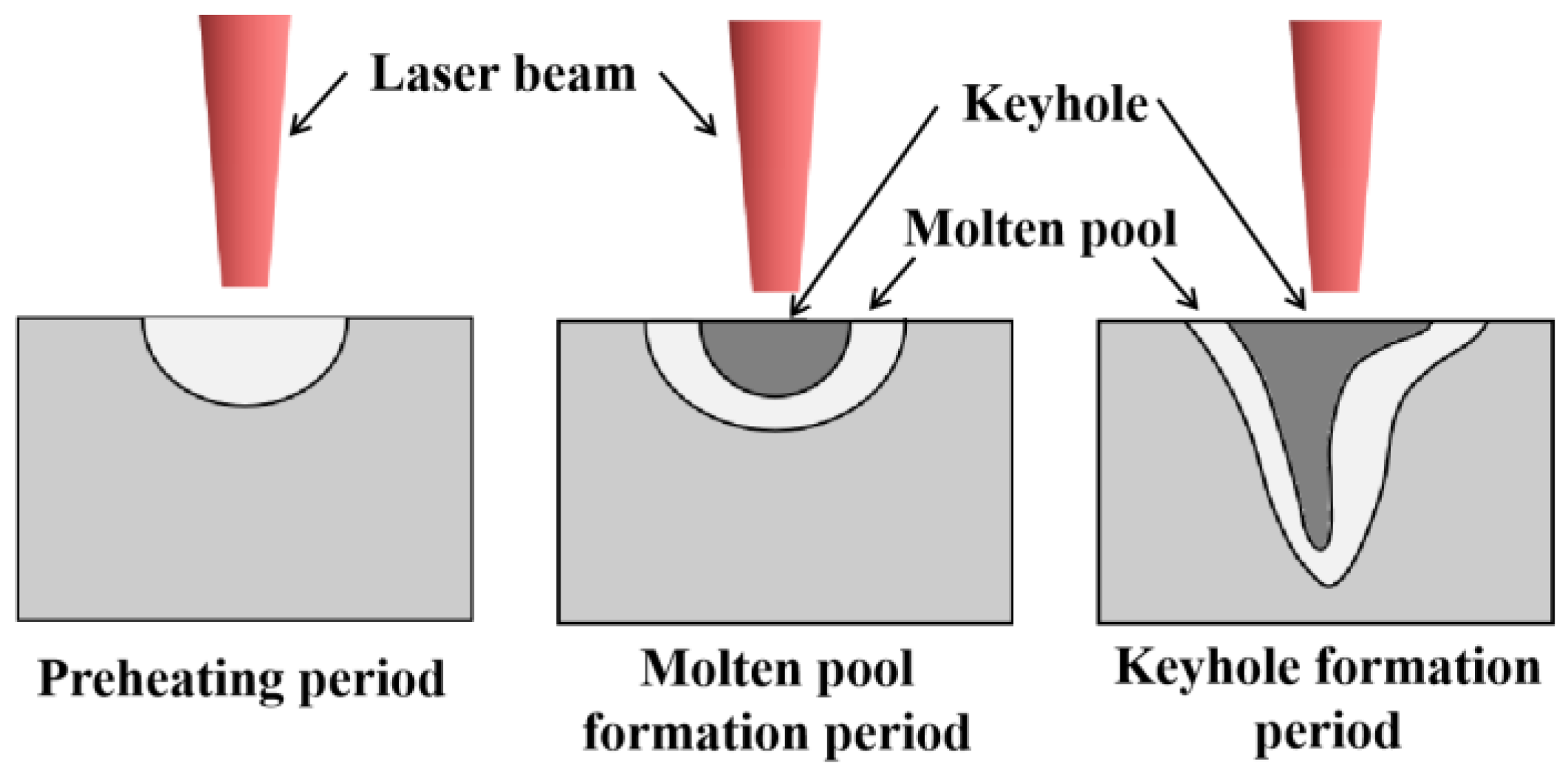
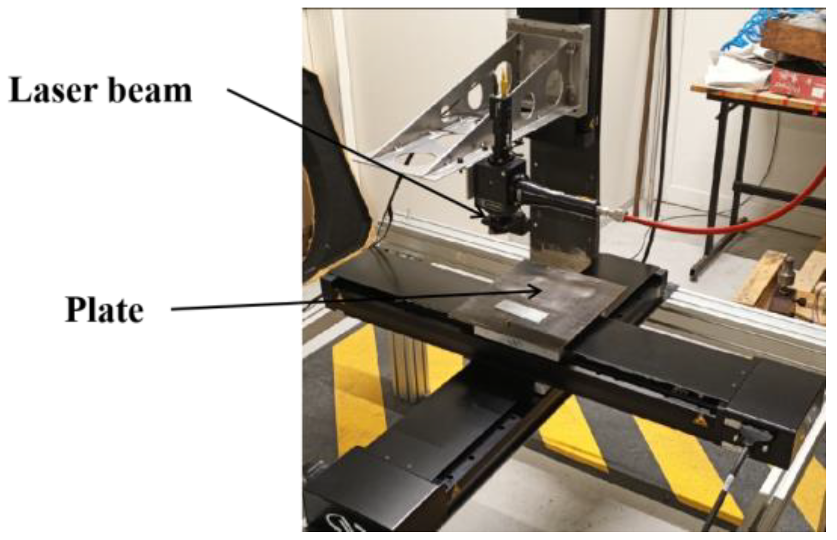
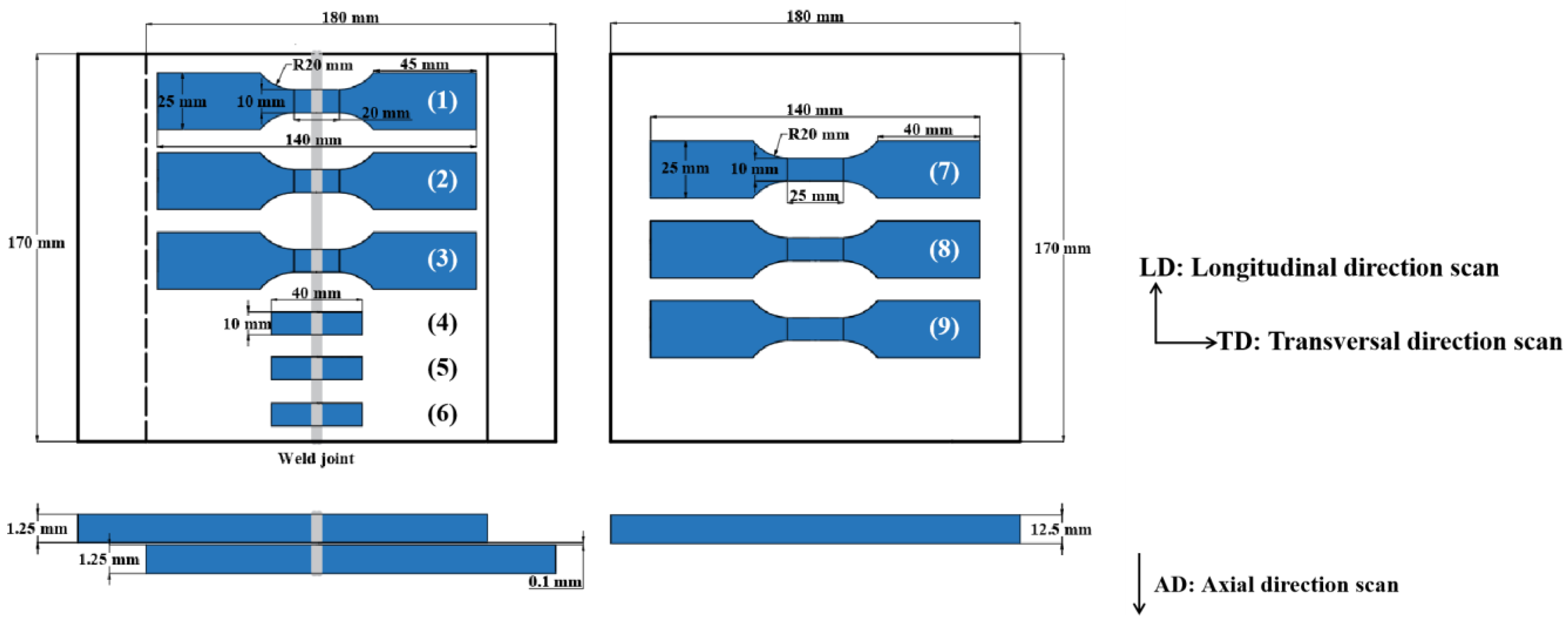
3.1. Laser Welding Experiment

The LW process is performed using the neodymium-yttrium aluminium garnet (Nd: YAG) continuous laser equipment, comprising a 4 Kw generator and a Fanuc R2000Ib arm robot. Nd: YAG solid-state laser is one of the most commonly used lasers in the industry, which consists of neodymium element dispersed in the host yttrium aluminum garnet (YAG) crystal. The Nd: YAG crystal causes photons to be released in random spatial directions through a combination of spontaneous and excited emission mechanisms. The photons return to the crystal by striking the reflecting and transmitting mirrors, and continue to stimulate the emission of other photons. This activity greatly amplifies the photons moving back and forth between the mirrors, constantly stimulating and redirecting their direction of travel and finally guiding them to the target with the help of turning mirrors and focusing optics. The platform of the Nd: YAG laser is shown in Figure 2. The process parameters include a laser power of 3500 W, a welding speed of 3 m/min, and a thermal efficiency of 42%. Argon has a flow rate of 20 cubic feet per hour and is employed as the shielding gas.

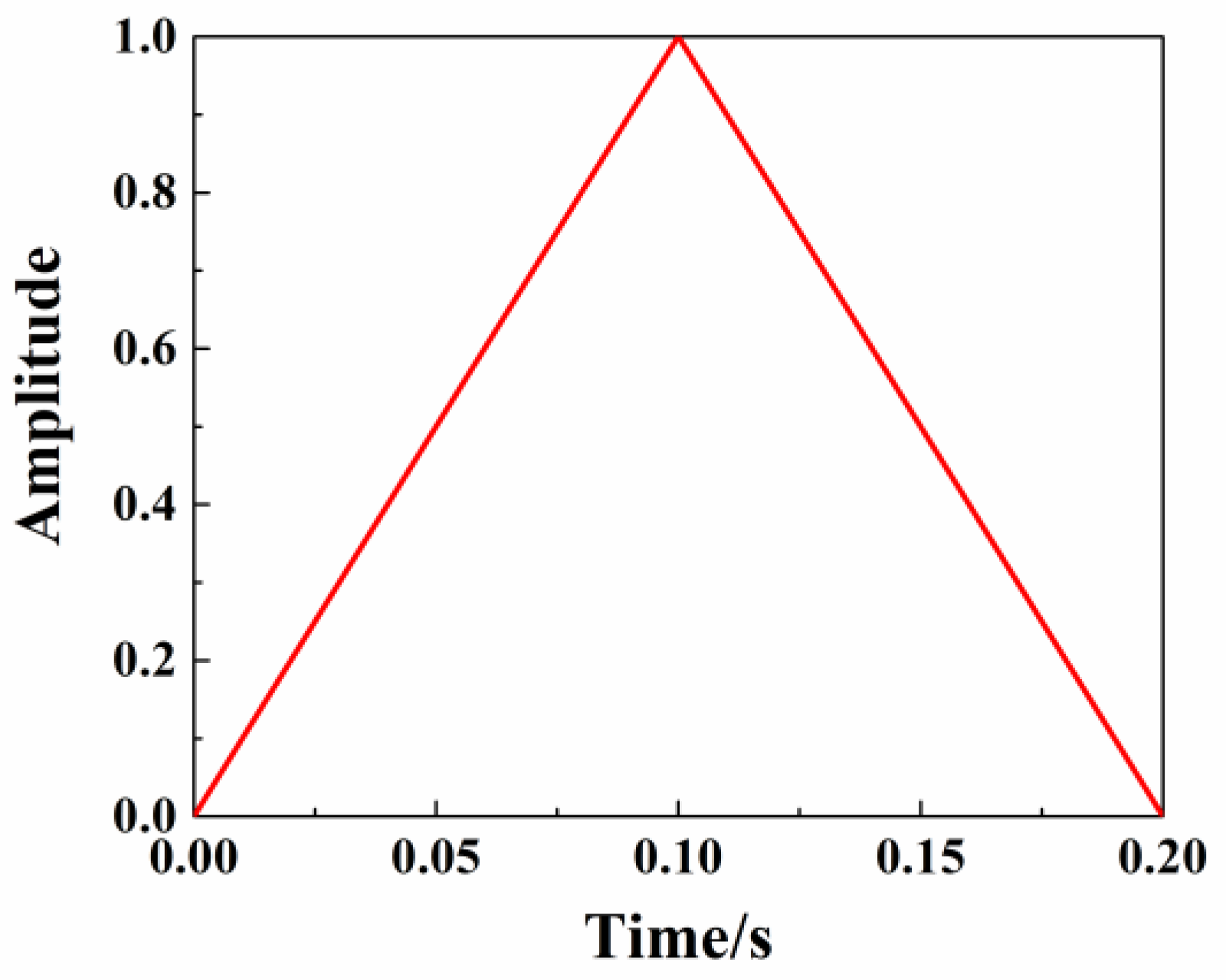
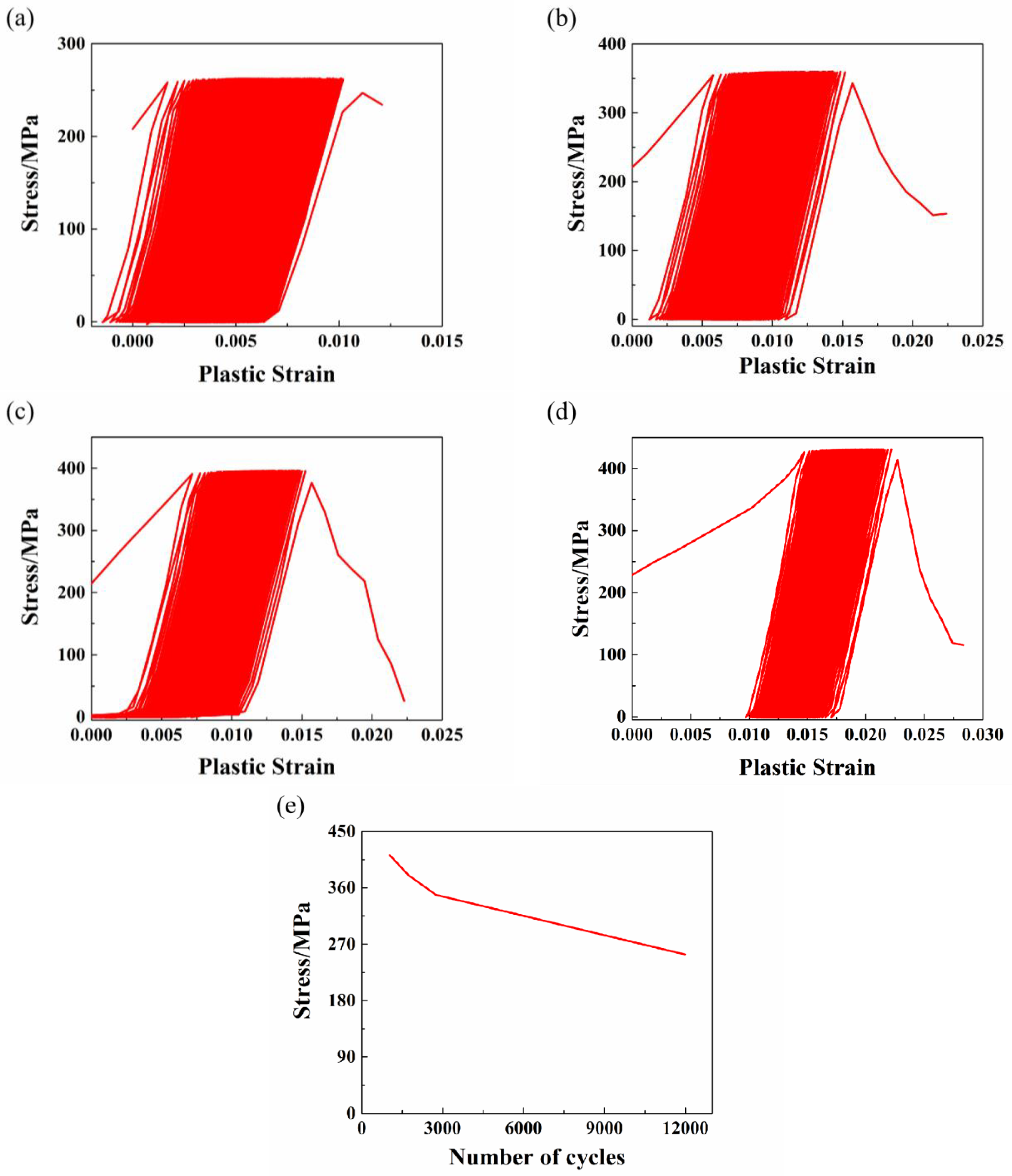
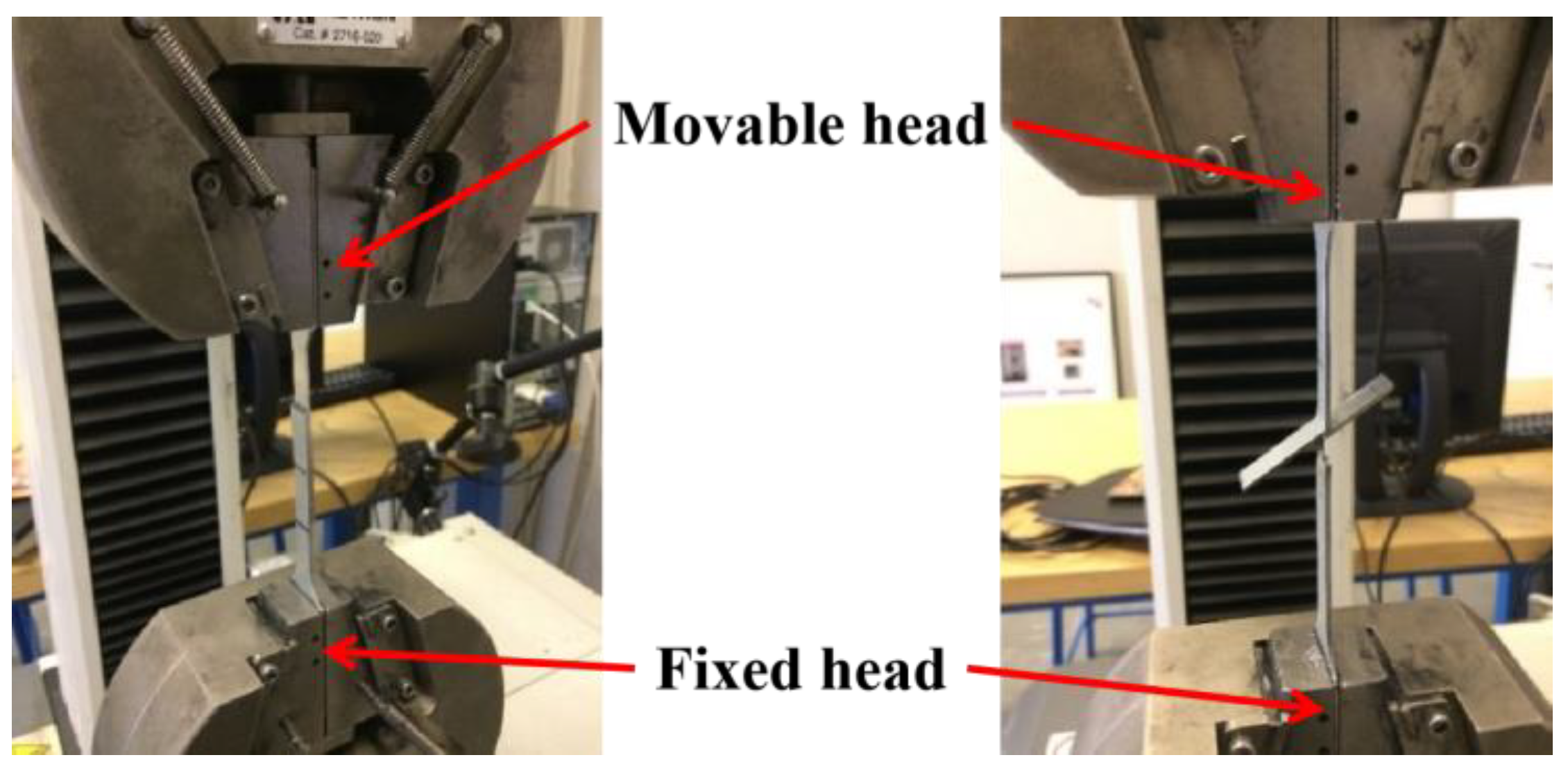
3.2. Low-Cycle Fatigue Experiment

The Instron 3369 LCF experimental machine controlled by Instron software is employed to conduct the cyclic behaviour of the laser welded structure. The LCF experimental specimens are fabricated according to ASTM E606 [26]. Figure 3 shows the corresponding geometry and dimensions. The overlap area thickness is 2.6 mm, and the lap joint gap is 0.1 mm. The experiment is carried out at room temperature with a maximum stress of 250, 300, 380, and 400 Mpa, a stress ratio of 0, and a triangular waveform for the applied stress (Figure 4). During the experiment, all the cyclic data are recorded and analyzed by the Bluehill 3 software, including displacement force as a function of the time, and C_N until failure. These parameters are monitored to construct the cyclic σ-ε curve and N_f curve (Figure 5). The platform and specimens, both before and after the LCF experiment, are shown in Figure 6.

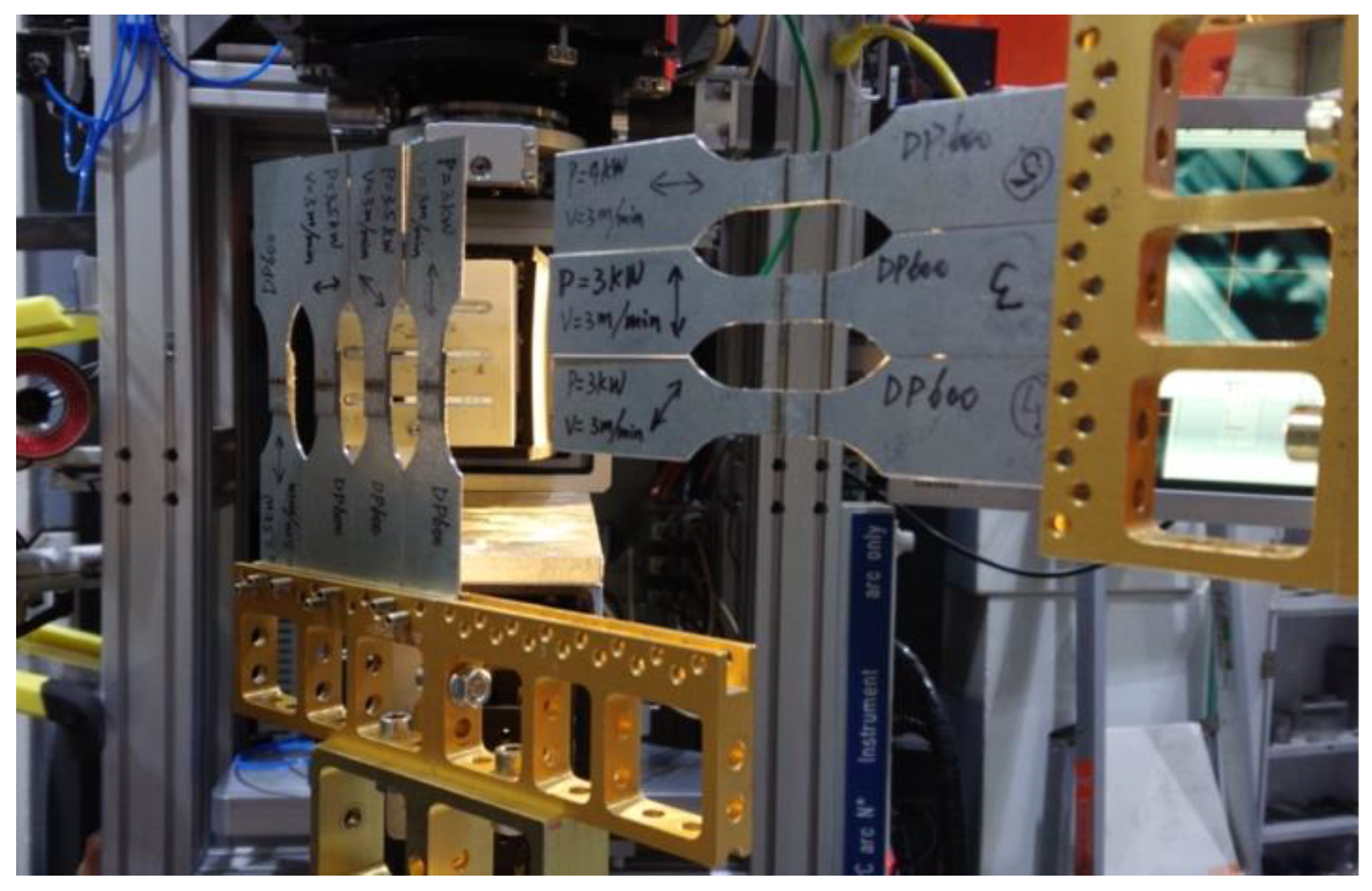
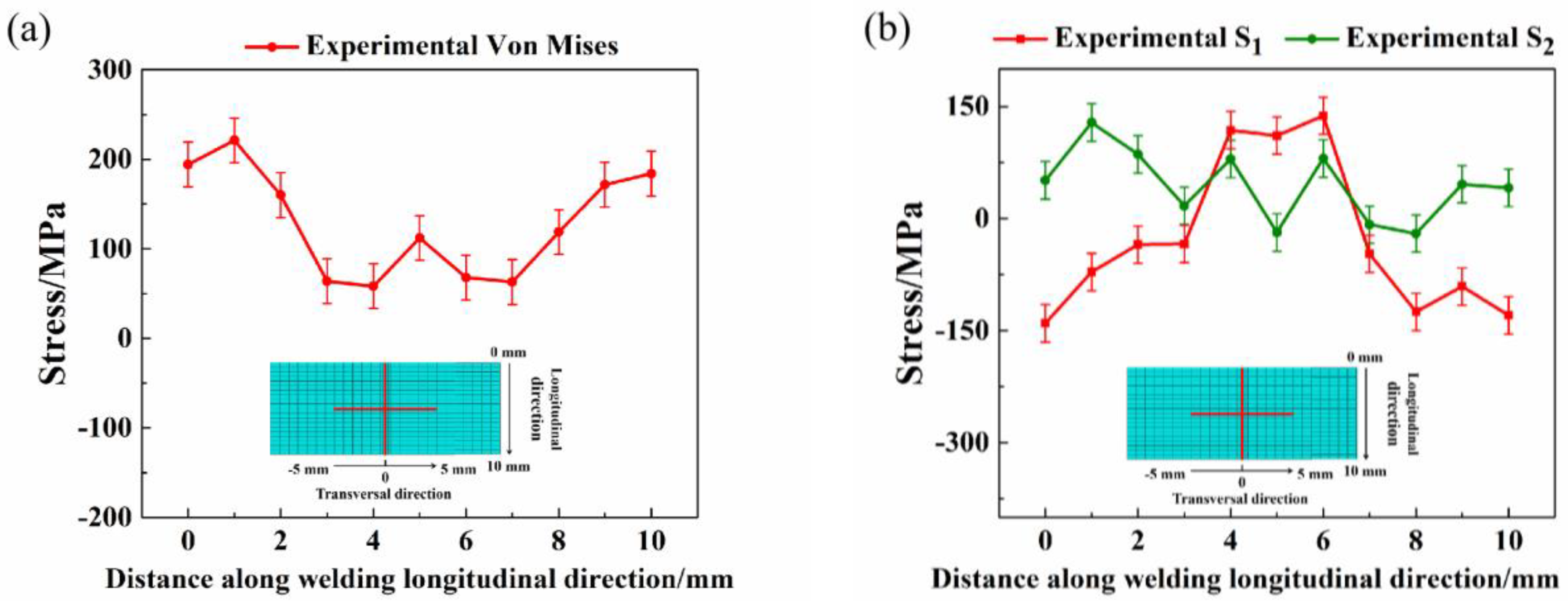
3.3. Neutron Diffraction Experiment

The reliable RS measurement method is very important [27], and diffraction is the most widely used and mature method of non-destructive testing, including X-ray diffraction, ND, and X-ray synchrotron radiation [28]. In this paper, ND is used to measure the RS of LW and LCF, and Figure 7 shows the schematic of the ND experiment. The RS of LW is measured after the welded structure has completely cooled. The RS of LCF is measured when the fatigue experiment is stopped at predefined cycles. The measurement path has been pre-marked on the specimens, and the position is the same for each measurement [29]. Three repeated ND experiments are performed to ensure the results are correct. In Figure 3, specimens 1 to 3 are used to measure the RS of LCF of the welded structure; specimens 4 to 6 are used to measure the RS of LW of the welded structure; and specimens 7 to 9 are used to measure the RS of LCF of the base metal.

The ND experiment is performed on the dedicated SALSA diffractometer at the Institute Laue Langevin (ILL) in Grenoble. Two adjacent measurement points are placed 1 mm apart, and each measurement point has a gauge volume of 0.6 mm × 0.6 mm × 1 mm. The strain at each measurement point is measured in three orthogonal directions, which is achieved by mounting each sample in three different directions [8]. The neutron wavelength is set to 0.287 nm, the value of diffraction angle 2θ for {211} reflection is equal to 93.45°, and the unstressed lattice spacing is measured on the DP600, with d₀ of 1.704 Å [30]. Young’s modulus (E) and Poisson’s ratio (v) are obtained by the self-consistent elastic calculation. The results show that E is between 230 and 236 Gpa and v is between 0.27 and 0.30. These values show that the elastic anisotropy remains very low. Therefore, the elastic isotropic Hooke’s law (Equation (5)) is used to calculate the triaxial RS on the basis of the measured strain values [28]. Figure 8 shows the experimental results of the RS of LCF (Von Mises) and principal stress curves along the longitudinal direction. S₁ and S₂ correspond to the principal stress in the x-direction and y-direction.

$${\sigma }_i=\frac{E_{211}}{1+{\nu }_{211}}\left[{\epsilon }_i+\frac{{\nu }_{211}}{1-2{\nu }_{211}}{\displaystyle \sum _j{\epsilon }_j}\right]$$

(5)

where i, j are the longitudinal, transversal and axial, E₂₁₁ is equal to 235 Gpa and v₂₁₁ is equal to 0.28.

4. Simulations

The simulations in this paper are conducted on the Abaqus platform. The welded structure is defined as Von Mises elastic-plastic material with temperature-dependent σ_y [31]. It is crucial to note that comparing the simulation results to experimental data can verify them more accurately. Subsequently, comparative results for the temperature field, RS field, and N_f are shown. It is worth noting that only the uniaxial tensile and cyclic behavior of the laser lap-welded structure are investigated in this paper. In other complex stress conditions, the simulation results and models can be refined by introducing additional parameters.

The whole simulation process consists of two parts, thermal and elastic-plastic mechanical and LCF analyses. These two parts are related to the calculation of temperature, the RS of LW, and the RS of LCF, respectively. First, the temperature field and the RS of LW field are evaluated using the sequential-coupled thermo-mechanical method, including heat source model with DFLUX subroutine and plastic material constitutive models with UHARD subroutine. The heating process of 0.2 s is determined by the size of the welded structure and the welding speed. To ensure that the welded structure cools completely to room temperature, the cooling process is 10,000 s. And the obtained RS is imported as the predefined stress field for the following simulation. Then, the RS of LCF field is calculated by the direct cyclic method and combined hardening model. The cyclic time is determined by the frequency and C_N. Finally, the effects of RS on fatigue properties are analyzed by referring to the above results. And models are then constructed to predict the RS relaxation and N_f. The details for simulating the RS of LW and LCF have been discussed in a previously published paper [22] that focuses on analyzing the variation of RS and the effects of RS on fatigue properties.

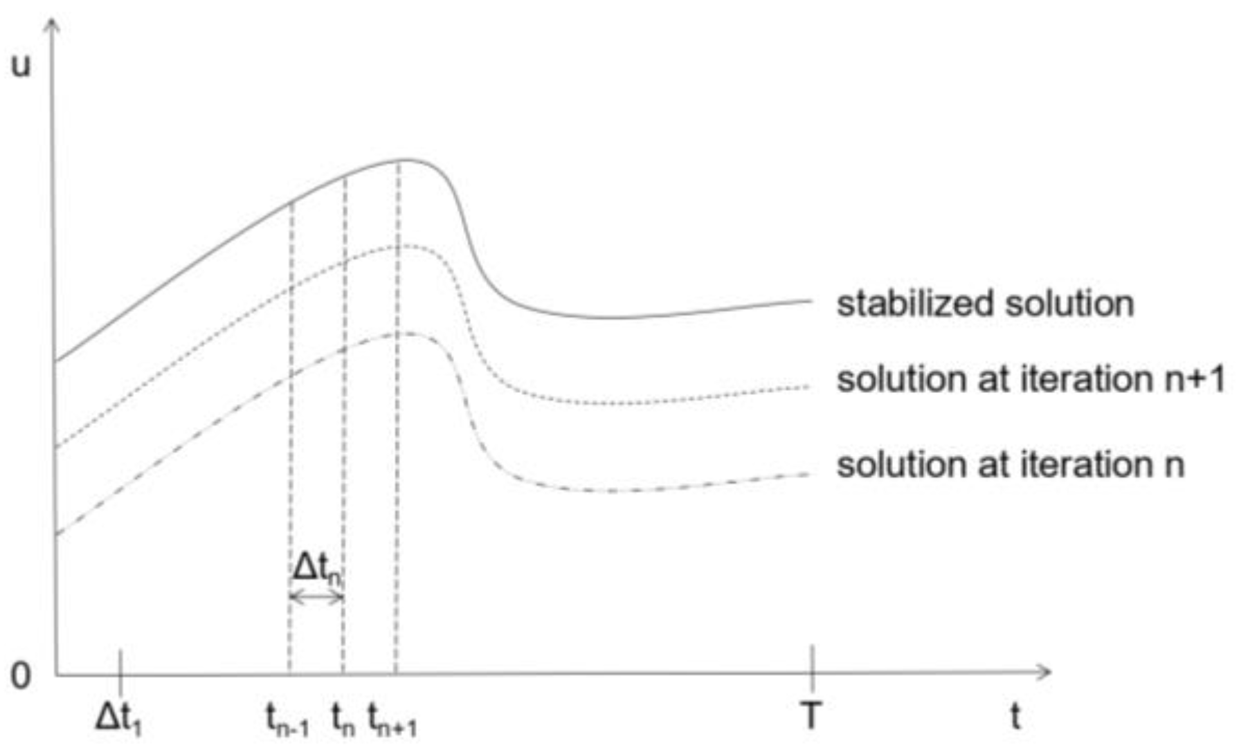
4.1. Direct Cyclic Technique

The direct cyclic method is used to simulate the RS of LCF. This is an effective modeling technique in Abaqus that can be used to obtain temperature and stress fields, saving time and costs. This technique is based on the construction of a displacement function to describe the response for all times (t) in a loading cycle of the period (T) (Figure 9).

The step utilizes the Fourier series,

$${\mathrm{u}\left(\mathrm{t}\right)=\mathrm{u}}_0+{\displaystyle \sum _{\mathrm{k}=1}^{\mathrm{n}}[}{\mathrm{u}}_k^s\sin \mathrm{k} \omega \mathrm{t}+{\mathrm{u}}_k^c\cos \mathrm{k} \omega \mathrm{t}]$$

(6)

where n is the number of terms in the Fourier series, ω is the angular frequency, and ${\mathrm{u}}_0$, ${\mathrm{u}}_k^s$ and ${\mathrm{u}}_k^{\mathrm{c}}$ are unknown displacement coefficients that can be calculated by the elastic stiffness matrix. In the following iterations, calculations are performed using revised displacement, rather than the previous displacements, until the stabilized response is obtained.

$$\mathrm{R}\left(\mathrm{t}\right)={\mathrm{R}}_0+{\displaystyle \sum _{\mathrm{k}=1}^{\mathrm{n}}[}{R}_k^s\sin \mathrm{k} \omega \mathrm{t}+R_k^c\cos \mathrm{k} \omega \mathrm{t}]$$

(7)

where the residual vector coefficient $R_0$, ${\mathrm{R}}_k^s$ and ${\mathrm{R}}_k^{\mathrm{c}}$ in the Fourier series corresponds to a displacement coefficient ${\mathrm{u}}_0$, ${\mathrm{u}}_k^s$ and ${\mathrm{u}}_k^{\mathrm{c}}$, respectively. The residual vector coefficients are obtained by tracking through the entire loading cycle. At each instant in time in the cycle, Abaqus obtains the residual vector R(t) by using standard element-by-element calculations,

$$R_0=\frac{2}{T}{\displaystyle {\int }_0^{T}R(t)dt}$$

(8)

$$R_k^s=\frac{2}{T}{\displaystyle {\int }_0^{T}R(t)\sin k\omega tdt}$$

(9)

$$R_k^c=\frac{2}{T}{\displaystyle {\int }_0^{T}R(t)\cos k\omega tdt}$$

(10)

The displacement solution is obtained by solving corrections to the displacement Fourier coefficients that correspond to each residual vector coefficient. The updated displacement solution is used in the next iteration to obtain the displacements at each instant in time. This process is repeated until the stabilized state is obtained.

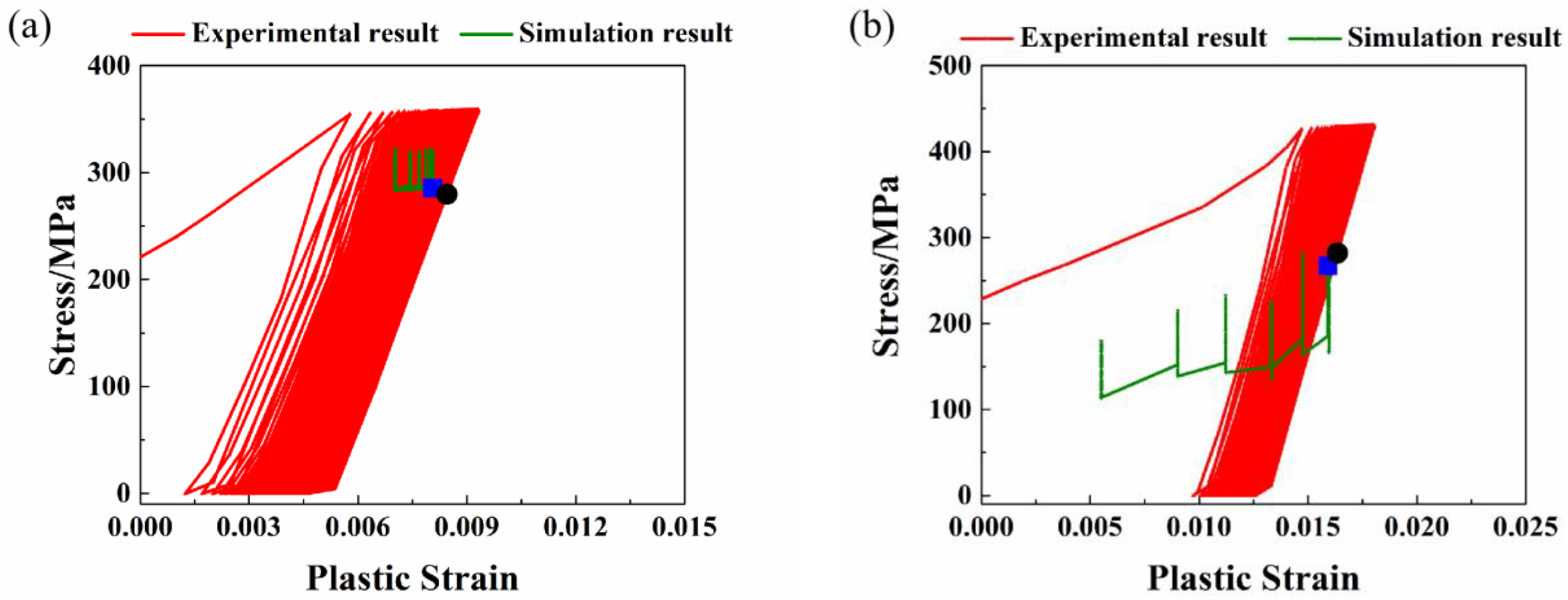
4.2. Combined Hardening Model

The hardening criterion addresses changes in the position and shape of the subsequent yield surface in stress space and describes them as deformation after the material enters the yield. It is related to the stress state, plastic strain, and hardening parameters. The existing hardening models are divided into three main types: isotropic hardening, kinematic hardening, and combined hardening. Different hardening models are selected for simulation and analysis, and the results show significant differences. In this paper, the Bauschinger effect occurs as C_N increases. Therefore, the isotropic hardening model is only used for the simulation of the RS of LW, whereas the combined hardening model is employed for the simulation of the RS of LCF. The combined hardening model allows the yield surface to expand and simultaneously translate, and is generally applied to the description of cyclic plasticity. The isotropic hardening component defines the size of the yield surface as a function of plastic deformation. The kinematic hardening component describes the translation of the yield surface in stress space through the backstress. The yield surface is defined by the function:

$$f(\sigma -\alpha )={\sigma }_{\mathrm{y}}$$

(11)

where f(σ – α) is the equivalent Mises stress, with respect to the backstress α.

5. Results and Discussions

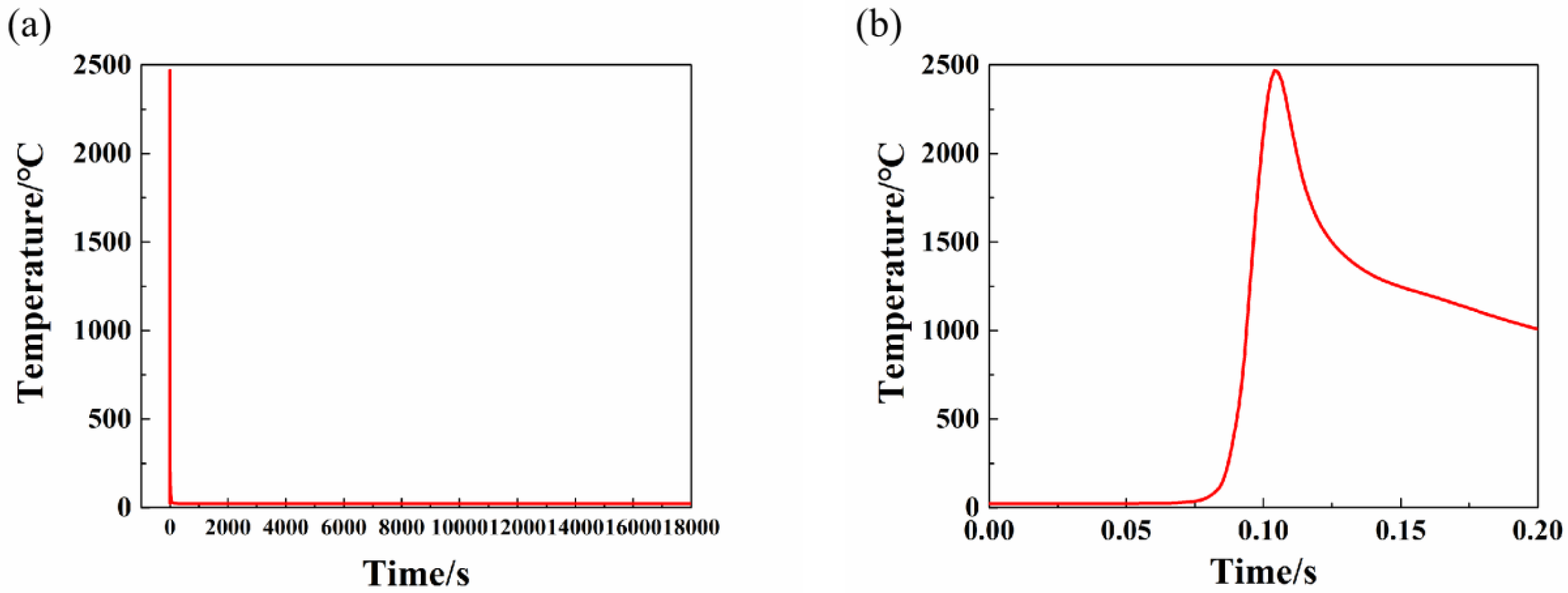
5.1. Temperature Field

Comparing the simulation cross-section with experimental results shows that there is a good match between them for the shape of the weld (Figure 10). The upper and lower surfaces of the half weld in the simulation are approximately 1.27 mm and 1.03 mm, while the experimental values are approximately 1.30 mm and 1.05 mm. The deviations of measurement and simulation are by factors such as molten pool flow, phase change, and keyhole vaporization, which are neglected in this study. The accuracy of the heat source model and parameter selection provides a foundation for the simulation of RS in the subsequent step.

Figure 11 shows the temperature change curve of the weld centre point during the LW process. When the heating time is less than 0.1 s, the temperature is room temperature. When the heating time is 0.1 s, due to the irradiation of the laser spot, the temperature rises rapidly in a short period to reach the peak of 2490 °C, and the temperature along the weld penetration direction also exceeds the melting point (1500 °C) [32]. When the heating time is more than 0.1 s, the temperature drops rapidly to room temperature, after the laser spot leaves.

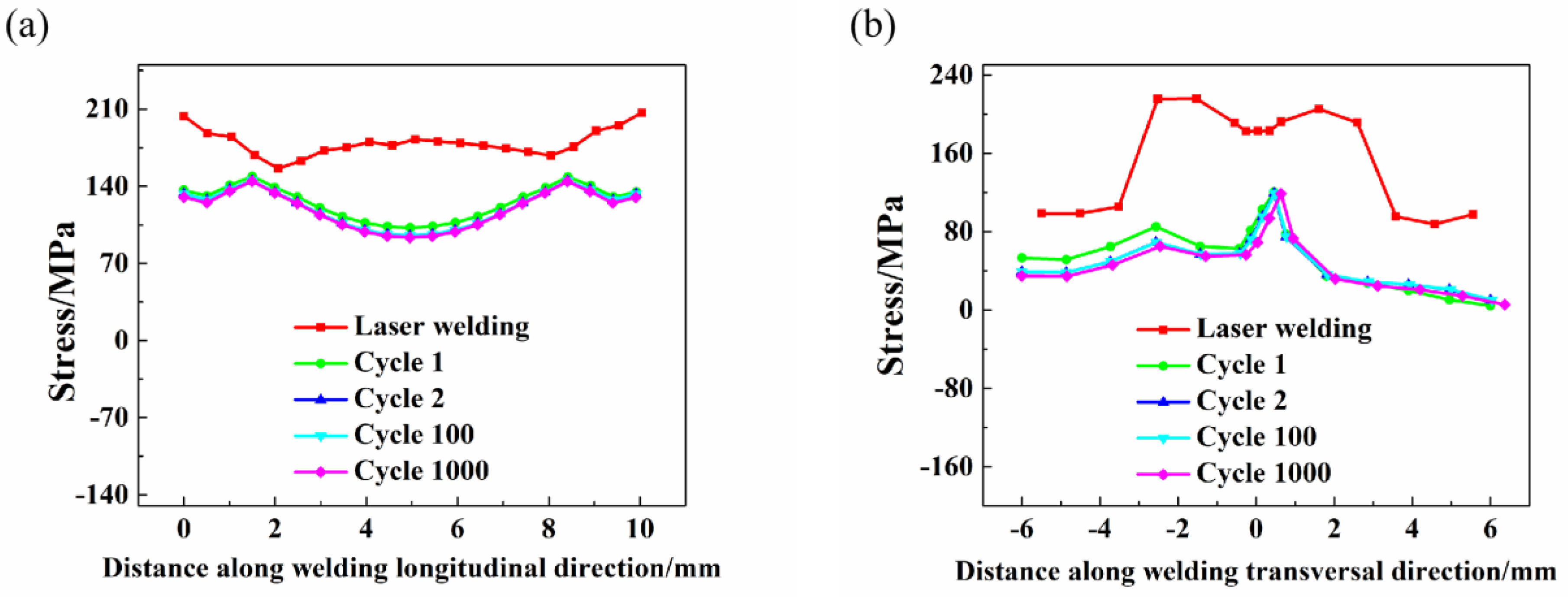
5.2. Residual Stress Relaxation

RS redistributes and relaxes after LCF, and usually occurs in the weld and heat-affected zone. When the welded structure has a fixed end and is applied cyclic loading on the other end. The cyclic loading and RS will be superposed, and the localized summed stress within the welded structure will equal or even exceed σ_y, resulting in macroscopic plastic deformation. In cases where the summed stress is lower than σ_y or does not lead to macroscopic plastic deformation, RS relaxation is attributed to the microscopic plastic process. RS relaxation is associated with the increased dislocation and vacancy of the crystal during LCF [14]. The summed stress causes dislocation movement in local areas of the welded structure. The crystal slips once the dislocation overcomes the internal resistance, which causes microscopic plastic deformation inside the crystal. The welded structure experiences secondary deformation after the cyclic loading is removed, and the accumulation of macroscopic or microscopic plastic strain results in redistribution and RS relaxation [10].

5.2.1. Influencing Factors of Residual Stress Relaxation

The RS relaxation caused by cyclic loading is mainly influenced by various factors, including the initial magnitude of RS, C_M and C_N, the cyclic σ-ε response of the material, and the degree of cyclic strain hardening or softening [33,34]. This paper focuses on investigating RS relaxation for different C_M and C_N, especially within the initial few cycles, which is why crack damage or fracture criteria are not included in the numerical simulation.

Figure 12 shows the longitudinal and transversal RS of LW and LCF curves with different C_M values (C_N is equal to 1000). RS relaxes in the weld and heat-affected zone, gradually increasing as C_M increases. When C_M exceeds σ_y of the material, the welded structure experiences significant deformation. The plastic deformation determines how much RS relaxation occurs, and the plastic deformation depends on C_M [35]. The RS only relaxes in the weld when C_M reaches 300 MPa, and the summed stress, which includes the RS of LW and the cyclic loading, is close to σ_y. However, when C_M increases to 400 or 500 Mpa, the summed stress also increases. Higher cyclic loading induces plastic flow, which changes the local constraints of RS, leading to redistribution and increased RS relaxation. This phenomenon can be explained by continuum mechanics. In addition, several research studies of welded structures have illustrated that RS relaxes more rapidly in the same direction as the cyclic loading (transversal direction). In practice, the stress along the transversal direction of the weld is therefore usually of more concern [36].

Figure 13 shows the longitudinal and transversal RS of LW and LCF curves with different C_N values (C_M is equal to 400 MPa). RS likewise relaxes in the weld and heat-affected zone, and relaxation occurs immediately after the first cycle. For the cyclic loading of 400 N, a relaxation of 44%, from 183 Mpa to 102 Mpa, is observed at the weld center. This relaxation is referred to as “quasi-static relaxation” and is generally detrimental to N_f improvement [34]. The degree of RS relaxation is more significant in the first few cycles. As C_N increases, the RS of LCF decreases slightly and then remains stable [37]. It is noteworthy that, in some cases, the RS can relax by more than 50% after the first cycle. The RS can even be relaxed entirely within the first few cycles [33].

5.2.2. Comparison of Experiment and Simulation

The comparative cyclic σ-ε curves obtained by the direct cyclic method and LCF experiment for different C_M are shown in Figure 14 (C_N is equal to 500). And the comparative cyclic σ-ε curves obtained by the direct cyclic method and LCF experiment for different C_N are shown in Figure 15 (C_M is equal to 400 MPa). Figure 14 and Figure 15 show reasonable agreement between the simulation and experimental results. The red curves in Figure 14 and Figure 15 are the cyclic σ-ε curves obtained from LCF experiments, with the black circles representing the stabilized stress and strain values; the green σ-ε curves are simulated by the direct cyclic method in Abaqus, with the blue squares representing the stabilized stress and strain values. It can be seen that the errors between the experiment and simulation decrease with increases in C_M and C_N, and that the stabilized stress and strain values are almost the same.

5.2.3. Residual Stress Relaxation Model

Based on the empirical equations, RS relaxation as the function of C_M and C_N is proposed in conjunction with creep behaviour. In order to analyze the relaxation law of RS, it is essential to understand the evolution of RS at different weld locations. RS along the longitudinal direction of the weld is measured, extending from 0 mm at the centre to 5 mm away from the centre. The RS curve is shown in Figure 16.

Figure 16 shows that when C_N is constant, RS relaxation in the weld centre is flat, and relaxation increases as distance increases. Moreover, RS relaxation in the weld centre is most apparent when C_M is constant, and decreases with increasing distance. The measurement values at 5 mm differ from others because the measurement errors are significant at the upper edge of the weld. Re is defined as the RS relaxation rate (0% < Re < 100%). Re at 0 mm is analyzed by referring to different C_M and C_N (Figure 17). C_N in Figure 17a is 1000, and C_M in Figure 17b is 400 MPa.

$$\mathrm{Re}=\frac{{\sigma }_{Laser}-{\sigma }_N}{{\sigma }_{Laser}}\times 100\%$$

(12)

where σ_Laser is the RS of LW and σ_N is the RS after N cycles. When Re is larger, relaxation is greater.

RS relaxation is similar to creep, in that both are material properties with unified mechanisms but different forms, and involve change in the deformation of the material over time when subject to applied loading or stress. The two phenomena interact with each other and have a specific conversion relationship. Creep is the phenomenon in which the strain of the material increases over time under constant loading. The corresponding RS relaxation refers to the process by which the stress on the material decreases over time. During creep, plastic deformation causes a change in the original residual stress distribution. As creep proceeds, the original higher RS region may decrease due to plastic deformation, while the original lower stress region may increase due to stress redistribution. At the same time, RS also affects the creep behavior. Higher RS may accelerate the creep process because the RS provides an additional driving force to plastic flow. Creep is dominated by diffusion at low temperatures and low stresses and dislocations at high temperatures and high stresses. In contrast, RS relaxation is mainly caused by dislocations at different temperatures [38]. On the basis of the above theory, RS relaxation model is proposed in this paper based on the creep model.

The equation for creep strain rate can be simplified in accordance with [36]:

$$\frac{\mathrm{d}\epsilon }{dt}=A{\sigma }^n$$

(13)

where ε is the strain, t is the time, σ is the stress, n is the stress index of the material, and A is the material constant.

Correspond the Re to ε and N to t. Since RS relaxation is related to σ_y [15], the ratio of cyclic loading (σ_cyclic) to σ_y corresponds to σ. Furthermore, introduce a constant (c) as a correction term. Equation (13) can be applied to RS relaxation. The modified equation is as follows:

$$\frac{dR\mathrm{e}}{df(N)}=\mathrm{g}({\sigma }_{\mathrm{cy}clic})=a{(\frac{{\sigma }_{\mathrm{cy}clic}}{{\sigma }_y})}^b+c$$

(14)

where f(N) is the function of cycle numbers, and a and b are the material constants.

$$f(N)=d\log {(N+1)}^e$$

(15)

In summary, the relationship between relaxation rate and C_M and C_N can be expressed as:

$$R\mathrm{e}=\left[a{(\frac{{\sigma }_{cyclic}}{{\sigma }_y})}^b+c\right]·d\log {(N+1)}^e$$

(16)

In Figure 17b, the relationship between Re and C_N is obtained by the same C_M (Equation (17) and Figure 18).

$$f(N)=0.19\log {(N+1)}^{0.05}$$

(17)

In Figure 17a, the equation between Re and C_M can be fitted (Equation (18) and Figure 19).

$$\mathrm{g}({\sigma }_{\mathrm{cy}clic})=1.407\times {(\frac{{\sigma }_{\mathrm{cy}clic}}{{\sigma }_y})}^{1.716}-0.5184$$

(18)

In summary, on the basis of Equation (16), RS relaxation can be expressed by Equation (19) and Figure 20.

$$R\mathrm{e}=\left[1.407\times {(\frac{{\sigma }_{cyclic}}{{\sigma }_y})}^{1.716}-0.5184\right]·\left[0.19\log {(N+1)}^{0.05}\right]$$

(19)

Two sets of parameters are randomly selected to verify the accuracy of the relaxation model. (1) cyclic loading of 350 MPa with 800 cycles, (2) cyclic loading of 450 MPa with 300 cycles. When C_N are 300 and 800, the effects of C_N on RS relaxation are predicted by the proposed Equation (17). When C_M are 350 MPa and 450 MPa, the relaxation of RS is calculated using the proposed Equation (18). The results show that Re obtained by the equations are 12.03% and 23.93%, and Re calculated by simulation are 11.40% and 23.72%, respectively. In summary, Equation (19) accounts for the effects of C_M and C_N on RS relaxation, producing results that agree well with the simulation data. The correctness of the relaxation model can be determined.

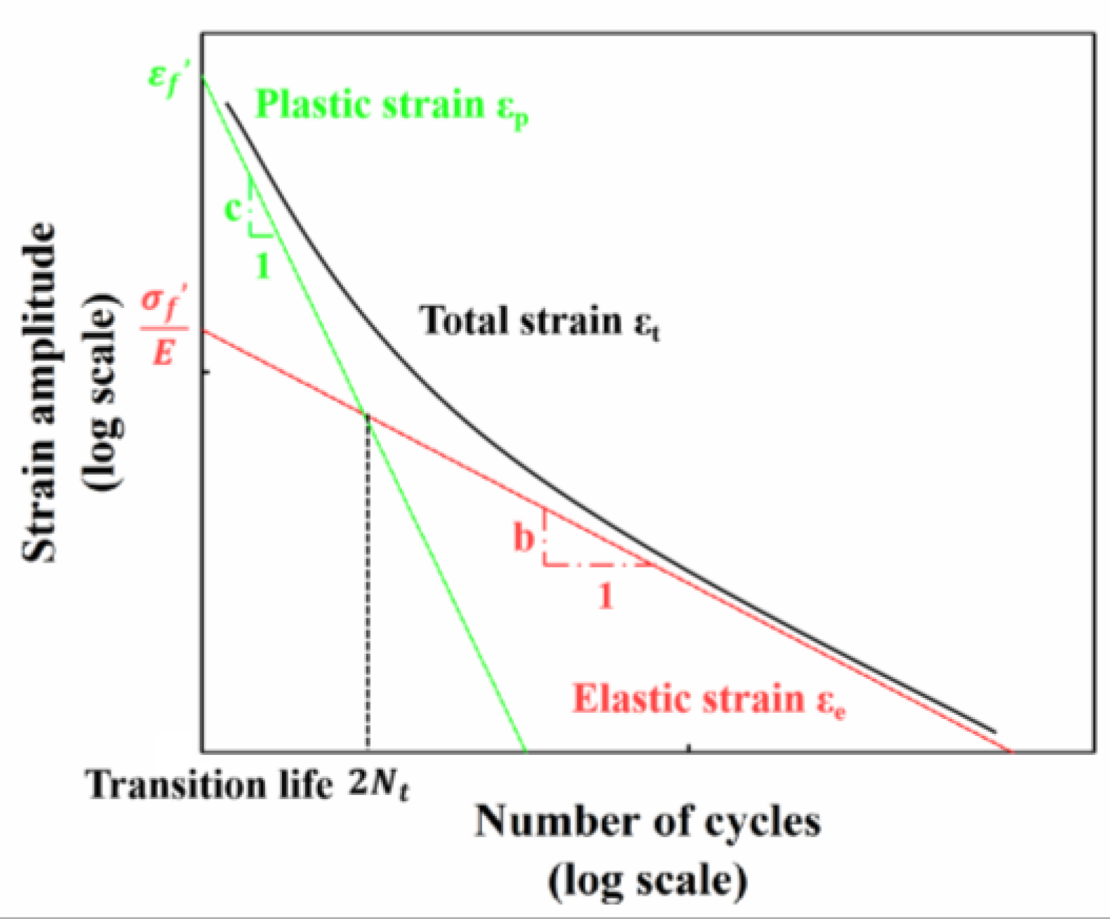
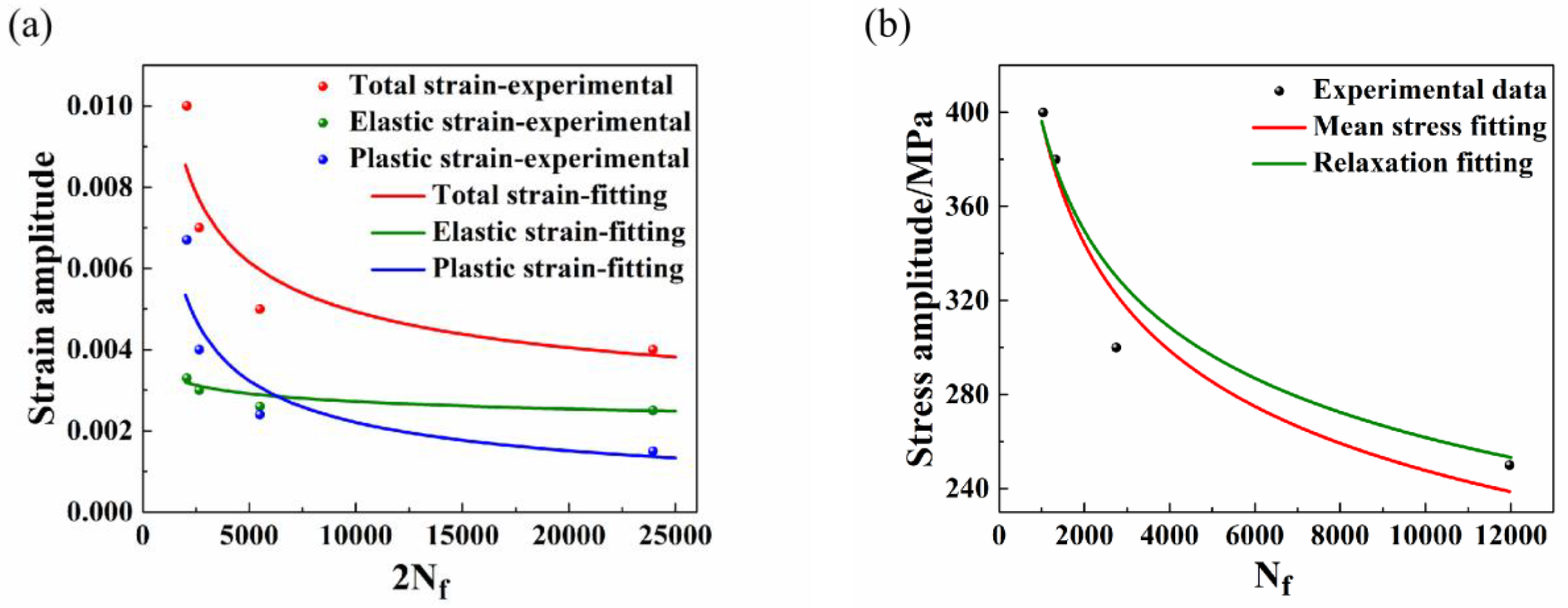
5.3. Fatigue Life Prediction Model

N_f prediction of the welded structure is considered to be a mature field that is based on numerous experimental and simulation studies [39]. However, many factors can influence N_f, such as welded structure dimension, temperature, multi-axial stress state, RS, σ_m, and crack, making it difficult to determine N_f accurately [11]. A large part of this uncertainty comes from RS.

The classical Basquin [40] (Equation (20)) and Coffin-Manson equations [41] (Equation (21)) are usually used to predict N_f. The Basquin model characterizes the relation between elastic strain amplitude and cycle numbers to failure.

$${\epsilon }_{\mathrm{e}}=\frac{{{\sigma }_f}^{\prime }}{E}{(2N_f)}^b$$

(20)

where ε_e is the elastic strain amplitude, σ_f′ is the fatigue strength, and b is the fatigue strength exponent [42]. The fatigue constants are obtained using regression analysis. The higher the value of σ_f′ and the smaller the absolute value of b (always negative), the longer the N_f [43]. Plastic strain amplitude and cycle numbers to failure are expressed by the Coffin-Manson model.

$${\epsilon }_{\mathrm{p}}={{\epsilon }_f}^{\prime }{(2N_f)}^c$$

(21)

where ε_p is the plastic strain amplitude, ε_f′ is the fatigue ductility coefficient, and c is the fatigue ductility exponent [42].

As shown in Figure 21, the elastic strain significantly affects N_f above the transition life (N_t). The plastic strain has a substantial influence on N_f below N_t. Therefore, N_t delineates LCF and high-cycle fatigue. Since the welded structure rarely experiences completely reversed cyclic loading in practical applications, service cyclic loading can result in the presence of the mean strain or stress. Landgraf proposed introducing σ_m into the N_f estimation [44], and so Equation (20) is modified as follows:

$${\epsilon }_{\mathrm{e}}=\frac{{{\sigma }_f}^{\prime }-{\sigma }_m}{E}{(2N_f)}^b$$

(22)

During LCF, RS may be present in the welded structure in the form of tensile or compressive σ_m [45]. The properties of the welded structure after LCF are negatively impacted by mean tensile stress. On the contrary, mean compressive stress has favourable effects on the fatigue properties. However, as mentioned above, RS redistributes and relaxes during LCF. When predicting N_f, it is inaccurate to consider RS or σ_m as the constant. Therefore, the RS relaxation model proposed in this paper is introduced into the Basquin and Coffin-Manson N_f prediction equation.

$${\epsilon }_{\mathrm{e}}=\frac{{{\sigma }_f}^{\prime }-{\sigma }_{Laser}·(1-\mathrm{Re})}{E}{(2N_f)}^b$$

(23)

Since the RS of LCF relaxes rapidly after the first cycle and remains stable, N is equal to 1 in Equation (19).

N_f under different C_M can be obtained by LCF experiments. Equations (20)–(23) can be fitted by experimental data and the results are shown in

Table 3. Parameters of N_f models.

	σf′	b	εf′	c	R2
Equations (20) and (21)	1607	−0.10	0.35	−0.55	74.62%
Equation (22)	1875	−0.20			92.79%
Equation (23)	1758	−0.18			98.08%

and Figure 22. By comparing the N_f calculated by equations, the error R² can be used to estimate the accuracy of the N_f prediction model proposed in this paper.

Table 3 and Figure 22 show the R² of Equation (23) is larger than Equations (20)–(22), indicating that the N_f model, which considers RS relaxation, can better fit the experimental data. Meanwhile, the N_f model that does not consider RS or relaxation phenomena will overestimate N_f, and the N_f model that considers RS as σ_m will underestimate N_f.

6. Conclusions

This paper reports an experimental and simulated effort to address residual stress. The residual stress of laser welding is studied by establishing the sequential-coupled thermal-mechanical model. The residual stress of low-cycle fatigue is simulated by using the direct cyclic method and combined hardening model, and the relaxation and redistribution of residual stress are found. Furthermore, the residual stress relaxation model is proposed by comparing residual stress evolution in different cyclic loading and number of cycles. On this basis, fatigue life is predicted, and the effects of residual stress relaxation on fatigue life are found. The simulation results are verified by the experimental data for low-cycle fatigue and neutron diffraction, which show good agreement. The work undertaken in this study supports the following conclusions:

(1)

The thermal analysis demonstrates that the finite element simulation results of the temperature history distribution that are measured in the weld and heat-affected zone agree with the experimental results.

(2)

Plastic material constitutive models, combined hardening model, and the direct cyclic method can accurately investigate the residual stress of laser welding and low-cycle fatigue. The simulated results are verified by neutron diffraction experimental results with a similar distribution and magnitude.

(3)

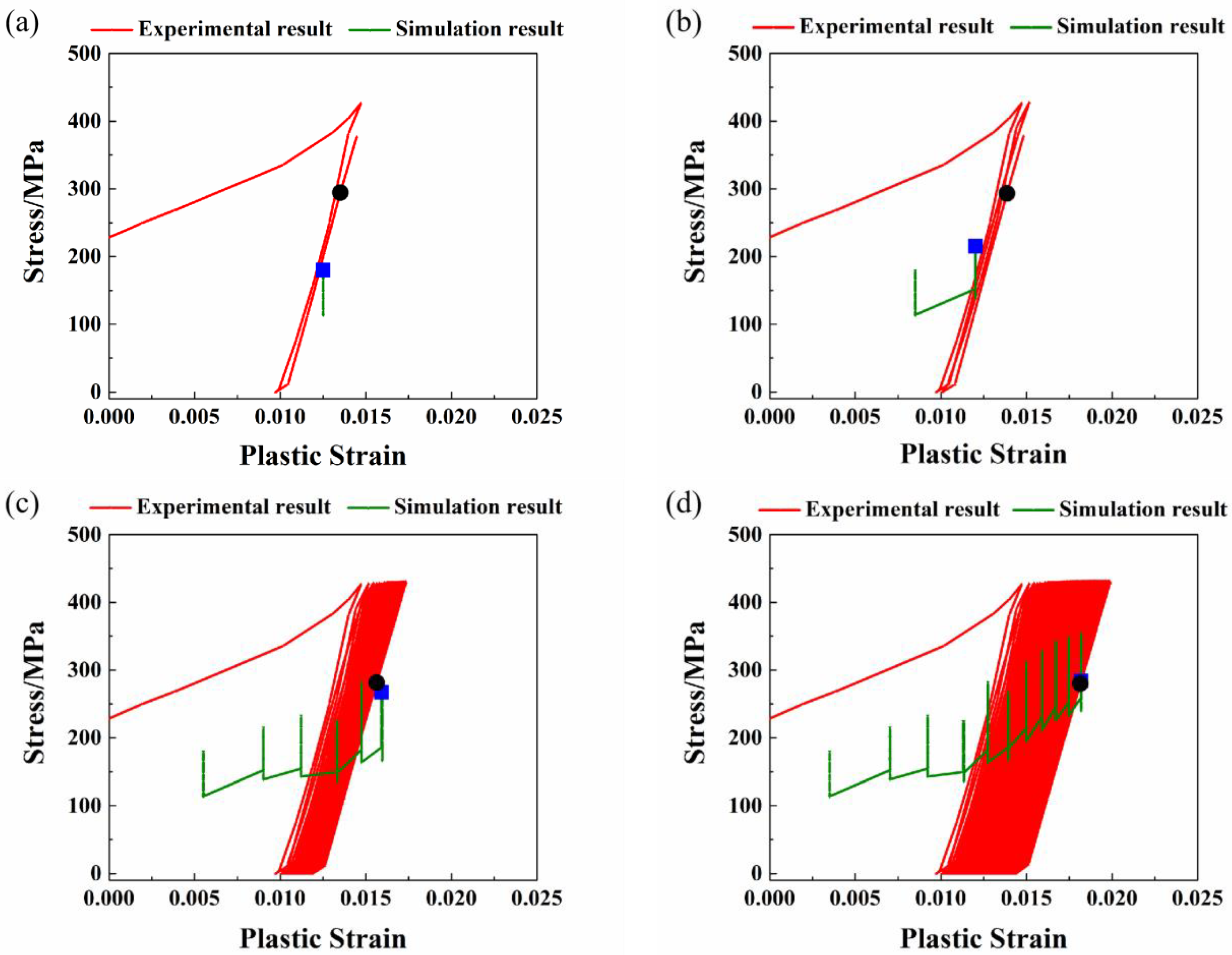
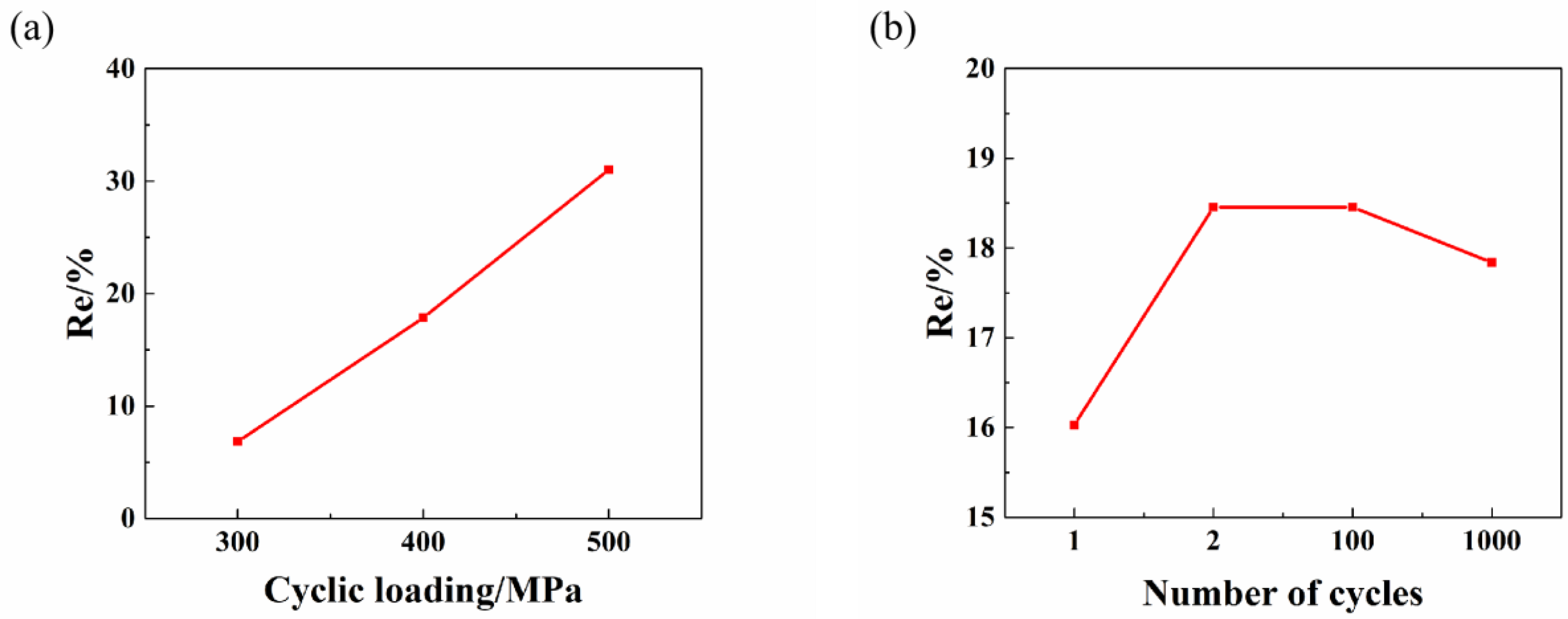
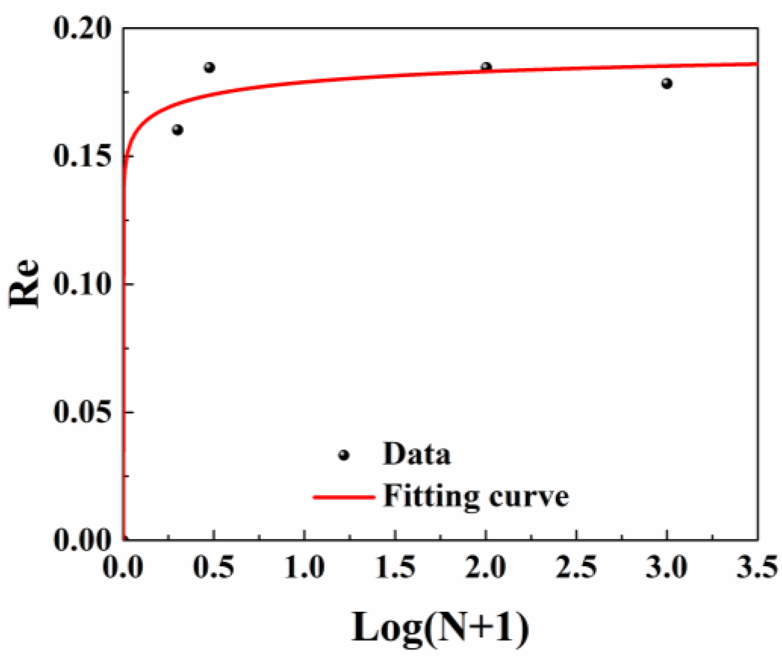
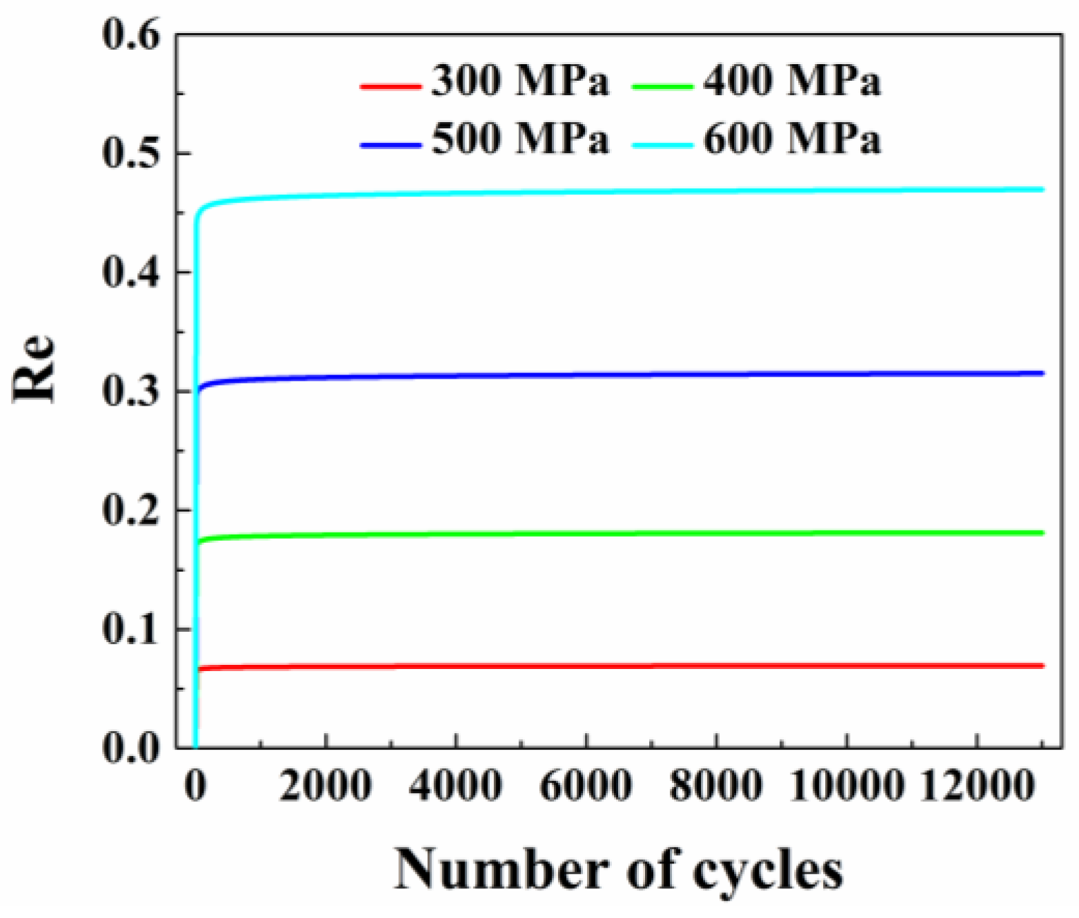
After low-cycle fatigue, residual stress redistributes and relaxes in the weld and heat-affected zone. The most significant relaxation happens within the first cycle. The amount of residual stress relaxation depends on cyclic loading and the number of cycles. This study proposes the residual stress relaxation model by comparing the evolution of residual stress in relation to two influenced factors. The relaxation model can represent the change process of residual stress well by providing data verification.

(4)

Fatigue life is significantly influenced by residual stress and relaxation behavior. This paper proposes an improved fatigue life model that is based on the Basquin and Coffin-Manson fatigue life models. The above residual stress relaxation model is introduced into the fatigue life model to predict low-cycle fatigue life better.

References

1. Chen, Y.; Sun, S.; Zhang, T.; Zhou, X.; Li, S. Effects of post-weld heat treatment on the microstructure and mechanical properties of laser-welded NiTi/304SS joint with Ni filler. Mater. Sci. Eng. A 2020, 771, 138545. [Google Scholar] [CrossRef]
2. Mihaliková, M.; Zgodavová, K.; Bober, P.; Špegárová, A. The performance of CR180IF and DP600 laser welded steel sheets under different strain rates. Materials 2021, 14, 1553. [Google Scholar] [CrossRef] [PubMed]
3. Jeyaprakash, N.; Haile, A.; Arunprasath, M. The parameters and equipments used in TIG welding: A review. Int. J. Eng. Sci. 2015, 4, 11–20. [Google Scholar]
4. Idriss, M.; Mirakhorli, F.; Desrochers, A. Fatigue behaviour of AA5052-H36 laser-welded overlap joints: Effect of stitch-weld orientation and gap bridging. Int. J. Fatigue 2023, 167, 107358. [Google Scholar] [CrossRef]
5. Wallerstein, D.; Salminen, A.; Lusquiños, F.; Comesaña, R.; García, J.V.; Rodríguez, A.R.; Badaoui, A. Recent developments in laser welding of aluminum alloys to steel. Metals 2021, 11, 622. [Google Scholar] [CrossRef]
6. Zhang, Y.; You, D.; Gao, X.; Zhang, N.; Gao, P.P. Welding defects detection based on deep learning with multiple optical sensors during disk laser welding of thick plates. J. Manuf. Syst. 2019, 51, 87–94. [Google Scholar] [CrossRef]
7. Wang, X.; Meng, Q.; Hu, W. Numerical analysis of low cycle fatigue for welded joints considering welding residual stress and plastic damage under combined bending and local compressive loads. Fatigue Fract. Eng. Mater. Struct. 2020, 43, 1064–1080. [Google Scholar] [CrossRef]
8. Rossini, N.S.; Dassisti, M.; Benyounis, K.Y.; Olabi, A.G. Methods of measuring residual stresses in components. Mater. Des. 2012, 35, 572–588. [Google Scholar] [CrossRef]
9. Paul, S.K.; Stanford, N.; Taylor, A.; Hilditch, T. The effect of low cycle fatigue, ratcheting and mean stress relaxation on stress-strain response and microstructural development in a dual phase steel. Int. J. Fatigue 2015, 80, 341–348. [Google Scholar] [CrossRef]
10. Wang, X.; Meng, Q.; Hu, W. Fatigue life prediction for butt-welded joints considering weld-induced residual stresses and initial damage, relaxation of residual stress, and elasto-plastic fatigue damage. Fatigue Fract. Eng. Mater. Struct. 2019, 42, 1373–1386. [Google Scholar] [CrossRef]
11. Zhiping, Q.; Zesheng, Z.; Lei, W. Numerical analysis methods of structural fatigue and fracture problems. Contact Fract. Mech. 2018, 12, 235. [Google Scholar]
12. Hao, H.; Ye, D.; Chen, Y.; Feng, M.; Liu, J. A study on the mean stress relaxation behavior of 2124-T851 aluminum alloy during low-cycle fatigue at different strain ratios. Mater. Des. 2015, 67, 272–279. [Google Scholar] [CrossRef]
13. Hossain, M.; Ziehl, P. Modelling of Fatigue Crack Growth with Abaqus; University of South Carolina: Columbia, SC, USA, 2012. [Google Scholar]
14. Chakherlou, T.N.; Yaghoobi, A. Numerical simulation of residual stress relaxation around a cold-expanded fastener hole under longitudinal cyclic loading using different kinematic hardening models. Fatigue Fract. Eng. Mater. Struct. 2010, 33, 740–751. [Google Scholar] [CrossRef]
15. You, C.; Achintha, M.; Soady, K.A. Low cycle fatigue life prediction in shot-peened components of different geometries-part I: Residual stress relaxation. Fatigue Fract. Eng. Mater. Struct. 2017, 40, 761–775. [Google Scholar] [CrossRef]
16. Morrow, J.; Sinclair, G.M. Cycle-Dependent Stress Relaxation; ASTM International: West Conshohocken, PA, USA, 1958. [Google Scholar]
17. Jhansale, H.R.; Topper, T.H. Engineering Analysis of the Inelastic Stress Response of a Structural Metal under Variable Cyclic Strains. Cyclic Stress-Strain Behavior Analysis, Experimentation, and Failure Prediction; ASTM International: West Conshohocken, PA, USA, 1973; pp. 246–270. [Google Scholar]
18. Kodama, S. The behavior of residual stress during fatigue stress cycles. Soc. Mater. Sci. 1972, 2, 111–118. [Google Scholar]
19. Holzapfel, H.; Schulze, V.; Vöhringer, O. Residual stress relaxation in AISI 4140 steel due to quasistatic and cyclic loading at higher temperatures. Mater. Sci. Eng. A 1998, 248, 9–18. [Google Scholar] [CrossRef]
20. Hemmesi, K.; Mallet, P.; Farajian, M. Numerical evaluation of surface welding residual stress behavior under multiaxial mechanical loading and experimental validations. Int. J. Mech. Sci. 2020, 168, 105–127. [Google Scholar] [CrossRef]
21. Derakhshan, E.D.; Yazdian, N.; Craft, B.; Smith, S. Numerical simulation and experimental validation of residual stress and welding distortion induced by laser-based welding processes of thin structural steel plates in butt joint configuration. Opt. Laser Technol. 2018, 104, 170–182. [Google Scholar] [CrossRef]
22. Liu, M.; Kouadri-Henni, A.; Malard, B. Numerical analysis of low-cycle fatigue using the direct cyclic method considering laser welding residual stress. Coatings 2023, 13, 553. [Google Scholar] [CrossRef]
23. Rosado-Carrasco, J.G.; González-Zapatero, W.F. Analysis of the low cycle fatigue behavior of DP980 steel gas metal arc welded joints. Metals 2022, 12, 419. [Google Scholar] [CrossRef]
24. Farabi, N.; Chen, D.L.; Li, J.; Zhou, Y.; Dong, S.J. Microstructure and mechanical properties of laser welded DP600 steel joints. Mater. Sci. Eng. A 2010, 527, 1215–1222. [Google Scholar] [CrossRef]
25. Rahmaan, T.; Bardelcik, A.; Imbert, J.; Butcher, C. Effect of strain rate on flow stress and anisotropy of DP600, TRIP780, and AA5182-O sheet metal alloys. Int. J. Impact Eng. 2016, 88, 72–90. [Google Scholar] [CrossRef]
26. ASTM E606; Standard Practice for Strain-Controlled Fatigue Testing. ASTM: West Conshohocken, PA, USA, 1998; Volume 3.
27. Marciszko, M. Diffraction Study of Mechanical Properties and Residual Stresses Resulting from Surface Processing of Polycrystalline Materials; AGH University of Science and Technology in Kraków: Kraków, Poland, 2013. [Google Scholar]
28. Avettand-Fènoël, M.N.; Sapanathan, T.; Pirling, T. Investigation of residual stresses in planar dissimilar magnetic pulse welds by neutron diffraction. J. Manuf. Process 2021, 68, 1758–1766. [Google Scholar] [CrossRef]
29. Kim, J.C.; Cheong, S.K.; Noguchi, H. Residual stress relaxation and low-and high-cycle fatigue behavior of shot-peened medium-carbon steel. Int. J. Fatigue 2013, 56, 114–122. [Google Scholar] [CrossRef]
30. Sowards, J.W.; Pfeif, E.A.; Connolly, M.J.; McColskey, J.D. Low-cycle fatigue behavior of fiber-laser welded, corrosion-resistant, high-strength low alloy sheet steel. Mater. Des. 2017, 121, 393–405. [Google Scholar] [CrossRef]
31. Yilbas, B.S.; Akhtar, S. Laser welding of AISI 316 steel: Microstructural and stress analysis. J. Manuf. Sci. Eng. 2013, 135, 031018. [Google Scholar] [CrossRef]
32. Wan, X.; Wang, Y.; Zhang, P. Modelling the effect of welding current on resistance spot welding of DP600 steel. J. Mater. Process Technol. 2014, 214, 2723–2729. [Google Scholar] [CrossRef]
33. Zhuang, W.Z.; Halford, G.R. Investigation of residual stress relaxation under cyclic load. Int. J. Fatigue 2001, 23, 31–37. [Google Scholar] [CrossRef]
34. Zaroog, O.S.; Ali, A.; Sahari, B.B.; Zahari, R. Modeling of residual stress relaxation of fatigue in 2024-T351 aluminium alloy. Int. J. Fatigue 2011, 33, 279–285. [Google Scholar] [CrossRef]
35. Wang, L.; Qian, X. Welding residual stresses and their relaxation under cyclic loading in welded S550 steel plates. Int. J. Fatigue 2022, 162, 106992. [Google Scholar] [CrossRef]
36. Qian, Z.; Chumbley, S.; Karakulak, T.; Johnson, E. The residual stress relaxation behavior of weldments during cyclic loading. Metall. Mater. Trans. A 2013, 44, 3147–3156. [Google Scholar] [CrossRef]
37. Ferro, P. The local strain energy density approach applied to pre-stressed components subjected to cyclic load. Fatigue Fract. Eng. Mater. Struct. 2014, 37, 1268–1280. [Google Scholar] [CrossRef]
38. Valluri, S.R. Some recent developments at GALCIT concerning a theory of metal fatigue. Acta Metall. 1963, 11, 759–775. [Google Scholar] [CrossRef]
39. James, M.N.; Hughes, D.J.; Chen, Z.; Lombard, H. Residual stresses and fatigue performance. Eng. Fail. Anal. 2007, 14, 384–395. [Google Scholar] [CrossRef]
40. Basquin, O.H. The exponential law of endurance tests. Am. Soc. Test. Mater. Proc. 1910, 10, 625–630. [Google Scholar]
41. Coffin, L.F., Jr. A study of the effects of cyclic thermal stresses on a ductile metal. Trans. Am. Soc. Mech. Eng. 1954, 76, 931–949. [Google Scholar] [CrossRef]
42. Bassindale, C.; Miller, R.E.; Wang, X. Effect of single initial overload and mean load on the low-cycle fatigue life of normalized 300 M alloy steel. Int. J. Fatigue 2020, 130, 105273. [Google Scholar] [CrossRef]
43. Parkes, D.; Xu, W.; Westerbaan, D.; Nayak, S.S.; Zhou, Y. Microstructure and fatigue properties of fiber laser welded dissimilar joints between high strength low alloy and dual-phase steels. Mater. Des. 2013, 51, 665–675. [Google Scholar] [CrossRef]
44. Landgraf, R.W.; Chernenkoff, R.A. Residual Stress Effects on Fatigue of Surface Processed Steels; ASTM International: West Conshohocken, PA, USA, 1988; pp. 1–12. [Google Scholar]
45. Minamizawa, K.; Arakawa, J.; Akebono, H. Fatigue limit estimation for carburized steels with surface compressive residual stress considering residual stress relaxation. Int. J. Fatigue 2022, 160, 106846. [Google Scholar] [CrossRef]
Figure 1. The process of deep penetration welding.
Coatings 14 00281 g001
Figure 2. The platform of Nd: YAG laser.
Coatings 14 00281 g002
Figure 3. Dimensions of LCF specimens.
Coatings 14 00281 g003
Figure 4. One cyclic loading in the LCF experiment.
Coatings 14 00281 g004
Figure 5. (a) Cyclic σ-ε curve of 250 MPa, (b) Cyclic σ-ε curve of 300 Mpa, (c) Cyclic σ-ε curve of 380 Mpa, (d) Cyclic σ-ε curve of 400 Mpa, (e) Nf curve.
Coatings 14 00281 g005
Figure 6. The platform and specimen of LCF experiment.
Coatings 14 00281 g006
Figure 7. Schematic of ND experiment.
Coatings 14 00281 g007
Figure 8. The RS of LCF by ND experiment (a) Von Mises, (b) S1 and S2.
Coatings 14 00281 g008
Figure 9. Displacement function for all times t in a loading cycle of period T at different iterations.
Coatings 14 00281 g009
Figure 10. Simulation of weld cross-section.
Coatings 14 00281 g010
Figure 11. Temperature curve of the weld center point (a) welding and cooling processes, (b) welding process.
Coatings 14 00281 g011
Figure 12. The RS of LW and LCF with different CM (a) longitudinal, (b) transversal.
Coatings 14 00281 g012
Figure 13. The RS of LW and LCF with different CN (a) longitudinal, (b) transversal.
Coatings 14 00281 g013
Figure 14. Cyclic σ-ε curve obtained by the direct cyclic method and LCF experiment (a) 300 MPa, (b) 400 Mpa.
Coatings 14 00281 g014
Figure 15. Cyclic σ-ε curve obtained by the direct cyclic method and LCF experiment (a) 1 cycle, (b) 2 cycles, (c) 100 cycles, (d) 1000 cycles.
Coatings 14 00281 g015
Figure 16. RS curve of the weld in a longitudinal direction (a) CM, (b) CN.
Coatings 14 00281 g016
Figure 17. RS relaxation rate (a) CM, (b) CN.
Coatings 14 00281 g017
Figure 18. Fitting curves of CN.
Coatings 14 00281 g018
Figure 19. Fitting curves of CM.
Coatings 14 00281 g019
Figure 20. Relaxation rate with different CM and CN.
Coatings 14 00281 g020
Figure 21. Basquin and Coffin-Manson curve.
Coatings 14 00281 g021
Figure 22. Experimental data and fitting curves of Nf models (a) Basquin and Coffin-Manson, (b) σm and RS relaxation.
Coatings 14 00281 g022