A Reduced-Order FEM Based on POD for Solving Non-Fourier Heat Conduction Problems under Laser Heating

Abstract

The study presents a novel approach called FEM-POD, which aims to enhance the computational efficiency of the Finite Element Method (FEM) in solving problems related to non-Fourier heat conduction. The present method employs the Proper Orthogonal Decomposition (POD) technique. Firstly, spatial discretization of the second-order hyperbolic differential equation system is achieved through the Finite Element Method (FEM), followed by the application of the Newmark method to address the resultant ordinary differential equation system over time, with the resultant numerical solutions collected in snapshot form. Next, the Singular Value Decomposition (SVD) is employed to acquire the optimal proper orthogonal decomposition basis, which is subsequently combined with the FEM utilizing the Newmark scheme to construct a reduced-order model for non-Fourier heat conduction problems. To demonstrate the effectiveness of the suggested method, a range of numerical instances, including different laser heat sources and relaxation durations, are executed. The numerical results validate its enhanced computational accuracy and highlight significant time savings over addressing non-Fourier heat conduction problems using the full order FEM with the Newmark approach. Meanwhile, the numerical results show that when the number of elements or nodes is relatively large, the CPU running time of the FEM-POD method is even hundreds of times faster than that of classical FEM with the Newmark scheme.

1. Introduction

The classical mathematical model for heat conduction, known as Fourier’s law, was established in 1822 to explain the relationship between heat flow and temperature. It postulates that the amount of heat passing through a particular segment in a given time period is directly proportional to the rate of temperature change and the cross-sectional area perpendicular to the direction of heat flow. This law has found extensive applications in traditional engineering thermal problems, such as determining U-tube heat transfer areas, investigating thermodynamics of automotive ventilation disc brakes, and developing insulation systems for cryogenic wind tunnels. However, Fourier’s law neglects the effects of inertia in the process of heat conduction and assumes an infinite rate of heat. For large-scale space and time conditions, its influence can be ignored. In most cases, the Fourier law is in excellent description of heat conduction physics because real heat propagation speeds are very high. Thus, assuming infinite speed is generally accurate and efficient. However, as emerging technologies continue to evolve (such as high-frequency laser heat source, nanocoating, etc.), researchers have found that the calculation error of Fourier’s law is large for the heat conduction problems under the conditions of extremely high (low) temperature, ultra-fast speed and micro-space or micro-time scale. In such scenarios, where temperature gradients are exceptionally high, the classical assumption of infinite heat propagation velocity no longer holds true. Consequently, an improved version of the Fourier law known as non-Fourier law has been developed to account for finite values of heat propagation velocity [1].

The occurrence of non-Fourier effect is typically observed under the following conditions: (a) when the spatial scale of thermal effect is extremely small, such as in nanotechnology; (b) when the thermal effect is exceptionally fast, for instance in ultra-fast laser heating; and (c) when the temperature of the heat conducting object approaches absolute zero. In practical research, the conditions of non-Fourier effect are extremely harsh, thus the cost and technical requirements of obtaining research results through experiments are high. However, the analytical method is applicable to a limited range and can only solve simple functional relations, and it is difficult to obtain the explicit expression for some complex boundary conditions. Hence, the utilization of numerical simulation has become pivotal in tackling non-Fourier heat conduction problems. Consequently, there has been a notable upsurge in scholarly attention towards the numerical resolution of such problems in recent years. Several numerical techniques, encompassing but not confined to the finite difference method (FDM) [2,3], the finite element method (FEM) [4,5,6], the finite difference method, finite volume method (FVM) [7], the boundary element method (BEM) [8,9], the meshless methods [1,10,11,12], and the lattice Boltzmann method [13,14], have been put forth to address these concerns.

The primary challenge in large-scale complex modeling lies in reducing computational costs while maintaining numerical accuracy. The prevalent and significant approaches involve altering the formulae through partial equation modifications or reducing the equation order. In contrast to the former, the reduced-order model is favored for its simplicity, efficiency, and widespread application, as it diminishes the degrees of freedom and transforms the computation of partial differential equations (PDEs) into linear equations within a lower-dimensional space [15]. Among the model reductions methods, the POD method, which is interchangeably known as Karhunen-Loève Decomposition (KLD), Principal Component Analysis (PCA), or SVD, provides an efficient way to extract a simplified, low-dimensional model from complex high-dimensional systems [16,17].

The technique offers several advantages as it allows for the representation of a physical process through a linear combination of orthogonal basis functions and amplitudes in a least-square optimal manner. Consequently, it is able to capture a greater amount of energy compared to other decomposition methods employing the same number of basis functions. Notably, the method is entirely data-dependent, making it suitable for modeling dynamic systems without any prior knowledge of the underlying process. This approach facilitates the creation of lower-order models that can potentially provide valuable insights into the generative process behind the data. Furthermore, the POD technique can be combined with a variety of numerical methods (such as FEM [17,18,19], FDM [18,20], FVM [21] meshless methods [16,22,23,24], etc.) to reduce the number of degrees of freedom in intricate problems and is widely used in reducing the dimension of partial differential equations. Although many scholars have used it to study Fourier heat conduction problems for heat transfer applications, there has been limited research on non-Fourier heat conduction problems. Therefore, this paper proposes using FEM combined with POD techniques to construct reduced-order models for non-Fourier heat conduction problems and discusses their feasibility under different laser heating sources and relaxation times.

The innovation of this work lies in combining the Proper Orthogonal Decomposition (POD) model order reduction method with the Finite Element Method (FEM), proposing a fast algorithm that improves computational efficiency. The characteristic of this method is that it can reduce the discretized equations from the FEM, which originally contain thousands of degrees of freedom, to just a few dozen degrees of freedom. This significantly improves computational efficiency while ensuring calculation accuracy.

2. Mathematical Model

Stemming from Fourier’s law of heat conduction, the traditional parabolic equation for heat conduction suggests a direct proportionality between the rate of heat transfer and the temperature gradient, that is,

$$\mathit{q}(\mathit{x},t)=-k\nabla \theta (\mathit{x},t),$$

(1)

where $\mathit{x}$ is the spatial coordinates, ∇ is the Nabla operator, k is the thermal conductivity coefficient, $\theta (\mathit{x},t)$ is the temperature at point $\mathit{x}\in \mathsf{\Omega }$ and at time t, $\mathit{q}$ is the heat flux. Experimental findings challenge the Fourier law, which states that thermal propagation velocity is infinite, suggesting its breakdown at decreasing feature sizes. Consequently, there has been considerable interest in non-Fourier heat transfer theory in the field of heat transfer research. Several non-Fourier models have been proposed, including the wave model. The hyperbolic heat conduction equation arises from this model. This paper considers the hyperbolic heat conduction equation based on the Cattaneo-Vernotte (CV) relation, which accounts for a time delay between the heat flux and the temperature gradient. It is as follows:

$$\mathit{q}(\mathit{x},t+\tau )=-k\nabla \theta (\mathit{x},t),$$

(2)

where $\tau$ represents the thermal relaxation time. This constitutive law assumes that heat flow and temperature gradient do not occur simultaneously. Obviously, if $\tau =0$, then Equation (2) becomes the Fourier thermal diffusion model (1).

In general, the heat flow is governed by the following conduction equation:

$$-\nabla ·\mathit{q}(\mathit{x},t)+Q(\mathit{x},t)=\rho c\frac{\theta (\mathit{x},t)}{\partial t},$$

(3)

where $Q(\mathit{x},t)$ represents a known internal heat source, $\rho$ denotes mass density, and c represents specific heat.

If the thermal relaxation time $\tau$ is small enough, with Equation (2), by applying a time-based first-order Taylor series expansion and disregarding the minor high-order quantity, one can achieve:

$$\mathit{q}(\mathit{x},t)+\tau \frac{\partial \mathit{q}(\mathit{x},t)}{\partial t}=-k\nabla \theta (\mathit{x},t).$$

(4)

Combining Equations (2) and (4) and eliminating $\mathit{q}$, yields

$$\tau \rho c\frac{{\partial }^2\theta (\mathit{x},t)}{\partial t^2}+\rho c\frac{\partial \theta (\mathit{x},t)}{\partial t}=k{\nabla }^2\theta (\mathit{x},t)+\tau \frac{\partial Q(\mathit{x},t)}{\partial t}+Q(\mathit{x},t),(\mathit{x},t)\in \mathsf{\Omega }\times J,$$

(5)

where $J=(0,T]$ is denoted as the time interval. Equation (5) is referred to as the thermal wave equation.

In general, the thermal wave equation Equation (5) must be solved for prescribed initial and boundary conditions. Here, the initial conditions are

$$\left\{\begin{array}{c}\theta (\mathit{x},0)={\theta }^0\left(\mathit{x}\right),\mathit{x}\in \mathsf{\Omega },\hfill \\ \frac{\partial \theta (\mathit{x},0)}{\partial t}=D^0\left(\mathit{x}\right),\mathit{x}\in \mathsf{\Omega },\hfill \end{array}\right.$$

(6)

where ${\theta }^0$ and $D^0$ are given functions.

The boundary conditions are as follows

$$\left\{\begin{array}{c}\theta (\mathit{x},t)=\overline{\theta }\left(\mathit{x},\mathit{t}\right),\mathit{x}\in {\mathsf{\Gamma }}_D,\hfill \\ -k\frac{\partial \theta (\mathit{x},0)}{\partial \mathit{n}}=\overline{q}(\mathit{x},t),\mathit{x}\in {\mathsf{\Gamma }}_N,\hfill \end{array}\right.$$

(7)

where ${\mathsf{\Gamma }}_D\cup {\mathsf{\Gamma }}_N=\partial \mathsf{\Omega }, {\mathsf{\Gamma }}_D\cap {\mathsf{\Gamma }}_N=\varnothing ,\mathit{n}$ represents the unit external normal vector, $\overline{\theta }$ and $\overline{q}$ are boundary temperature history and heat flux, respectively.

3. The FEM and Its Reduced-Order FEM Based on POD Technique

3.1. The Standard Galerkin Form

Multiplying Equation (5) by a test function $v\in V=\{v:|\left|v\right||+||\nabla v||<\infty ,v{|}_{{\mathsf{\Gamma }}_D}=0\}$, and integrating using Green’s formula and corresponding Nuemann boundary conditions one can obtain the variational formulation of Equation (5): find $\theta$ such that, for every fixed $t\in J,\theta \in V$ and

$$\tau (\rho c\frac{{\partial }^2\theta }{\partial t^2},v)+(\rho c\frac{\partial \theta }{\partial t},v)+a(\theta ,v)=\tau (\frac{\partial Q}{\partial t},v)+(Q,v)+{\int }_{{\mathsf{\Gamma }}_N}\overline{q}vd\mathsf{\Gamma },\forall v\in V,t\in J,$$

(8)

where $a(·,·)$ is bilinear functional and satisfies

$$a(\theta ,v)={\int }_{\mathsf{\Omega }}k\nabla \theta ·\nabla vd\mathsf{\Omega },$$

(9)

$(·,·)$ denotes the $L^2\left(\mathsf{\Omega }\right)$-inner product.

3.2. Spatial Discretization

Let $\left\{{\mathsf{\Omega }}^K\right\}$ be a finite element partition of the domain $\mathsf{\Omega }$, where the index K ranges from 1 to the total number of elements. The perimeter of $\left\{{\mathsf{\Omega }}^K\right\}$ is denoted by h. Let $V_h\subset V$ be the usual space of continuous piecewise linears on a mesh of $\mathsf{\Omega }$. The space discrete counterpart of Equation (8) reads: find ${\theta }_h$ such that, for every fixed $t\in J,{\theta }_h\in V_h$ and

$$\tau (\rho c\frac{{\partial }^2{\theta }_h}{\partial t^2},v_h)+(\rho c\frac{\partial {\theta }_h}{\partial t},v_h)+a({\theta }_h,v)=(\tau \frac{\partial Q}{\partial t}+Q,v_h)+{\int }_{{\mathsf{\Gamma }}_N}\overline{q}{v}_{h}d\mathsf{\Gamma },\forall v_h\in V_h,t\in J,$$

(10)

Let ${\left\{{\varphi }_j\left(\mathit{x}\right)\right\}}_{j=1}^N$ are the bases of space $V_h$, where N is the dimensional of $V_h$, then

$${\theta }_h=\sum _{j=1}^N{\theta }_j\left(t\right){\varphi }_j\left(\mathit{x}\right),v_h=\sum _{j=1}^N{v}_j\left(t\right){\varphi }_j\left(\mathit{x}\right).$$

Substituting ${\theta }_h,v_h$ into the Equation (10), we can finally obtain the following semi-discretization form:

$$\mathit{M}\ddot{\mathit{\theta }}+\mathit{C}\dot{\mathit{\theta }}+\mathit{K}\mathit{\theta }=\mathit{F}$$

(11)

where the dot notation indicates differentiation in time, $\mathit{M}=\tau \mathit{C}$, $\mathit{C}$ is known as the heat capacity matrix, $\mathit{K}$ as the matrix for heat conduction, $\mathit{F}$ as the vector for temperature load, and $\mathit{\theta }$ as the vector for node temperature.

$$\begin{array}{cc}\hfill {\mathit{M}}_{ij}& =\tau {\int }_{\mathsf{\Omega }}\rho c{\varphi }_i{\varphi }_{j}d\mathsf{\Omega },\hfill \\ \hfill {\mathit{C}}_{ij}& ={\int }_{\mathsf{\Omega }}\rho c{\varphi }_i{\varphi }_{j}d\mathsf{\Omega },\hfill \\ \hfill {\mathit{K}}_{ij}& ={\int }_{\mathsf{\Omega }}k\nabla {\varphi }_i·\nabla {\varphi }_{j}d\mathsf{\Omega },\hfill \\ \hfill {\mathit{F}}_i& ={\int }_{\mathsf{\Omega }}Q{\varphi }_{i}d\mathsf{\Omega }+\tau {\int }_{{\mathsf{\Omega }}^e}\frac{\partial Q}{\partial t}{\varphi }_{i}d\mathsf{\Omega }+{\int }_{{\mathsf{\Omega }}_N}\overline{q}{\varphi }_{i}d\mathsf{\Gamma }.\hfill \end{array}$$

(12)

3.3. Time Discretization

Many schemes can be used to discretize Equation (11) in time, such as center difference scheme, Wilson-$\theta$ scheme and Newmark scheme. Here, the temporal discretization of Equation (11) is achieved using an unconditional stability Newmark scheme with constant average acceleration.

Given the time instances $t_0,t_1,\cdots ,t_L\in [0,J]$, and for the first time interval $[t_0,t_1]$, ${\mathit{\theta }}^0=\mathit{\theta }\left(t_0\right)$ and ${\dot{\mathit{\theta }}}^0=\dot{\mathit{\theta }}\left(t_0\right)$ can be provided by the initial conditions Equation (6), then ${\ddot{\mathit{\theta }}}^0=\ddot{\mathit{\theta }}\left(t_0\right)$ can be obtained by

$${\ddot{\mathit{\theta }}}^0={\mathit{M}}^{-1}\left({\mathit{F}}^0-\mathit{C}{\dot{\mathit{\theta }}}^0-\mathit{K}{\mathit{\theta }}^0\right)$$

(13)

and for other time intervals $[t_n,t_{n+1}](n=1,2,...,L-1)$, ${\mathit{\theta }}^n=\mathit{\theta }\left(t_n\right),{\dot{\mathit{\theta }}}^n=\dot{\mathit{\theta }}\left(t_n\right)$ and ${\ddot{\mathit{\theta }}}^n=\ddot{\mathit{\theta }}\left(t_n\right)$ was calculated from the previous time interval.

In any given time period $[t_n,t_{n+1}](n=1,2,...,L-1)$,${\mathit{\theta }}^{n+1},{\dot{\mathit{\theta }}}^{n+1}$ and ${\ddot{\mathit{\theta }}}^{n+1}$ could use the following expression:

$$\begin{array}{cc}\hfill {\mathit{\theta }}^{n+1}=(\frac{\mathit{M}}{\alpha \mathsf{\Delta }{t}^2}+\delta \frac{\mathit{C}}{\alpha \mathsf{\Delta }t}& {+\mathit{K})}^{-1}\left[{\mathit{F}}^{n+1}+\mathit{M}\left(\frac{{\mathit{\theta }}^n}{\alpha \mathsf{\Delta }{t}^2}+\frac{{\dot{\mathit{\theta }}}^n}{\alpha \mathsf{\Delta }t}+(0.5-\alpha )\frac{{\ddot{\mathit{\theta }}}^n}{\alpha }\right)\right]\hfill \\ \hfill \times \mathit{C}[\delta \frac{{\mathit{\theta }}^n}{\alpha \mathsf{\Delta }t}& +(\delta -\alpha )\frac{{\dot{\mathit{\theta }}}^n}{\alpha }+\mathsf{\Delta }t(0.5\delta -\alpha )\frac{{\ddot{\mathit{\theta }}}^n}{\alpha }],\hfill \end{array}$$

(14)

$${\dot{\mathit{\theta }}}^{n+1}=(1.0-\frac{\delta }{\alpha }){\dot{\mathit{\theta }}}^n+(1.0-\frac{\delta }{2\alpha })\mathsf{\Delta }t{\ddot{\mathit{\theta }}}^n+\delta \frac{{\mathit{\theta }}^{n+1}-{\mathit{\theta }}^n}{\alpha \mathsf{\Delta }t}$$

(15)

$${\ddot{\mathit{\theta }}}^{n+1}=\frac{{\mathit{\theta }}^{n+1}-{\mathit{\theta }}^n-{\dot{\mathit{\theta }}}^n\mathsf{\Delta }t-(0.5-\alpha )\mathsf{\Delta }{t}^2{\ddot{\mathit{\theta }}}^n}{\alpha \mathsf{\Delta }{t}^2},$$

(16)

where $\delta =0.5,\alpha =0.25$ in the paper for all the numerical experiments.

3.4. Reduced-Order FEM Based on POD Technique

For the POD technique, there are three main components: the snapshots matrix, the optimal POD basis and the reduced-order model. In the light of POD theory provided in Refs. [16,17], we first collect some data pertaining to the snapshots, that is,

$$\mathit{A}=\{{\mathit{\theta }}^1,{\mathit{\theta }}^2,\cdots ,{\mathit{\theta }}^L\},$$

(17)

where ${\mathit{\theta }}^j,j=1,\cdots ,L$ are the corresponding temperature collection obtained by some numerical methods (e.g., FEM) or experimental results, L is the number of snapshots. Obviously, $\mathit{A}\in {\mathbb{R}}^{N\times L}$ and ${\mathit{AA}}^T\in {\mathbb{R}}^{N\times N}$ is a positive semi-definite matrix. Then, we need to construct a set of optimal orthogonal bases which also labeled as optimal POD bases. Usually, the SVD method can be used to obtain the optimal POD basis. In the SVD, the $N\times L$ matrix $\mathit{A}$ can be written in the factored form

$$\mathit{A}=\mathit{U}\left[\begin{array}{cc}{\mathit{D}}_s& \mathbf{0}\\ \mathbf{0}& \mathbf{0}\end{array}\right]{\mathit{V}}^T,$$

(18)

where $\mathit{U}={\mathit{U}}_{N\times N}$ and $\mathit{V}={\mathit{V}}_{L\times L}$ representing orthogonal matrices, ${\mathit{D}}_s=diag({\lambda }_1,{\lambda }_2,\cdots ,{\lambda }_s)$. The matrix $\mathit{U}=({\mathit{\xi }}_1,{\mathit{\xi }}_2,\cdots ,{\mathit{\xi }}_N)$ contains the orthogonal eigenvectors of ${\mathit{AA}}^T$, while the eigenvalues ${\lambda }_i(i=1,2,\cdots ,s)$ satisfy ${\lambda }_1\ge {\lambda }_2\ge \cdots {\lambda }_s>0$.

Next, we need to find an appropriate truncation method to obtain the number of optimal POD bases. According to the results given by Ref. [17], if we define a projection $P_k$ as follows:

$$P_k\left({\mathit{\theta }}^l\right)=\sum _{i=1}^k({\mathit{\xi }}_i,{\mathit{\theta }}^l){\mathit{\xi }}_i,$$

(19)

where $k\le s$ and $(·,·)$ denote the inner product of vectors, then we have the following result [17]:

$$\left|\right|{\mathit{\theta }}^l-P_k\left({\mathit{\theta }}^l\right)\left|\right|\le {\lambda }_{k+1},$$

(20)

where $\left|\right|·\left|\right|$ is the standard $L_2$ norm of vector space. Based on this result, we can determine the number of optimal POD bases by accumulating energy contribution of the first r eigenvalues to the total energy, that is,

$$\zeta =\frac{{\sum }_{i=1}^r{\lambda }_i}{{\sum }_{i=1}^s{\lambda }_i},r\le s.$$

(21)

Generally, the number of optimal POD basis r can be truncated when the value of $\zeta$ is close to 100%. Therefore, the first rth orthogonal eigenvectors ${\mathit{\xi }}_1,{\mathit{\xi }}_2,\cdots ,{\mathit{\xi }}_r$ are chosen as the optimal POD basis and store in basis matrix $\mathsf{\Xi }=({\mathit{\xi }}_1,{\mathit{\xi }}_2,\cdots ,{\mathit{\xi }}_r)$. It is obviously that the basis matrix $\mathsf{\Xi }$ also satisfies the orthogonality condition, i.e., ${\mathsf{\Xi }}^T\mathsf{\Xi }=\mathit{E}$, where $\mathit{E}$ is unit matrix with dimension r and $r\ll N$. Once the optimal POD basis is obtained, the temperature solution $\mathit{\theta }\left(t\right)$ on any node at any time can be represented as a linear combination of the optimal POD basis as follows:

$$\mathit{\theta }\left(t\right)={\beta }_1\left(t\right){\mathit{\xi }}_1+{\beta }_2\left(t\right){\mathit{\xi }}_2+\cdots +{\beta }_r\left(t\right){\mathit{\xi }}_r,$$

(22)

where ${\beta }_i\left(t\right),i=1,2,\cdots ,r$ are the coefficients. Let $\mathit{\beta }={\left[{\beta }_1,{\beta }_2,\cdots ,{\beta }_r\right]}^T$, then

$$\mathit{\theta }=\mathsf{\Xi }\mathit{\beta }.$$

(23)

Substituting Equation (23) into the FEM semi-discrete formulation of Equation (11), we can get

$$\mathit{M}\mathsf{\Xi }\ddot{\mathit{\beta }}+\mathit{C}\mathsf{\Xi }\dot{\mathit{\beta }}+\mathit{K}\mathsf{\Xi }\mathit{\beta }=\mathit{F},$$

(24)

next, by multiplying ${\mathsf{\Xi }}^T$ on each of the left- and right-hand terms of Equation (24), we obtain the reduced-order model for the non-Fourier heat conduction problem based on the POD technique as follows:

$${\mathsf{\Xi }}^T\mathit{M}\mathsf{\Xi }\ddot{\mathit{\beta }}+{\mathsf{\Xi }}^T\mathit{C}\mathsf{\Xi }\dot{\mathit{\beta }}+{\mathsf{\Xi }}^T\mathit{K}\mathsf{\Xi }\mathit{\beta }={\mathsf{\Xi }}^T\mathit{F}.$$

(25)

For simplicity and convenience, Equation (25) can be further written as

$$\tilde{\mathit{M}}\ddot{\mathit{\beta }}+\tilde{\mathit{C}}\dot{\mathit{\beta }}+\tilde{\mathit{K}}\mathit{\beta }=\tilde{\mathit{F}}$$

(26)

where

$$\tilde{\mathit{M}}={\mathsf{\Xi }}^T\mathit{M}\mathsf{\Xi },\tilde{\mathit{C}}={\mathsf{\Xi }}^T\mathit{C}\mathsf{\Xi },\tilde{\mathit{K}}={\mathsf{\Xi }}^T\mathit{K}\mathsf{\Xi },\tilde{\mathit{F}}={\mathsf{\Xi }}^T\mathit{F}$$

It is clear that the full-order model of order N in Equation (11) is reduced to the reduce-order model of order r in Equation (26), which means that the reduced-order FEM-POD method has only r unknowns at each time loop, whereas N unknowns for FEM method and $r\ll K$. Thus, if the Equations (11) and (26) are solved by the Newmark scheme, we can expect the reduced-order FEM-POD method to require less computational time than the full order FEM method, although some additional computational time is required to determine the optimal POD base using SVD.

In reverse, once we acquire the reduced-order solution ${\mathit{\beta }}^{n+1}$ from Equation (26) with the Newmark scheme, the global solution ${\mathit{\theta }}^{n+1}$ can be obtained by ${\mathit{\theta }}^{n+1}=\mathsf{\Xi }{\mathit{\beta }}^{n+1}$. We summarize the reduced-order FEM-POD algorithm in six steps in Algorithm 1.

Algorithm 1 Reduced order FEM-POD algorithm for non-Fourier heat transfer problems

1:  Generate the snapshots ensemble $\mathit{A}=({\mathit{\theta }}^1,{\mathit{\theta }}^2,\cdots ,{\mathit{\theta }}^L)$ by solving the FEM method (11) with the Newmark scheme. 2:  Use the SVD method to obtain the eigenvalues and orthogonal eigenvectors of $\mathit{A}$. 3:  Determine the number of optimal POD basis by $\frac{{\sum }_{i=1}^r{\lambda }_i}{{\sum }_{i=1}^s{\lambda }_i}\ge 99.99\%$ and obtain the optimal POD basis matrix $\mathsf{\Xi }$. 4:  Use the optimal POD basis matrix $\mathsf{\Xi }$ to generate the reduced-order FEM-POD Equation (26). 5:  Solve the reduced-order FEM-POD Equation (26) by the Newmark scheme and obtain the reduced-order solution ${\mathit{\beta }}^{n+1}$. 6:  Expand the reduced-order solution ${\mathit{\beta }}^{n+1}$ to the global solution ${\mathit{\theta }}^{n+1}$ by ${\mathit{\theta }}^{n+1}=\mathsf{\Xi }{\mathit{\beta }}^{n+1}$.

4. Numerical Examples and Discussion

In this section, to demonstrate the feasibility of the proposed numerical method, we give three numerical examples. Specifically, in order to test the efficiency of the present method, in Example 1 with the analytical solution, the $L^2$ norm error and the processing time for both FEM and the FEM-POD method solution. All the examples are run on MATLAB 2021a on a 128 GB RAM laptop with an AMD Ryzen 5950X CPU (AMD, Santa Clara, CA, USA).

• Example 1

This example considers a square domain $\mathsf{\Omega }={[0,1]}^2$ with a heat source of $Q(\mathit{x},t)=-100\tau exp(-100t)-4$, where the relaxation time $\tau =0.1$ and $k=c=\rho =1$. The exact solution of temperature for this problem is $\theta (\mathit{x},t)=x^2+y^2+\tau exp(-100t)$ [8]. All boundaries are considered Dirichlet boundary conditions, thus, using the above analytical solution. Therefore, using the analytical solution above, the initial condition is given as follows

$$\left\{\begin{array}{c}\theta (\mathit{x},0)=x^2+y^2+\tau ,\hfill \\ \frac{\partial \theta (\mathit{x},0)}{\partial t}=-100\tau ,\hfill \end{array}\right.$$

and the boundary conditions are specified by

$$\left\{\begin{array}{c}\theta (0,y,t)=y^2+\tau exp(-100t),\hfill \\ \theta (x,0,t)=x^2+\tau exp(-100t),\hfill \\ \theta (1,y,t)=1+y^2+\tau exp(-100t),\hfill \\ \theta (x,1,t)=1+x^2+\tau exp(-100t).\hfill \end{array}\right.$$

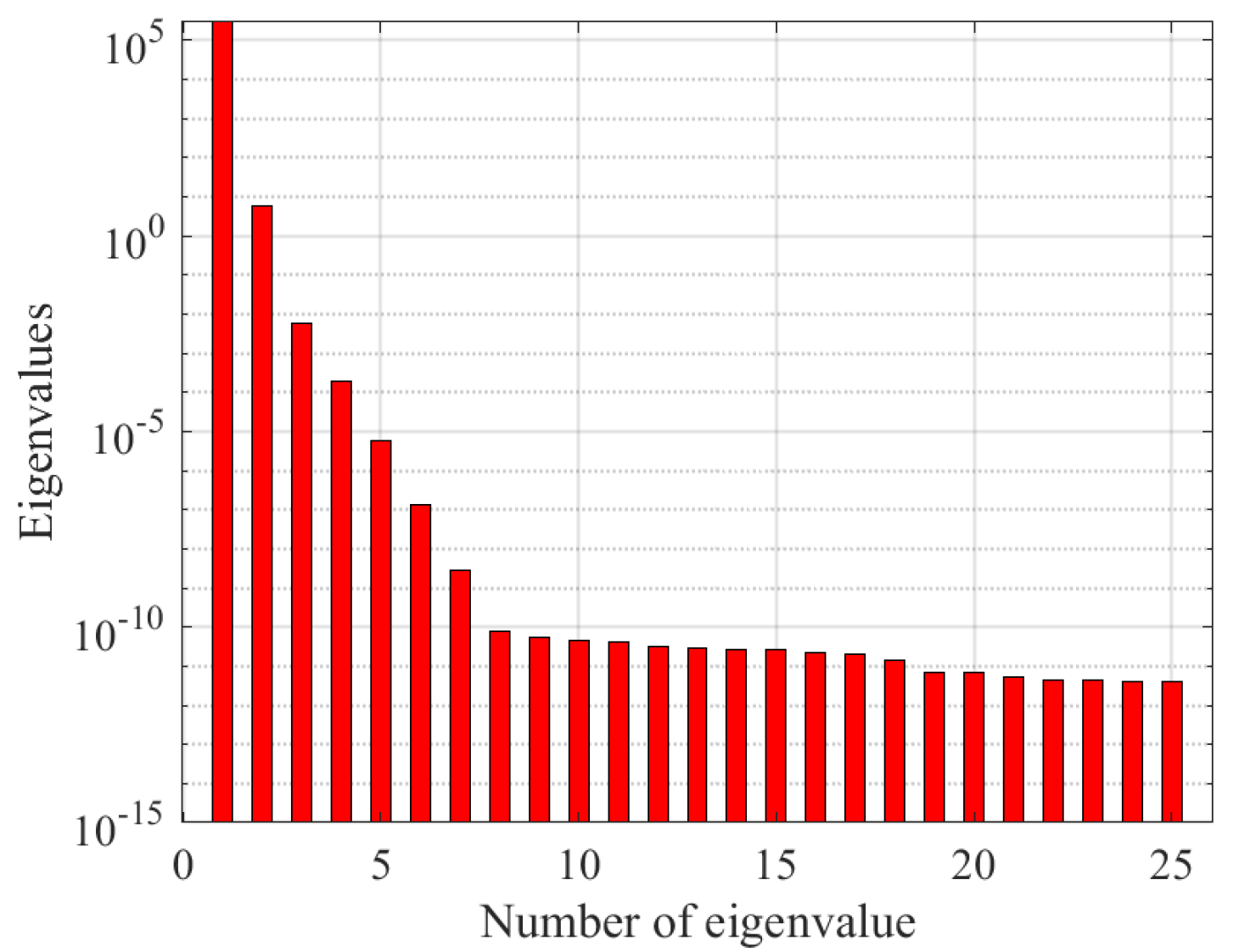
In this example, for the purpose of comparison, three types of meshes are considered, that is, $10\times 10$, $20\times 20$ and $40\times 40$ square elements. For all tests in the example, the time-step $\mathsf{\Delta }t=0.001$ and calculate until $t=1$, and the snapshots are generated by the FEM. The eigenvalues of the snapshot matrix for $20\times 20$ square elements are shown in Figure 1. From the computed results, we can distinctly find these eigenvalues decay rapidly and the first eigenvalue accounts for more than 99% of the accumulated energy. As we will soon see, the number of POD basis r from 1 to 6 can give the satisfactory numerical results for this example.

Table 1. Comparison of computational times (s) for Example 1, utilizing $\mathsf{\Delta }t=0.001,\tau =0.1$, and varying numbers of elements and POD bases.

Elements	$\mathit{r}=3$		$\mathit{r}=6$
	FEM	FEM-POD	FEM	FEM-POD
$10\times 10$	0.140216	0.056844	0.140133	0.055176
$20\times 20$	0.880241	0.078657	0.915028	0.078721
$40\times 40$	4.508071	0.110092	4.520868	0.111787

shows the FEM and FEM-POD calculation times for different meshes and r with $\mathsf{\Delta }t=0.001$. As the number of elements increases, the effect of POD in reducing the calculation time becomes more obvious. Meanwhile, when the number of POD basis r is changed from 3 to 6, the computational time of FEM-POD almost unchanged in the same elements and considering the systematic error of computer timing.

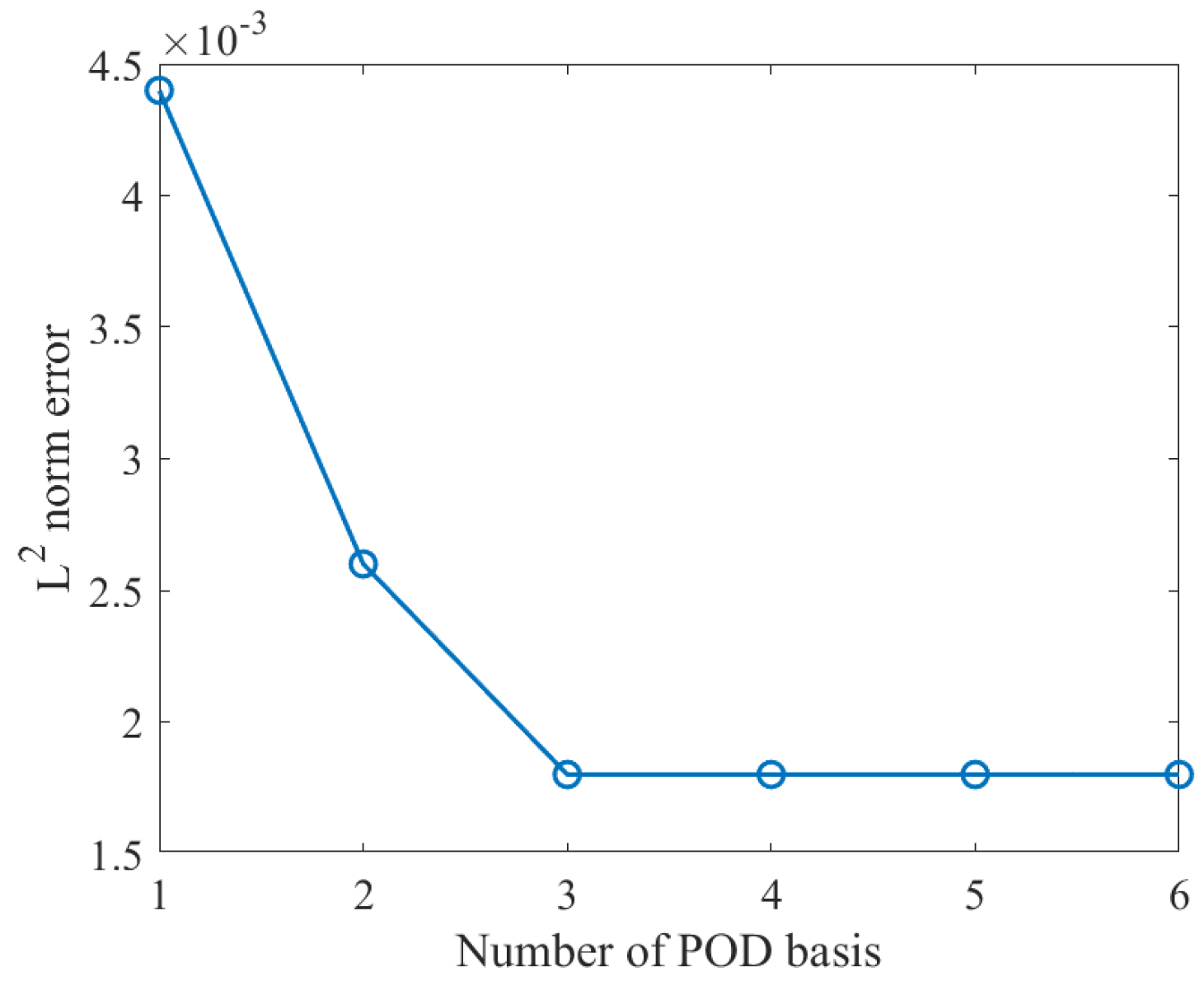
Figure 2 illustrates the correlation between the quantity of POD bases and the $L^2$ norm error when $\mathsf{\Delta }t=0.001$ and using $20\times 20$ square elements at $t=1$. Evidently, a limited number of POD bases suffice to minimize the $L^2$ norm error, highlighting the FEM-POD’s efficiency in significantly diminishing unknown variables while maintaining satisfactory computational precision. Furthermore, as the number of POD bases r increases beyond a certain threshold, the $L^2$ norm error plateaus. 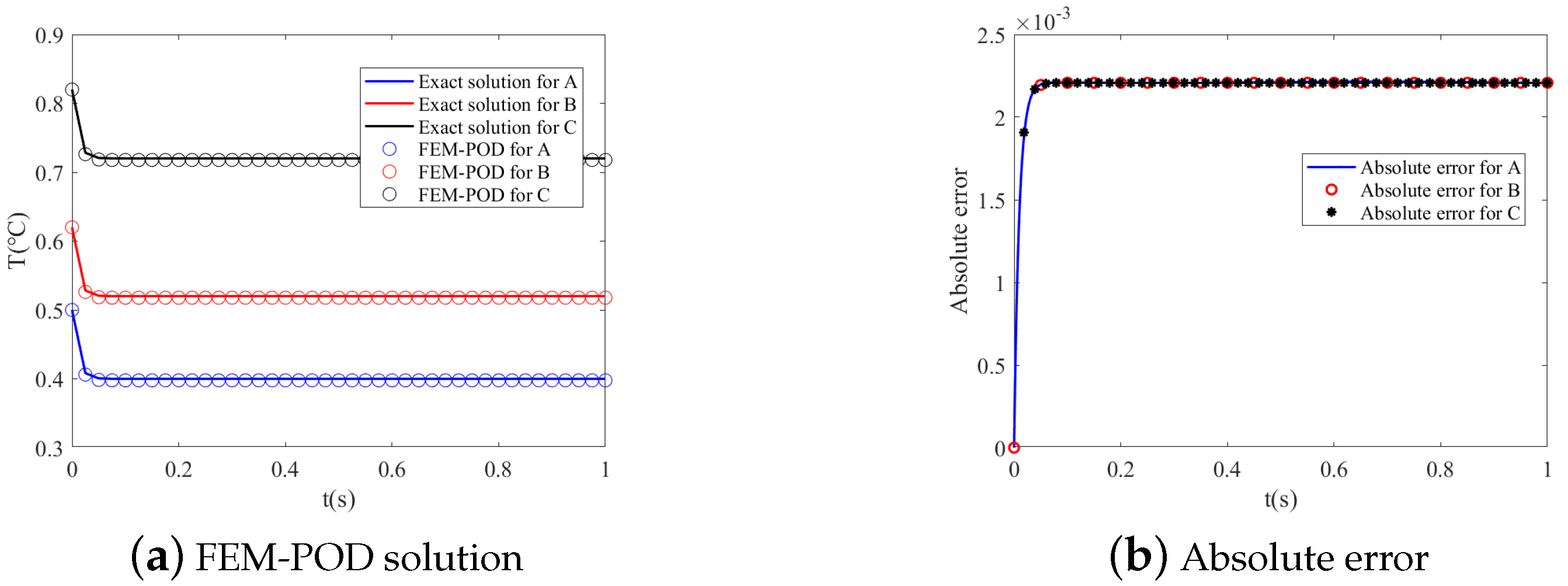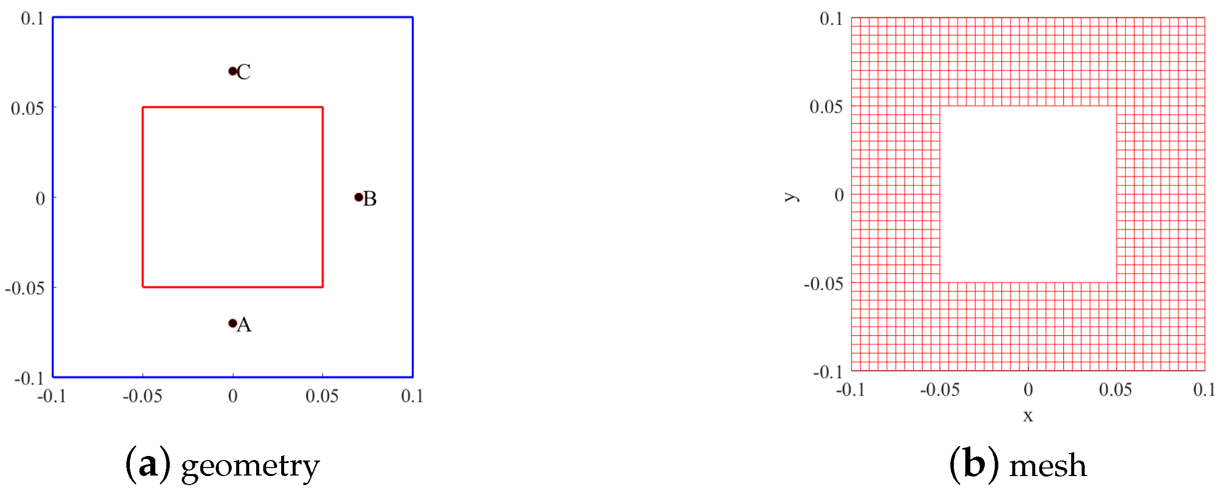Additionally, Figure 3 compares the numerical solutions at points A$(0.6,0.2)$, B$(0.6,0.4)$ and C$(0.6,0.6)$ between the FEM-POD approach and the exact solution, revealing excellent alignment between the two sets of results.

• Example 2

We consider a rectangular domain $\mathsf{\Omega }=[0,5]\times [0,0.5]$ subjected to various types of laser heat sources. In this scenario, the heat conductivity is set to $k=1 \mathrm{W}/(\mathrm{m}·°\mathrm{C})$, and the heat capacity ratio is $\rho c=2 \mathrm{J}/({\mathrm{m}}^3·°\mathrm{C})$. The initial condition for this example is provided as follows

$$\left\{\begin{array}{c}\theta (\mathit{x},0)=0,\hfill \\ \frac{\partial \theta (\mathit{x},0)}{\partial t}=2exp(-x).\hfill \end{array}\right.$$

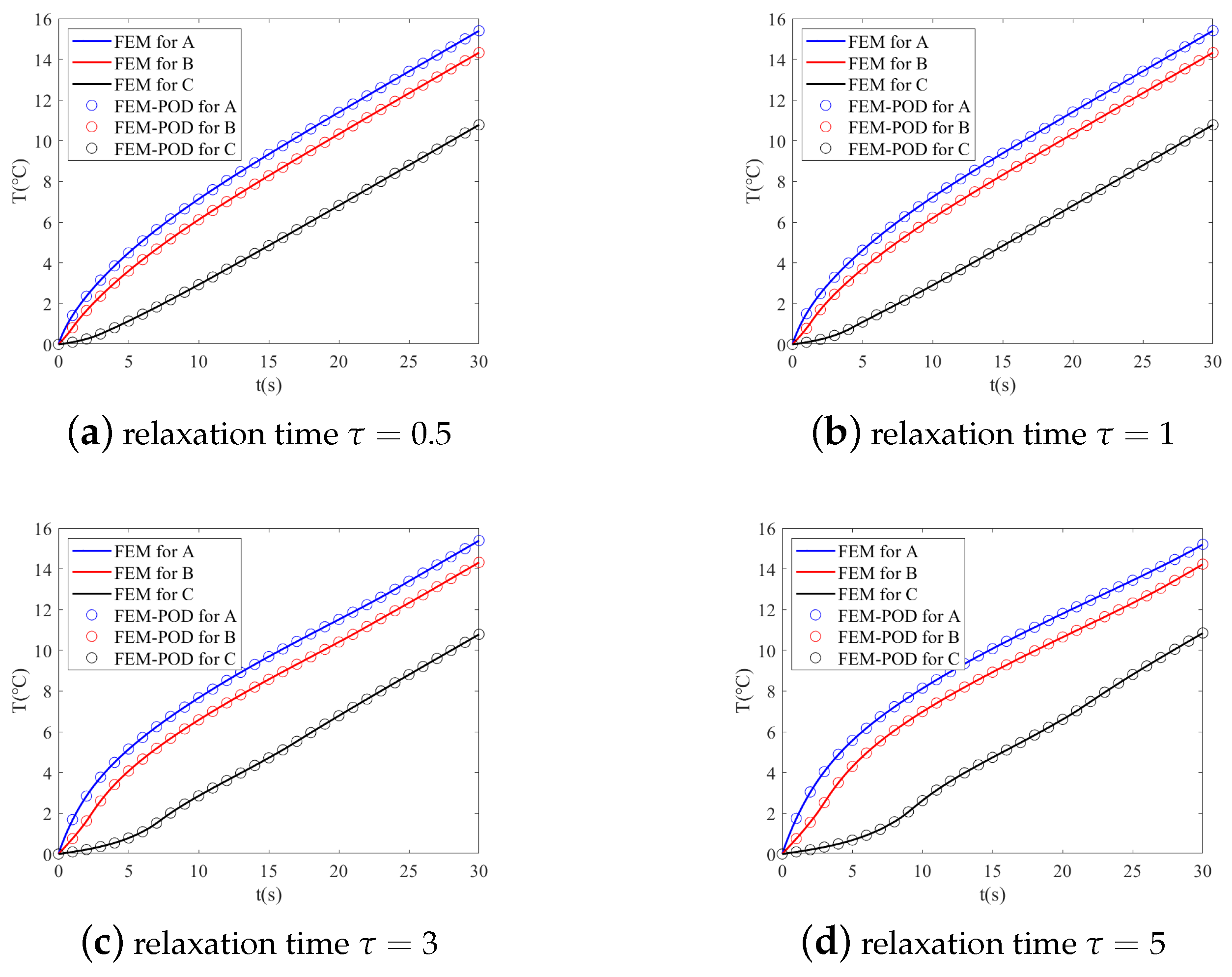
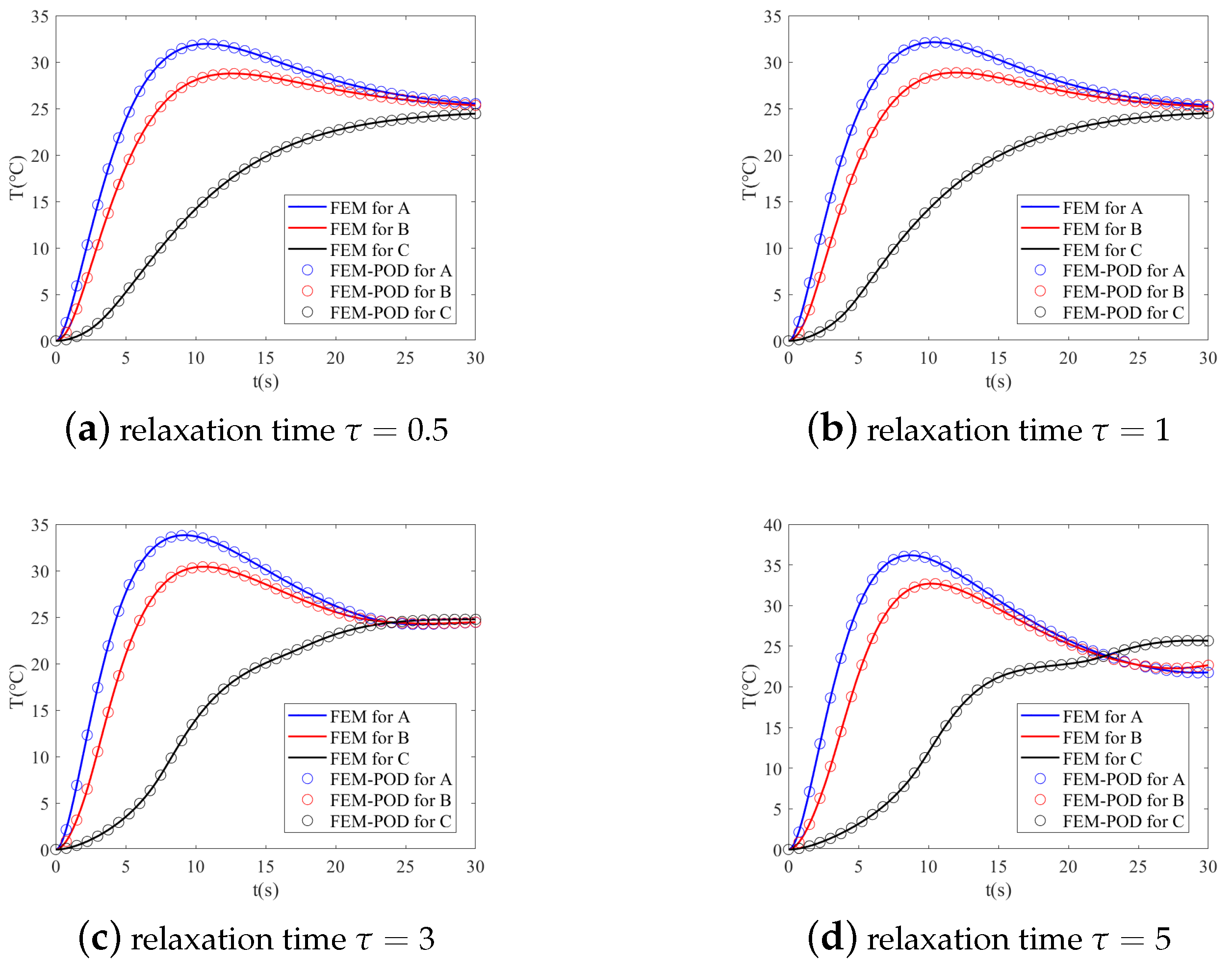
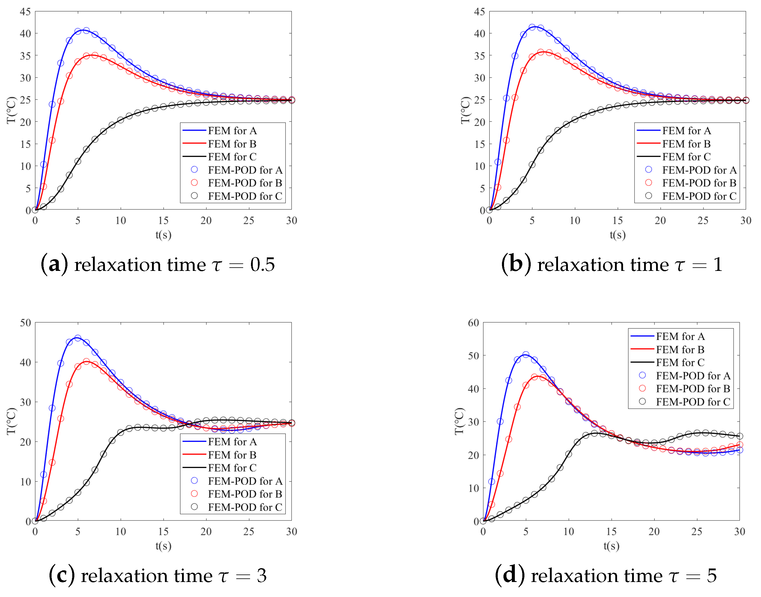
When $t>0$, the boundary of the rectangular domain is adiabatic. In the example, we consider the four different relaxation time $\tau =0.5$ s, 1 s, 3 s, 5 s and the following three types of laser heat source:

Case 1. The time-independent laser heat source with a constant intensity distribution: $Q(\mathit{x},t)=4exp(-x)$.

Case 2. The time-dependent laser heat source applied at specific locations within the domain: $Q(\mathit{x},t)=100[exp(-0.2t)-exp(-0.4t\left)\right]exp(-x)$.

Case 3. The time-dependent laser heat source applied at specific locations within the domain: $Q(\mathit{x},t)=200[exp(-0.4t)-exp(-0.8t\left)\right]exp(-x)$.

For the purpose of comparison, in this example, three kinds of meshes are used, that is, $25\times 10, 50\times 20$, and $100\times 40$ rectangular elements. In fact, there is currently no analytical solution to the problem, but we also use the solution given in ref. [25] as the reference solution of the problem, just like Yao et al. [8]. 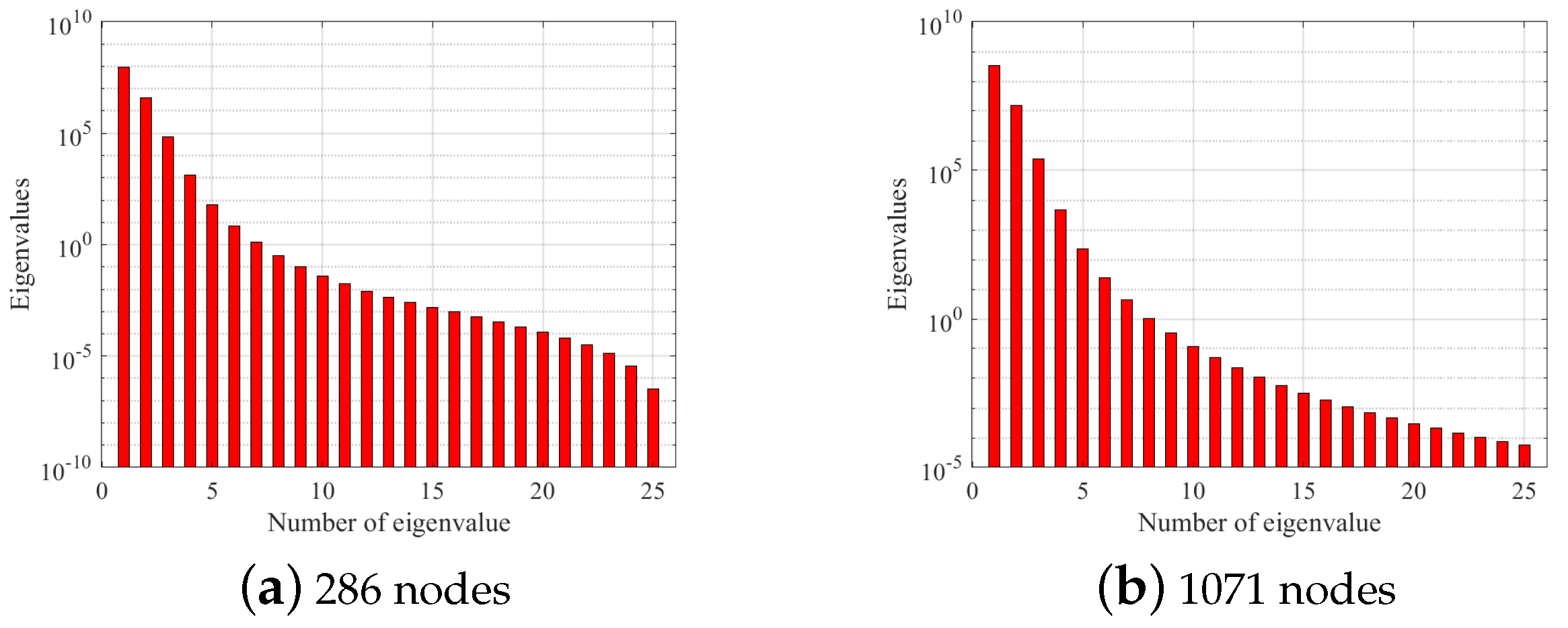For all tests in the example, we take the time step $\mathsf{\Delta }t=0.01$ and the snapshots are generated by FEM. The first 25 eigenvalues of the snapshots matrix for $25\times 10$ elements and $50\times 20$ elements are shown in Figure 4. From the numerical point of view, the size of the eigenvalues drop very quickly, and the accumulation of the first three eigenvalues accounts for more than 99% of all the eigenvalues. Thus, we take $r=10$ in this example for all the nodal distribution, that is, we only need 10 POD basis.

Table 2. Temperatures of nodes along the line $y=0.25$ with $\mathsf{\Delta }t=0.01,\tau =0.5,r=10$ for Case 1 of Example 2.

x	$\mathit{t}=0.5$			$\mathit{t}=1.0$
	FEM	FEM-POD	Exact [8]	FEM	FEM-POD	Exact [8]
0.0	0.8154	0.8160	0.8144	1.4167	1.4196	1.4156
0.5	0.6292	0.6293	0.6268	1.2127	1.2150	1.2119
1.0	0.3800	0.3802	0.3802	0.8204	0.8199	0.8187
1.5	0.2305	0.2298	0.2306	0.4963	0.4957	0.4966
2.0	0.1398	0.1404	0.1399	0.3010	0.3013	0.3012
2.5	0.0848	0.0845	0.0848	0.1826	0.1825	0.1827

and

Table 3. Temperatures of nodes along the line $y=0.25$ with $\mathsf{\Delta }t=0.01,\tau =0.5,r=10$ for Case 2 of Example 2.

x	$\mathit{t}=0.5$			$\mathit{t}=1.0$
	FEM	FEM-POD	Exact [8]	FEM	FEM-POD	Exact [8]
0.0	0.9736	0.9758	0.9784	3.1640	3.1610	3.1687
0.5	0.6943	0.6944	0.6990	2.5391	2.5405	2.5440
1.0	0.4206	0.4212	0.4240	1.6040	1.6041	1.6090
1.5	0.2551	0.2545	0.2571	0.9722	0.9723	0.9759
2.0	0.1547	0.1548	0.1560	0.5897	0.5901	0.5919
2.5	0.0938	0.0945	0.0946	0.3577	0.3568	0.3590

show the comparison of the results obtained by FEM, FEM-POD and the reference solution taken from [8]. The results demonstrate that the FEM-POD solutions are in good agreement with both the reference solution and the FEM solutions, regardless of whether a time-independent or time-dependent laser heat source is used. This indicates that FEM-POD has a high level of computational accuracy for non-Fourier heat conduction problems. To assess the computational accuracy of FEM-POD, Figure 5, Figure 6 and Figure 7 compare the computed temperature histories at point A$(0,0.25)$, point B$(1.0,0.25)$ and point C$(3.0,0.25)$ using FEM-POD and FEM with varying relaxation times and laser heat sources. It is clear from these figures that, at first glance, the present numerical solutions are very close to the FEM solutions under the different relaxation time and laser heat source. 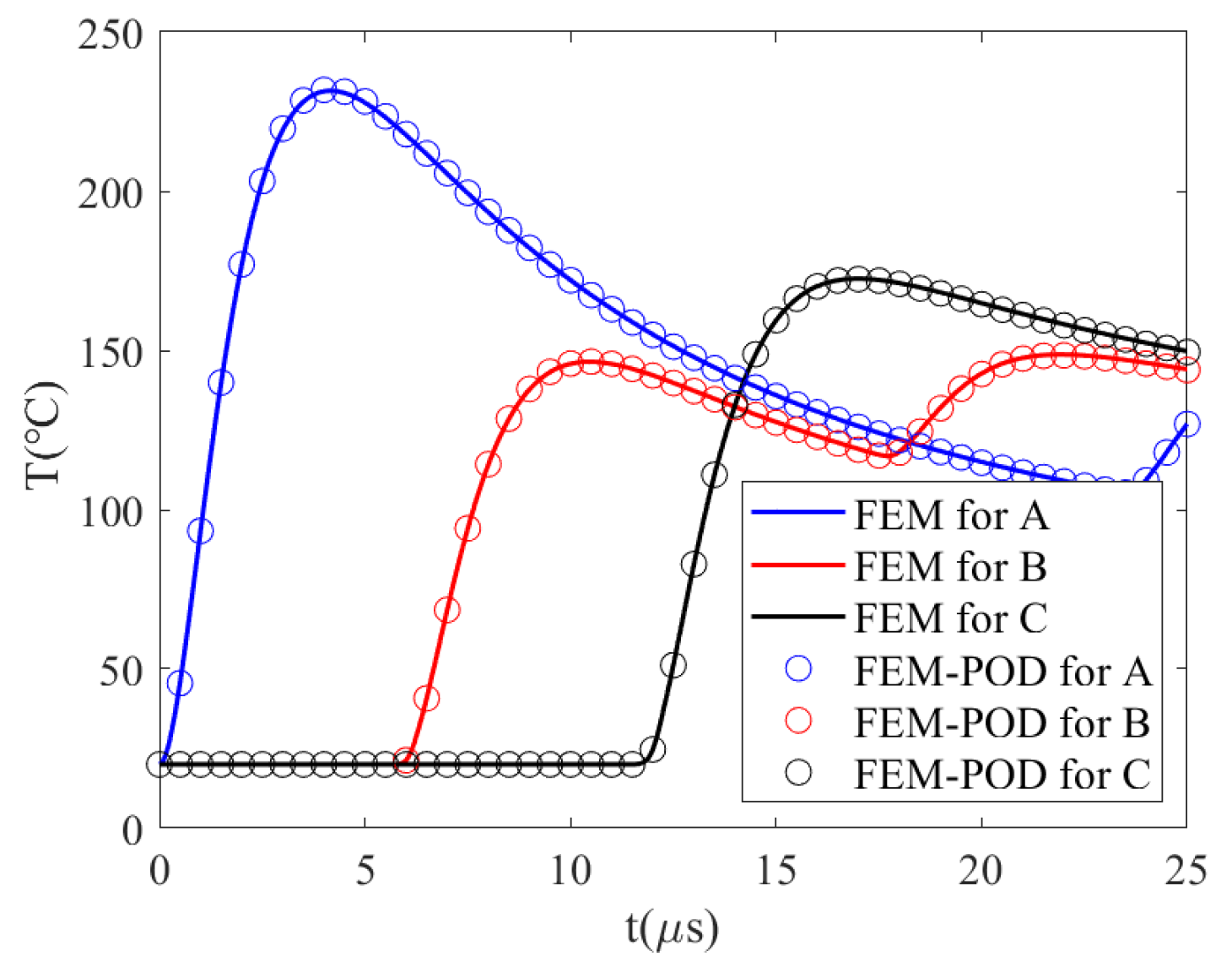For the time-independent laser heat source, the temperatures at the three points increase with time as shown in Figure 5 for all considered relaxation time. For the time-dependent laser heat source, the temperatures at points A and B increase rapidly with time and reach a maximum value, and then decreased slowly. However, the temperatures at point C generally increase with time for four different relaxation times.

Table 4. Comparison of the computational time(s) for Example 2 with $\mathsf{\Delta }t=0.01,\tau =0.5,r=10$.

Nodes	FEM	FEM-POD
286	0.136045	0.029175
1071	0.714073	0.042831
4141	7.549349	0.127767

illustrates the computational times of both FEM and FEM-POD across different nodal distributions, utilizing parameters of $\mathsf{\Delta }t=0.01,\tau =0.5$, and $r=10$ at $t=30$ s. It is evident that, for identical node distributions, FEM-POD consistently demonstrates a reduced computational time compared to FEM. Furthermore, as the number of nodes increases, the computational time saved by FEM-POD becomes more pronounced in comparison to FEM, highlighting its effectiveness in enhancing computational efficiency.

• Example 3

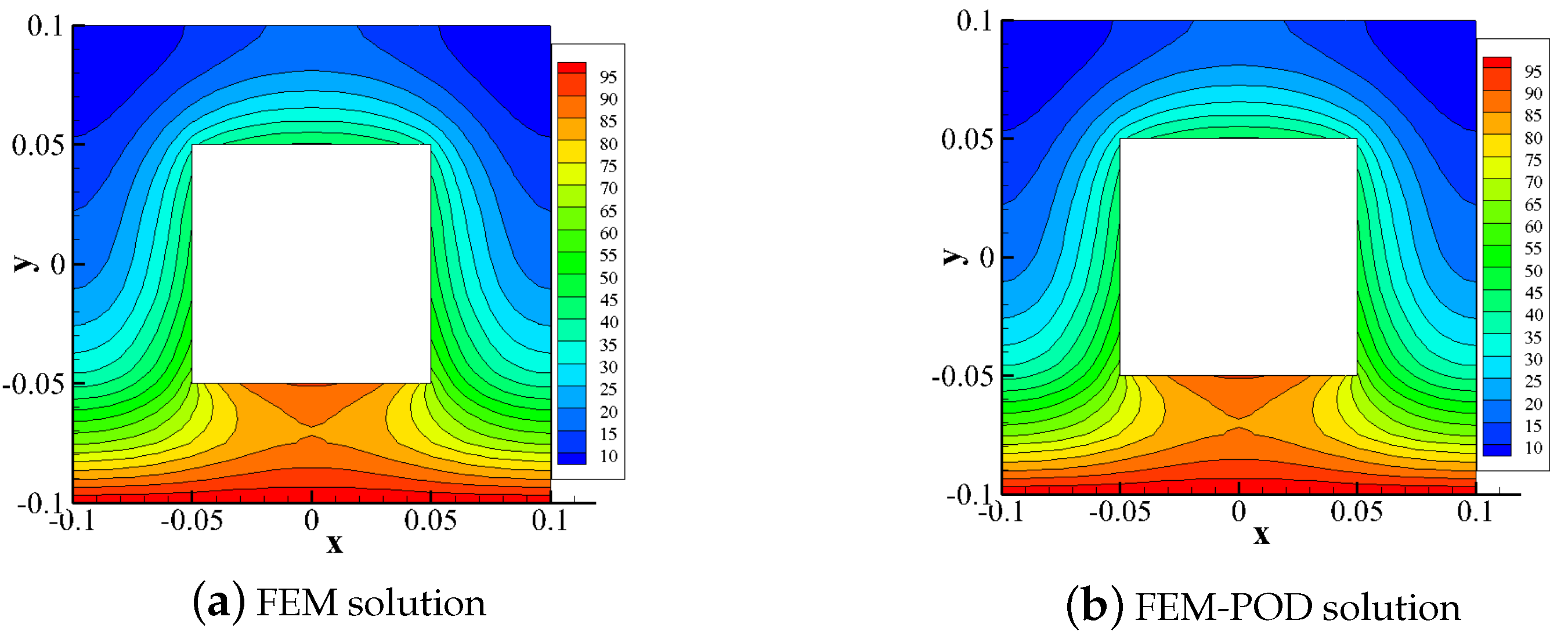
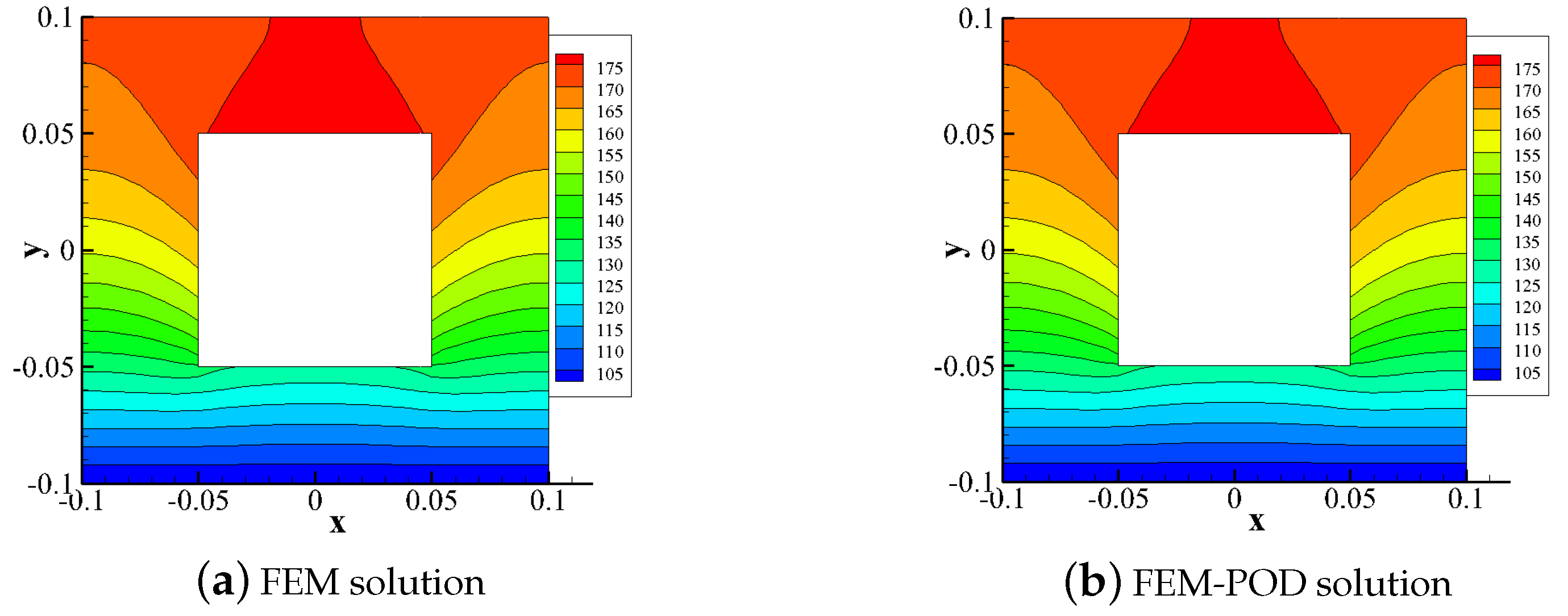
In this example, we consider a large square domain denoted by ${\mathsf{\Omega }}_1={[-0.1,0.1]}^2$ which contains a smaller square hole represented by ${\mathsf{\Omega }}_2={[-0.05,0.05]}^2$ as depicted in Figure 8a. The material properties within this domain are characterized by a heat conductivity of $k=130 \mathrm{W}/(\mathrm{m}·°\mathrm{C})$, a heat capacity of $c=400 \mathrm{J}/(\mathrm{K}\mathrm{g}·°\mathrm{C})$, and a density of $\rho =2700 \mathrm{K}\mathrm{g}/{\mathrm{m}}^3$. Additionally, a relaxation time of $\tau =0.5$ s is specified. The initial conditions are set to 0 °C throughout the domain. The outer lower boundary is maintained at a temperature of 100 °C while the Robin boundary conditions are applied to the remaining boundaries. These Robin conditions involve a heat transfer coefficient of $h=1000 \mathrm{W}/({\mathrm{m}}^2·°\mathrm{C})$ and an ambient temperature of 200 °C. As in the previous examples, here we consider three kinds of meshes, namely 300 elements, 1200 elements (as shown in Figure 8b) and 7500 elements. Meanwhile, the time step $\mathsf{\Delta }t=1\mathrm{s}$ and the end time is 250 s.

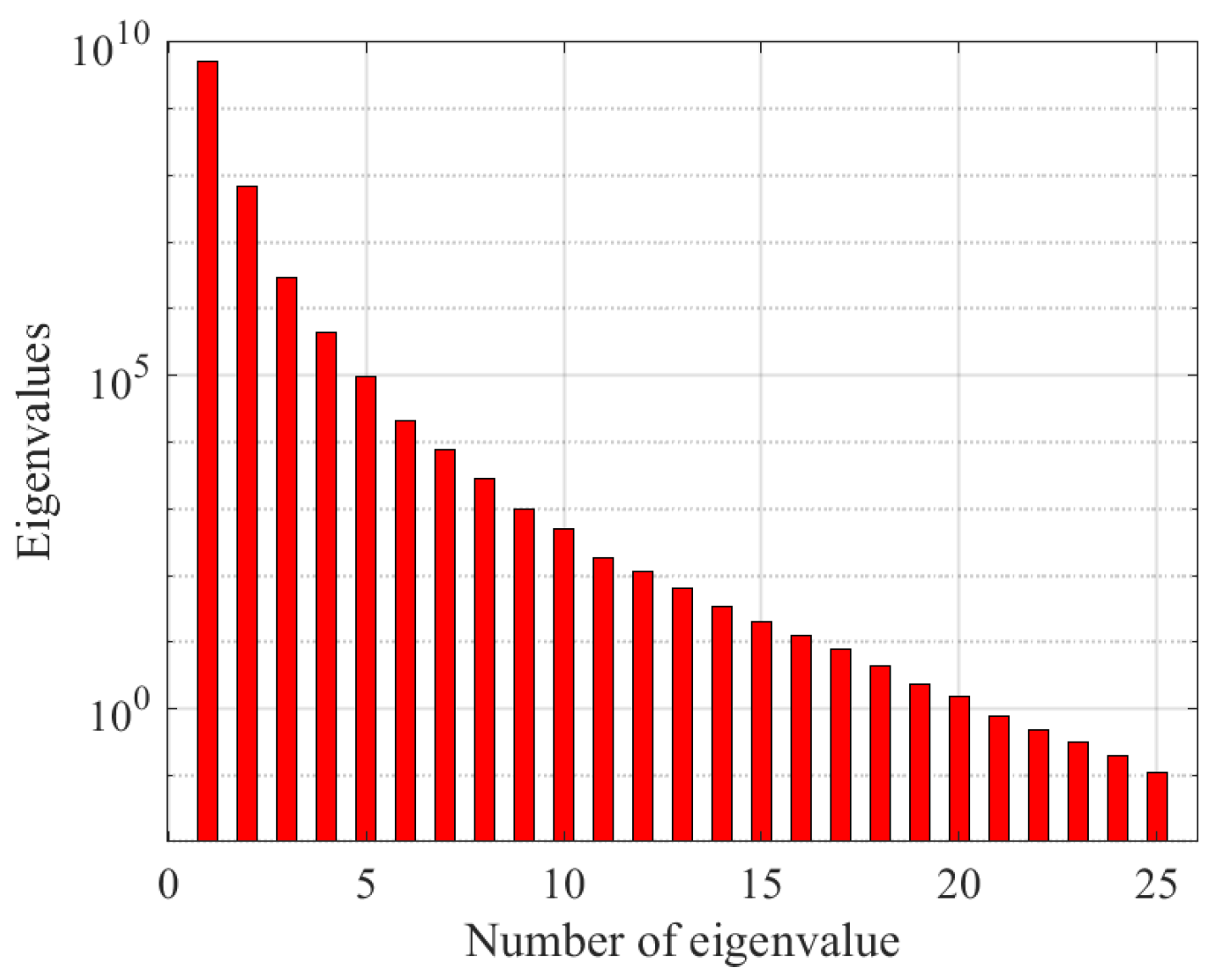
Figure 9 illustrates the eigenvalues for an example comprising 1320 nodes and 1200 elements. Notably, these eigenvalues exhibit a rapid decay pattern. Through these computational results, using Equation (21), when we take $r=12$, the accumulating energy of the whole eigenvalue information will reach 99.99%. Thus, we take 12 POD basis for this example with all meshes. Figure 10 and Figure 11 depict the temperature contours obtained using both FEM and FEM-POD at time instances $t=10$ s and $t=250$ s, respectively, with 1320 nodes. Upon visual inspection of these figures, it is evident that the temperature distributions computed by FEM-POD exhibit strong agreement with those generated by the FEM. 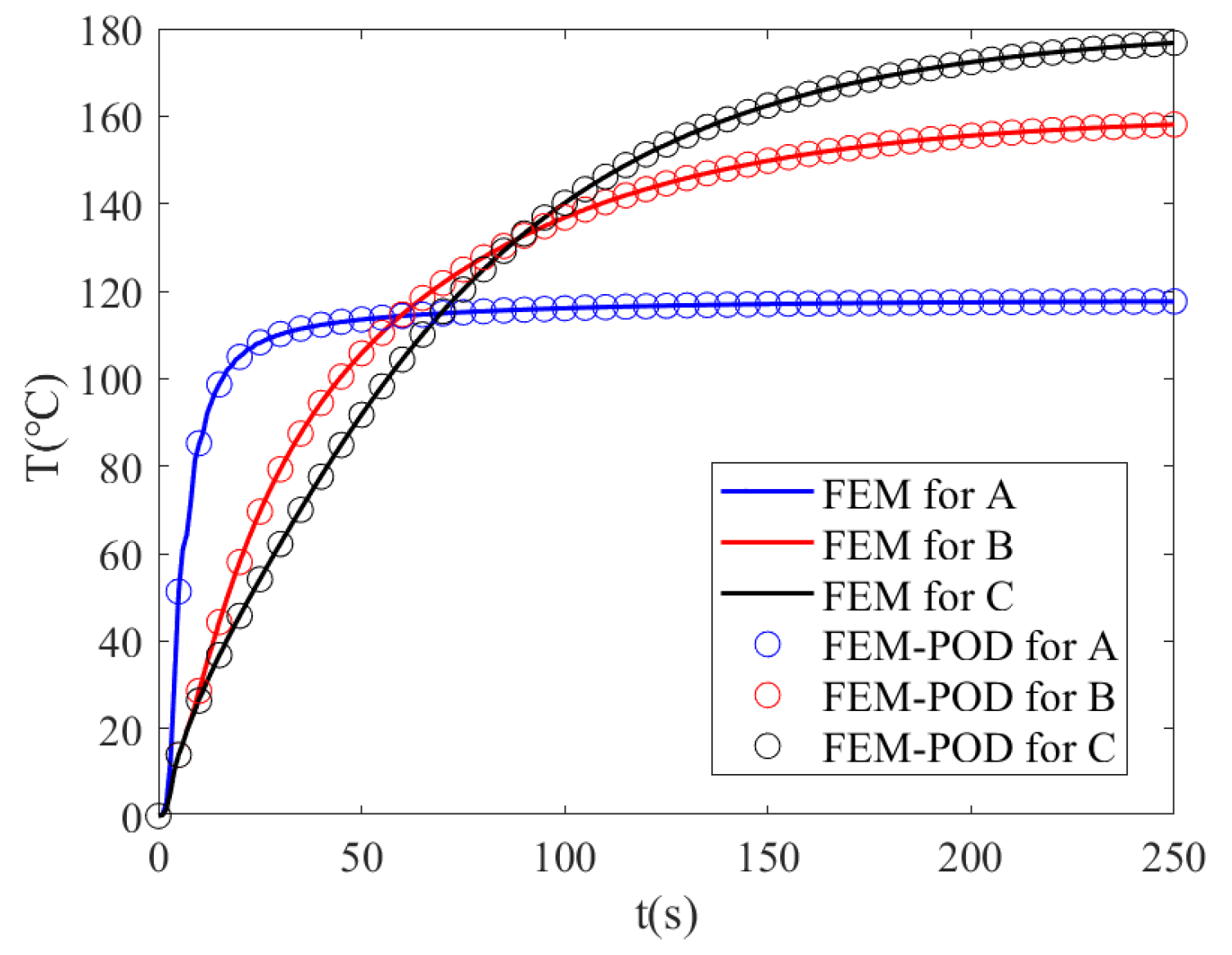To further substantiate the computational accuracy of FEM-POD, a comparative analysis is presented in Figure 12, which compares the temperature histories at points A$(0,-0.07)$, point B$(0.07,0)$ and point C$(0,0.07)$ obtained from both methods. As we expected, the temperatures at three points obtained by FEM-POD matched those obtained by FEM very well.

Table 5. Comparison of the computational time(s) for Example 3 with $\mathsf{\Delta }t=1,\tau =0.5,r=12$.

Nodes	Elements	FEM	FEM-POD
360	300	0.038014	0.016318
1320	1200	0.219562	0.028162
7800	7500	3.218023	0.109611

presents a comparison of the computational times between FEM and FEM-POD for Example 3, with parameters set to $\mathsf{\Delta }t=1,\tau =0.5,r=12$ across varying numbers of nodes. The data unequivocally demonstrates that FEM-POD offers significant computational savings compared to the traditional FEM when addressing non-Fourier heat conduction problems. This advantage becomes increasingly apparent as the number of nodes and elements increases. This example reinforces the fact that FEM-POD not only maintains computational accuracy but also significantly enhances computational efficiency compared to the FEM. Consequently, the proposed FEM-POD method is highly suitable for rapidly solving non-Fourier heat conduction problems.

• Example 4

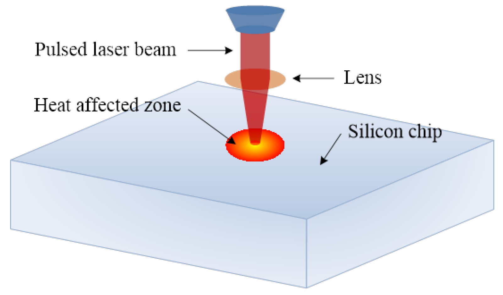
In this example, we consider the following three-dimensional model, that is, a silicon chip with sizes of $5\mathrm{m}\mathrm{m}\times 5\mathrm{m}\mathrm{m}\times 50\mathsf{\mu }\mathrm{m}$ (for length, width and thickness, respectively) is considered as shown in Figure 13. The material properties of the chip include a heat conductivity of $k=148 \mathrm{W}/(\mathrm{m}·°\mathrm{C})$, a heat capacity of $c=700 \mathrm{J}/(\mathrm{K}\mathrm{g}·°\mathrm{C})$, a density of $\rho =2330\mathrm{K}\mathrm{g}/{\mathrm{m}}^3$, and a relaxation time of $\tau =5\mathsf{\mu }s$. The initial conditions for the chip are set at a uniform temperature of 20 °C, and all surfaces are assumed to be thermally insulated. A transient pulse laser is then applied to a portion of the center of the top surface, introducing a heating source represented by $Q(\mathit{x},t)={10}^{16}texp(-{10}^{6}t)$. 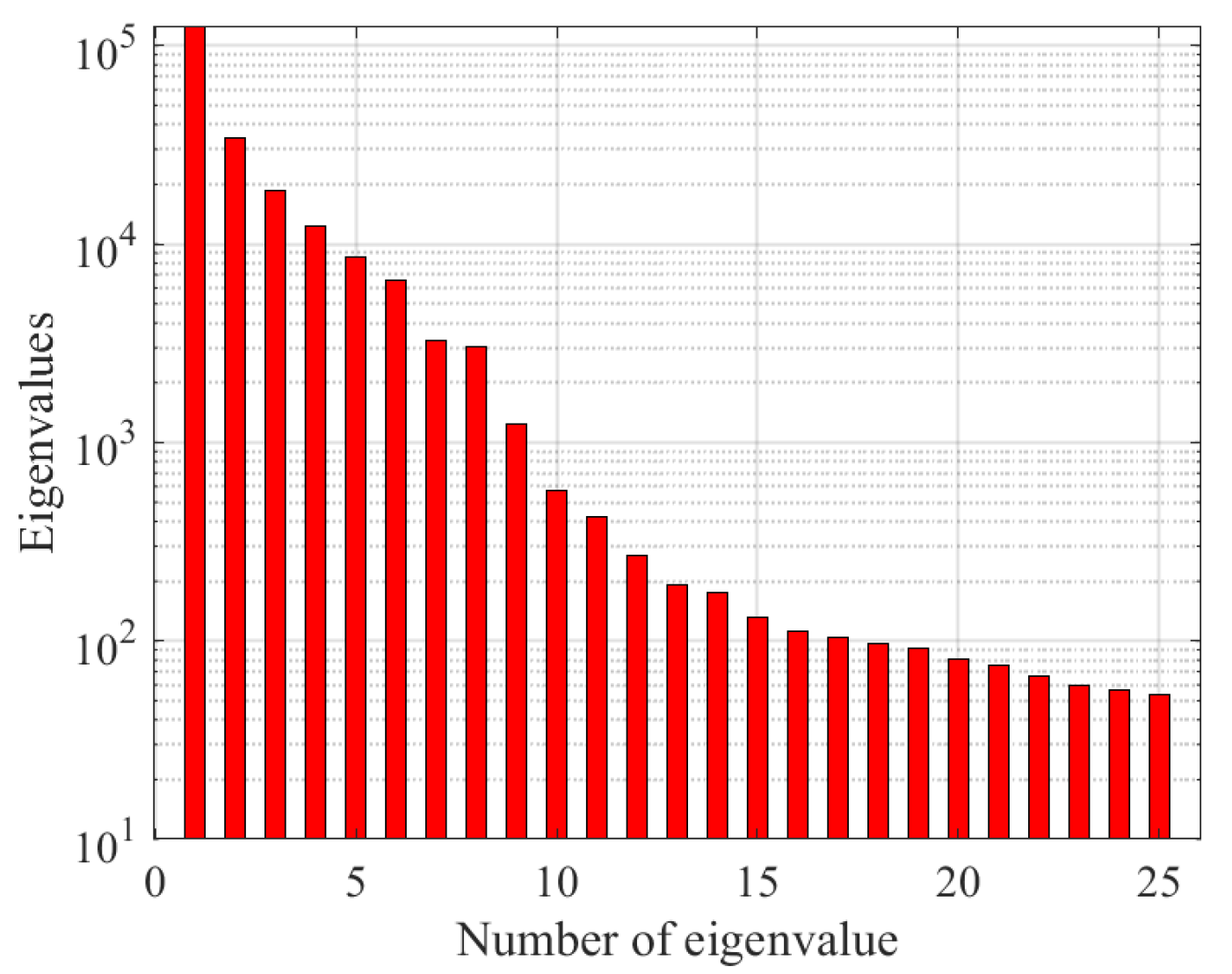Figure 14 presents a plot of the eigenvalues computed for this three-dimensional problem using 32,000 hexahedral elements. The plot reveals that the eigenvalues decrease monotonically, indicating a reduction in the system’s thermal response over time. However, it is worth noting that the rate of decline in the eigenvalues is not as pronounced as it was in the two-dimensional case, suggesting a more gradual dissipation of heat energy in the three-dimensional model. 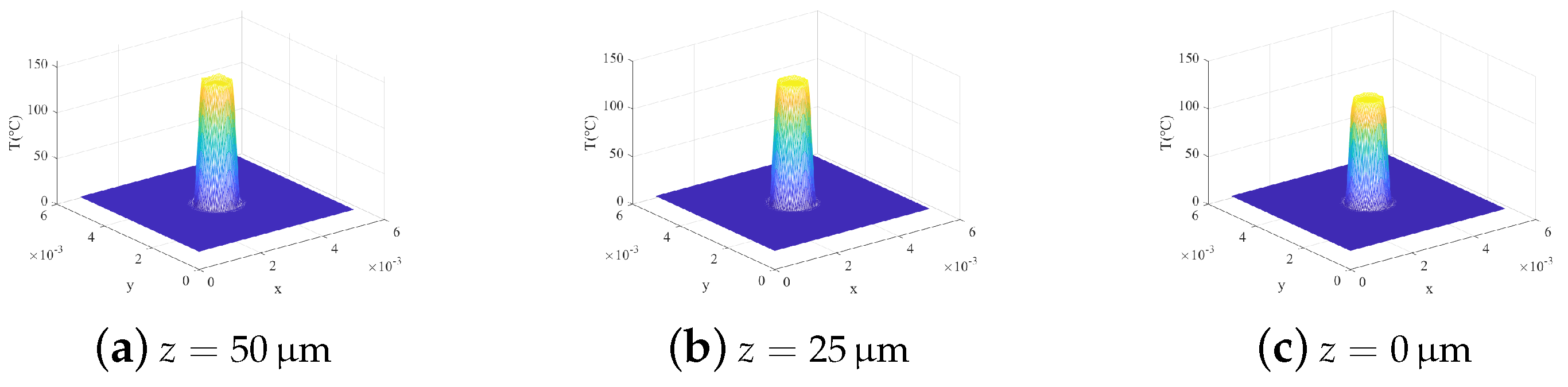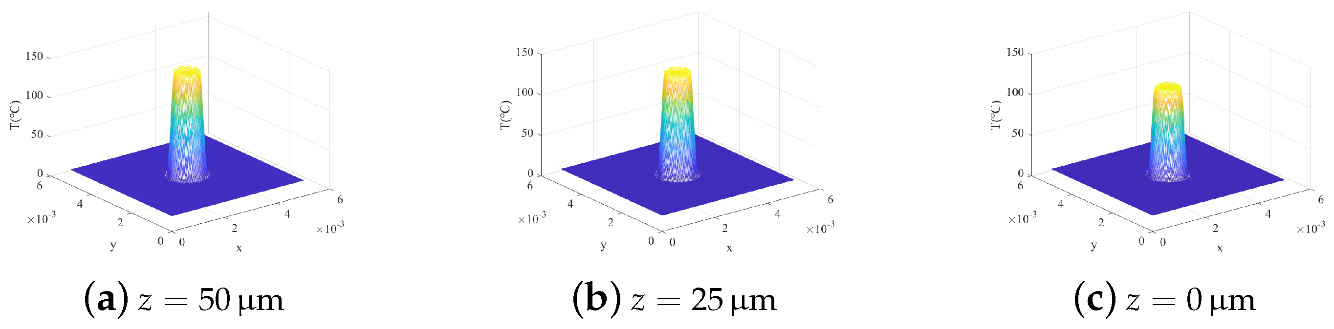Figure 15 and Figure 16 show the temperature distributions of FEM and FEM-POD at time $t=25\mathsf{\mu }\mathrm{s}$ with 32,000 hexahedral elements along the top surface, center layer and bottom surface of the silicon chip. It can be found that the solutions obtained by FEM and FEM-POD are identical with each other. Similar to Example 3, we present a detailed comparison of the computational results obtained using both the Finite Element Method (FEM) and the Finite Element Method enhanced with Proper Orthogonal Decomposition (FEM-POD) as shown in Figure 17. Specifically, we focus on the temperature histories at three critical points within the silicon chip: Point A$(2.5\mathrm{m}\mathrm{m},2.5\mathrm{m}\mathrm{m},50\mathsf{\mu }\mathrm{m})$, point B$(2.5\mathrm{m}\mathrm{m},2.5\mathrm{m}\mathrm{m},25\mathsf{\mu }\mathrm{m})$ and point C$(2.5\mathrm{m}\mathrm{m},2.5\mathrm{m}\mathrm{m},0\mathsf{\mu }\mathrm{m})$. As expected, the temperatures calculated at these points using the FEM-POD technique align closely with those determined through the traditional FEM approach. This confirms the accuracy of the FEM-POD method in simulating the thermal behavior of the chip. To further evaluate the computational efficiency of both methods, we compared their CPU running times. These simulations were performed using a time step of $\mathsf{\Delta }t=5\times {10}^{-2}\mathsf{\mu }$s and a relaxation time of $\tau =5\mathsf{\mu }$s, while varying the number of elements. For this analysis, we utilized 20 POD bases ($r=20$) (

Table 6. Comparison of the computational time(s) for Example 4 with $\mathsf{\Delta }t=5\times {10}^{-2}\mathsf{\mu }\mathrm{s},\tau =5\mathsf{\mu }$s, $r=20$.

Elements	FEM	FEM-POD
$300\times 300\times 15$	1026.97	6.542
$160\times 1600\times 8$	271.66	1.235
$80\times 80\times 5$	42.98	0.3648
$40\times 40\times 3$	8.16	0.1721

). The results clearly demonstrate that the CPU running time required for the FEM-POD simulations is significantly less than that of the full-order FEM simulations. This substantial reduction in computational time highlights the practical advantages of incorporating the POD technique into FEM-based simulations, particularly for complex three-dimensional models where computational efficiency is crucial.

5. Conclusions

This study successfully introduces a model reduction technique known as FEM-POD, which combines the FEM with the POD and utilizes the Newmark scheme for temporal discretization. This innovative approach effectively addresses non-Fourier heat conduction problems. The numerical results presented for four distinct examples consistently illustrate that the FEM-POD method significantly outperforms the traditional FEM method in terms of prediction time, while maintaining equivalent computational accuracy. Notably, although the primary emphasis of this paper is on the integration of FEM and POD, the underlying principles of the FEM-POD methodology can be seamlessly applied to other numerical techniques, including the Boundary Element Method (BEM) or Meshless methods.

References

1. Wang, L.; Xu, J.; Wang, J. A peridynamic framework and simulation of non-Fourier and nonlocal heat conduction. Int. J. Heat Mass Transf. 2018, 118, 1284–1292. [Google Scholar] [CrossRef]
2. Aznam, S.M.; Chowdhury, M. Generalized Haar wavelet operational matrix method for solving hyperbolic heat conduction in thin surface layers. Results Phys. 2018, 11, 243–252. [Google Scholar] [CrossRef]
3. Majchrzak, E.; Mochnacki, B. Application of numerical methods for solving the non-fourier equations. A review of our own and collaborators’ works. J. Appl. Math. Comput. Mech. 2018, 17, 43–53. [Google Scholar] [CrossRef]
4. Xu, B.; Li, B. Finite element solution of non-Fourier thermal wave problems. Numer. Heat Transf. Part B Fundam. 2003, 44, 45–60. [Google Scholar] [CrossRef]
5. Wang, B.L.; Han, J.C. A finite element method for non-Fourier heat conduction in strong thermal shock environments. Front. Mater. Sci. China 2010, 4, 226–233. [Google Scholar] [CrossRef]
6. Yuvaraj, R.; Senthil Kumar, D. Numerical simulation of thermal wave propagation and collision in thin film using finite element solution. J. Therm. Anal. Calorim. 2020, 142, 2351–2369. [Google Scholar] [CrossRef]
7. Han, S.; Peddieson, J. Non-Fourier heat conduction/convection in moving medium. Int. J. Therm. Sci. 2018, 130, 128–139. [Google Scholar] [CrossRef]
8. Yao, W.A.; Yao, H.X.; Yu, B. Radial integration BEM for solving non-Fourier heat conduction problems. Eng. Anal. Bound. Elem. 2015, 60, 18–26. [Google Scholar] [CrossRef]
9. Yu, B.; Yao, W.A.; Zhou, H.L.; Chen, H.L. Precise time-domain expanding BEM for solving non-Fourier heat conduction problems. Numer. Heat Transf. Part B Fundam. 2015, 68, 511–532. [Google Scholar] [CrossRef]
10. Vishwakarma, V.; Das, A.K.; Das, P. Analysis of non-Fourier heat conduction using smoothed particle hydrodynamics. Appl. Therm. Eng. 2011, 31, 2963–2970. [Google Scholar] [CrossRef]
11. Khosravifard, A.; Hematiyan, M.R. Meshless analysis of casting process considering non-Fourier heat transfer. Iran. J. Mater. Form. 2016, 3, 13–25. [Google Scholar]
12. Wen, Z.; Hou, C.; Zhao, M.; Wan, X. A peridynamic model for non-Fourier heat transfer in orthotropic plate with uninsulated cracks. Appl. Math. Model. 2023, 115, 706–723. [Google Scholar] [CrossRef]
13. Liu, Y.; Li, L. Lattice Boltzmann simulation of non-Fourier heat conduction with phase change. Numer. Heat Transf. Part A Appl. 2019, 76, 19–31. [Google Scholar] [CrossRef]
14. Liu, Y.; Li, L.; Zhang, Y. Numerical simulation of non-Fourier heat conduction in fins by lattice Boltzmann method. Appl. Therm. Eng. 2020, 166, 114670. [Google Scholar] [CrossRef]
15. Huang, M.; Tang, J.; Zhao, Y.; Ouyang, X. A new efficient and accurate procedure for solving heat condution problems. Int. J. Heat Mass Transf. 2017, 111, 508–519. [Google Scholar] [CrossRef]
16. Zhang, X.; Xiang, H. A fast meshless method based on proper orthogonal decomposition for the transient heat conduction problems. Int. J. Heat Mass Transf. 2015, 84, 729–739. [Google Scholar] [CrossRef]
17. Luo, Z.; Chen, G. Proper Orthogonal Decomposition Methods for Partial Differential Equations; Academic Press: London, UK, 2019. [Google Scholar]
18. Zhao, J.; Rui, H.; Song, J. A reduced-order Weak Galerkin finite element algorithm based on POD technique for parabolic problem on polytopal mesh. Appl. Math. Lett. 2022, 127, 107842. [Google Scholar] [CrossRef]
19. Eroglu, F.G.; Kaya, S.; Rebholz, L.G. A modular regularized variational multiscale proper orthogonal decomposition for incompressible flows. Comput. Methods Appl. Mech. Eng. 2017, 325, 350–368. [Google Scholar] [CrossRef]
20. Zhang, X.; Zhang, P. A reduced high-order compact finite difference scheme based on proper orthogonal decomposition technique for KdV equation. Appl. Math. Comput. 2018, 339, 535–545. [Google Scholar] [CrossRef]
21. Luo, Z.; Li, H.; Sun, P. A reduced-order Crank–Nicolson finite volume element formulation based on POD method for parabolic equations. Appl. Math. Comput. 2013, 219, 5887–5900. [Google Scholar] [CrossRef]
22. Shinde, V.; Longatte, E.; Baj, F.; Hoarau, Y.; Braza, M. Galerkin-free model reduction for fluid-structure interaction using proper orthogonal decomposition. J. Comput. Phys. 2019, 396, 579–595. [Google Scholar] [CrossRef]
23. Dehghan, M.; Abbaszadeh, M. The use of proper orthogonal decomposition (POD) meshless RBF-FD technique to simulate the shallow water equations. J. Comput. Phys. 2017, 351, 478–510. [Google Scholar] [CrossRef]
24. Dehghan, M.; Abbaszadeh, M. A reduced proper orthogonal decomposition (POD) element free Galerkin (POD-EFG) method to simulate two-dimensional solute transport problems and error estimate. Appl. Numer. Math. 2018, 126, 92–112. [Google Scholar] [CrossRef]
25. Lewandowska, M. Hyperbolic heat conduction in the semi-infinite body with a time-dependent laser heat source. Heat Mass Transf. 2001, 37, 333–342. [Google Scholar] [CrossRef]
Figure 1. Distribution of eigenvalues with 20 × 20 square elements for Example 1.
Coatings 14 00497 g001
Figure 2. The relationship between the L 2 norm error of FEM-POD and the number of POD basis for Example 1 with 20 × 20 square elements and Δ t = 0.001 .
Coatings 14 00497 g002
Figure 3. Temperature and its absolute error versus time at points A(0.6, 0.2), B(0.6, 0.4) and C(0.6, 0.6) with r = 5 for Example 1.
Coatings 14 00497 g003
Figure 4. Distribution of eigenvalues with different nodes for Example 2.
Coatings 14 00497 g004
Figure 5. Temperature versus time at points A(0.0, 0.25), B(1.0, 0.25) and C(3.0, 0.25) with different relaxation time for Case 1.
Coatings 14 00497 g005
Figure 6. Temperature versus time at points A(0.0, 0.25), B(1.0, 0.25) and C(3.0, 0.25) with different relaxation time for Case 2.
Coatings 14 00497 g006
Figure 7. Temperature versus time at points A(0.0, 0.25), B(1.0, 0.25) and C(3.0, 0.25) with different relaxation time for Case 3.
Coatings 14 00497 g007
Figure 8. Schematic diagram of geometry and mesh for Example 3.
Coatings 14 00497 g008
Figure 9. Distribution of eigenvalues with 1320 nodes and 1200 elements for Example 3.
Coatings 14 00497 g009
Figure 10. Temperature contours of FEM and FEM-POD at time t = 10 s with 1320 nodes for Example 3.
Coatings 14 00497 g010
Figure 11. Temperature contours of FEM and FEM-POD at time t = 250 s with 1320 nodes for Example 3.
Coatings 14 00497 g011
Figure 12. Distribution of temperature versus time at points A(0, −0.07), B(0.07, 0) and C(0, 0.07) with 1320 nodes for Example 3.
Coatings 14 00497 g012
Figure 13. The pulse laser heating arrangement for the three-dimensional model in Example 4.
Coatings 14 00497 g013
Figure 14. Distribution of eigenvalues with 80 × 80 × 5 hexahedral elements for Example 4.
Coatings 14 00497 g014
Figure 15. Temperature distribution of FEM at time t = 25 μ s with 80 × 80 × 5 hexahedral elements along z = 50 μ m , 25 μ m , 0 μ m , respectively.
Coatings 14 00497 g015
Figure 16. Temperature distribution of FEM-POD at time t = 25 μ s with 80 × 80 × 5 hexahedral elements along z = 50 μ m , 25 μ m , 0 μ m , respectively.
Coatings 14 00497 g016
Figure 17. Distribution of temperature versus time at points A, B and C for Example 4.
Coatings 14 00497 g017