Abstract
Raman spectroscopy provides detailed information about the molecular composition of a sample. The classical identification of components in a multi-component sample typically involves comparing the preprocessed spectrum with a known reference stored in a database using various spectral matching or machine-learning techniques or relies on universal models based on a two-step analysis including first, the component identification, and then the decomposition of the mixed signal. However, although large databases and universal models cover a wide range of target materials, they may be not optimized to the variability required in a specific application. In this study, we propose a single-step method using deep learning (DL) modeling to decompose a simulated mixture of real measurements of Raman scattering into relevant individual components regardless of noise, baseline and the number of components involved and quantify their ratios. We hypothesize that training a custom DL model for applications with a fixed set of expected components may yield better results than applying a universal quantification model. To test this hypothesis, we simulated 12,000 Raman spectra by assigning random ratios to each component spectrum within a library containing 13 measured spectra of organic solvent samples. One of the DL methods, a fully connected network (FCN), was designed to work on the raw spectra directly and output the contribution of each component of the library to the input spectrum in form of a component ratio. The developed model was evaluated on 3600 testing spectra, which were simulated similarly to the training dataset. The average component identification accuracy of the FCN was 99.7%, which was significantly higher than that of the universal custom trained DeepRaman model, which was 83.1%. The average mean absolute error for component ratio quantification was 0.000562, over one order of magnitude smaller than that of a well-established non-negative elastic net (NN-EN), which was 0.00677. The predicted non-zero ratio values were further used for component identification. Under the assumption that the components of a mixture are from a fixed library, the proposed method preprocesses and decomposes the raw data in a single step, quantifying every component in a multicomponent mixture, accurately. Notably, the single-step FCN approach has not been implemented in the previously reported DL studies.
1. Introduction
Raman spectroscopy has been widely used for detecting different molecules based on the recorded vibrational signal [1,2]. This method has a potential in chemistry and biology due to its high sensitivity and non-destructive character [3]. Many analytical methods were developed to effectively analyze Raman spectra and identify components of multi-component samples. Spectral matching is one of the most important ones for component identification through quantifying the similarities with a spectrum database of known components [4,5]. However, the similarity index used in spectral matching is prone to errors, due to the compositional differences between the measured objects and the ones in the database, while various intensities of noise and shapes of baselines within the measured spectra make the identification process difficult [6]. Therefore, preprocessing procedures, including smoothing and baseline correction, as well as spectrum decomposition are essential to making the spectral matching methods applicable [3,7].
The methods for Raman spectrum decomposition can be broadly divided into classical and deep learning-based ones. Information entropy minimization has been used to decompose a measured spectrum to appropriate components [8]. The non-negative least squares method was also used for component identification and quantification through reverse searching [9]. The introduction of a non-negativity constraint further improved the performance of the non-negative elastic net (NN-EN) method in signal decomposition [10].
Deep learning has been widely adopted in various research fields and industrial applications [11,12,13]. Recently developed DL methods have also been applied in various Raman studies and showed better performance than traditional methods. Chen and Baek [7] used deep learning to accurately identify a test spectrum by training on augmented library data. Fan et al. [14] developed a DeepCID method to first identify all possible components of a measured spectrum and depended on a classical NN-EN to quantify the ratios of the identified components. In the latest study by Fan et al. [15], a new deep learning model, called DeepRaman, was developed in a similar fashion to DeepCID, to identify the possible components within the measured spectrum. DeepRaman allowed analyzing input spectra with various lengths but still relied on the subsequent spectra decomposition model, NN-EN.
DL has been utilized in both component identification and decomposition performing well on different datasets. Universal solutions covering a broad scope of targets can be very effective; however, they may not be optimized to the variability required in a specific application [7,14]. Locally trained models can be fine-tuned to a specific dataset and conditions, which would be better for handling noise patterns and sample variation [16]. Moreover, extensive preprocessing has still been unavoidable for both classical and DL models either during training or both training and testing [7,14], or right after component identification and before spectrum decomposition [15]. The research has taken advantage of the nature of DL models for automatic and more effective feature extraction to improve the Raman spectrum identification accuracies; however, studies on DL models in Raman spectrum decomposition are relatively scarce. Moreover, as DL models have long been used in noise removal [17,18,19], their implementation in an ensemble decomposition approach where the analysis is performed directly on an unprocessed spectrum (including both noise and baseline), rather than on data prepared in external classical or DL-based preprocessing routines, is also in urgent need.
Therefore, in this study, with all the above limitations of current Raman spectrum analysis methods in mind, we propose, through a synthetic study, a library-based one-step Raman spectrum decomposition DL model to simultaneously identify different components and quantify their content in a compound based on its Raman spectrum.
2. Materials and Methods
2.1. Organic Solvent Dataset
The Raman spectrum library contained spectra of 13 organic compounds and solvents commonly used in various chemical and laboratory applications, including 1,2-Dichloroethae, Acetonitrile, Dichloromethane, Diethylene glycol dimethyl ether, Toluene, cyclohexane, ethanol, isopropanol, methanol, n-Butanol, n-Heptane, n-Heptanol, n-Nonane, and it was sourced from a study conducted by Wang et al. [3]. The compounds were represented as Component_1 to Component_13 in this study (Figure 1). The spectra were measured with B&W Tek i-Raman Pro (BWS475-785S, Plainsboro, NJ, USA) with a spectral resolution of 3.5 cm−1 and a Raman shift of 65–3350 cm−1. Standard preprocessing, including smoothing and baseline correction, was applied to clean the noisy spectra as described in Wang et al. [3].

Figure 1.
The thirteen components of the library.
2.2. Data Simulation Based on the Organic Solvent Dataset
Each simulated spectrum was generated by randomly assigning a ratio to the spectrum of each individual component from the Raman spectrum library and keeping a sum of the ratios that are used to compose the simulated spectrum equal to one. Both the intensities of each component spectrum and the simulated spectrum were also normalized to a 0–1 range before modeling. For example, we randomly selected 2 components and randomly assigned a proportion for each of these components with a sum of 1, adding these products to generate a synthetic spectrum. Because it was a library-based study, ratios of zeros were assigned to the remaining components. This simulation procedure was applied on a series of mixture complexities, including from 2 to 13 components, with 1300 samples for each complexity. Hence, a simulated dataset composed of 12,000 and 3600 training and validation spectra, respectively, was used for model development. An additional 3600 similarly simulated spectra, 300 of each multi-component complexity, together with the original 13 single-component spectra, were used for model evaluation.
2.3. Deep Learning Model for Raman Spectrum Decomposition
Rather than the popular convolutional neural network (CNN) models used in Raman spectroscopy studies, this study incorporated a fully connected network (FCN), which has been shown to perform better in regression-based tasks [20]. The FCN was composed of four layers that were fully connected (Figure 2). The output of the FCN contained 13 neurons representing 13 ratios that were used by all the components of the library to generate a simulated spectrum. Following the physical law, constraints of both non-negativity and sum-to-one were applied on the output of the FCN to have the same range as the ground truth ratios. The derived component ratios, output of the FCN, were used for both component identification and quantification. The occurrence of a component was confirmed when the predicted ratio was higher than zero or the selected detectable ratio threshold (DRT), admitting that a given component was not detectable when its ratio was lower than these values, respectively [15]. The contribution of a given component to the synthetic spectrum was quantified by the magnitude of these predicted ratios.
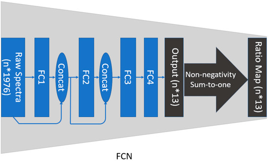
Figure 2.
The Raman spectrum decomposition using fully connected network (FCN). The Raman spectrum library was composed of 13 components with 1976 bands each.
2.4. Implementation
2.4.1. Loss Function
To optimally quantify the differences between predicted and ground truth ratios of components during training, an effective loss function , which facilitates model convergence combining the advantages of both and losses together, was used in this study [21,22].
and are the matrices of predictions and ground truth data, respectively; and are the number of rows and columns of each matrix.
Binary Cross Entropy loss was chosen to measure classification performance of DeepRaman.
2.4.2. Training
The FCN model was implemented in the Pytorch framework, and the weights of the encoder were randomly initiated by default [23]. The training process stopped until the losses had no longer decreased any further for over 500 epochs. For fair comparison, DeepRaman was also implemented in Pytorch and trained and validated on the same datasets as the FCN.
2.4.3. Evaluation Metrics
A mean absolute error (MAE), which measures the magnitude of differences between predicted and ground truth ratios, was used in this study. The overall accuracy (OA) was used to assess the performance of component identification [15].
Since DeepRaman is a classification model and is only specialized in component identification, we did not compare the ratio quantification as described in the study introducing this method [15], because once the components become wrongly identified by DeepRaman, the quantification by an NN-EN on these components is meaningless. Therefore, we separately compared the performance of component identification with DeepRaman and contrasted the component quantification performance with an NN-EN by assigning the ground truth number of components and corresponding spectra.
3. Results and Discussion
3.1. The Optimized Models of FCN and DeepRaman
The model was trained on simulated mixtures of Raman spectra with varying number of components, from 1 to 13, and with randomly assigned ratios from 0 to 1 to each component. The optimized FCN achieved of 0.000267 and 0.000262 on training and validation data, respectively (Figure 3, Table 1). The custom, optimized DeepRaman model trained on the same datasets showed BCE losses of 0.0598 and 0.0482 on training and validation data, respectively.
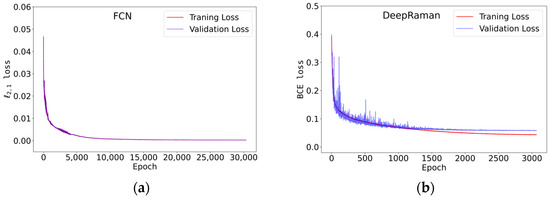
Figure 3.
The learning history of both FCN and DeepRaman. Blue and red solid lines indicate the changes in validation and training losses, in FCN (a) and BCE loss in DeepRaman (b), respectively, over the learning process.

Table 1.
The losses of FCN and DeepRaman on training and validation datasets.
3.2. Comparisons between FCN and NN-EN in Component Quantification
The mixed spectra were accurately decomposed into ratios of corresponding components with average MAEs ranging from 0.0 to 0.000733 (Table 2). Examples of these ground truth (GT) and predicted ratios of components from mixtures across different multi-component mixtures are shown in Figure 4. A slight error increase was observed with an increasing complexity of the input spectra. Peak errors of the FCN’s predictions were found in mixtures with five-component combinations. However, the MAE began to decrease as the complexity of mixtures increased further, due to the smaller component ratios (Table 2). For NN-EN [14], the MAE of estimated ratios increased consistently with the number of components in a mixture. The FCN had more precise predictions than the NN-EN in mixtures at all levels of complexity except for single-component mixtures. The average MAE of ratios estimated by the NN-EN was over one order of magnitude higher than that of the FCN. The best performance of the NN-EN was on the prediction of single-component mixtures, and it was on-par with the FCN.

Table 2.
Comparison of the performance of the fully connected network (FCN) and the non-negative elastic net (NN-EN) by the magnitude of mean absolute error (MAE) in quantifying the component ratio across various mixture complexities.
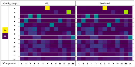
Figure 4.
Predicted component ratios of the synthetic spectra. The amplitudes of the ratios quantify the contributions of components to the input spectrum. Num_comp is the number of components used to generate the spectra of synthetic mixtures; Component No. indicates the i-th component inside the Raman spectrum library.
It is worth noting that the FCN was able to estimate the ratios of components in mixtures generated from different numbers of components based on their spectra without preprocessing steps. In contrast, smoothing and baseline removal were needed for the NN-EN to estimate component ratios. Additionally, the NN-EN required the exact number and the corresponding spectra of these components to conduct component ratios’ estimation, limiting its potential in real-world applications. On the contrary, once the FCN has been trained on a library, it could predict the ratios of components from any mixture composed of any random number of components from the library. The most valuable aspect was the high precision of the FCN in components’ ratio prediction compared to the NN-EN.
3.3. Comparisons between FCN and DeepRaman on Component Identification
DeepRaman is a dedicated component identification model and was tested to identify components of different categories in mixtures. However, it did not perform as well on our customized data as reported in the original paper. We further fine-tuned DeepRaman on the same dataset (including training and validation sets) used for the development of the FCN model.
Besides the precise estimation of ratios of different components of a mixture, the identities of components were determined based on the predicted non-zero ratios (Figure 4). Moreover, it is important to set a detective ratio threshold (DRT). First, the signal of a component can be easily deteriorated by other coexisting components with larger ratios inside a mixture. Second, smaller values are more prone to models’ prediction errors, resulting in wrong component identifications. Both classification, like DeepRaman, and regression, like FCN, models can potentially take advantage of setting optimal DRTs.
To achieve the best component identification performance of both FCN and DeepRaman, we tested 11 DRTs ranging from 0 to 1% with an increase of 0.1%. DeepRaman achieved its best performance with an OA of 83.1% at the DRT was 0.4% (Table 3). Similarly, the FCN benefited from setting the DRT with an average OA increasing from 95.5% to the best OA of 99.7 at DRTs of 0.7%,0.8% or 1% (Table 4). Moreover, the average OAs of the FCN in components’ identification were within a relatively small range of 1.6% difference after setting DRTs above 0. At the same time, the lowest average OA of the FCN in component identification was 98.1%, which is 16% higher than the optimal identification performance of DeepRaman after setting a DRT.

Table 3.
Overall accuracy (OA) of the DeepRaman model under 11 different detectable ratio thresholds (DRTs).

Table 4.
Overall accuracy (OA) of the FCN model under 11 different detectable ratio thresholds (DRTs).
Setting the DRT helped remove the components that were hard to be identified by DeepRaman increasing the average OA from 77.8% to 79.9%, as the DRT increased from 0 to 0.1%. However, the average OA started decreasing after reaching the peak performance at 83.8%. The main reason could be that DeepRaman was still excellent in component identification, and components with ratios higher than 0.4% could not be neglected. When the complexity level of the input mixture increased, more components were classified with ratios below a DRT (Figure 5). The deterioration of DeepRaman’s accuracy occurred mainly in more complex mixtures, as shown in Table 3. On the contrary, the increase in accuracy was noticed mainly for mixtures with less components, as setting the DRT helped remove noisy predictions.
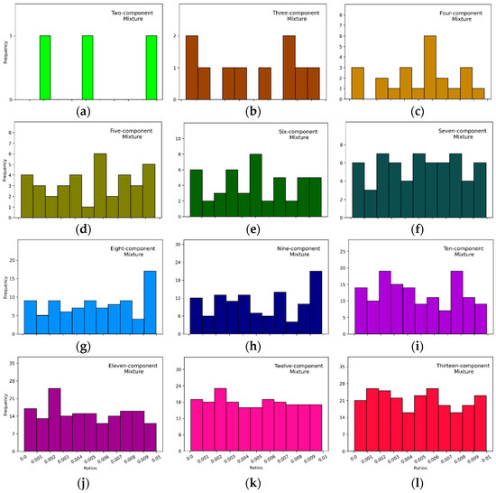
Figure 5.
Frequencies of component ratios below the maximum DRT, 1%, in 3600 Raman mixtures in testing data. (a–l) represent different numbers of components from 2 to 13 in the mixture.
Compared to the FCN, DeepRaman suffered severely when the number of components inside a mixture increased. The OA of component identification decreased from 100% for single-component mixtures to 80.3% for mixtures of 13 different components with a DRT set at 0.4%. Although there were minor fluctuations in the OA as the input mixture complexity increased, they were negligible compared to the significant changes observed in DeepRaman. This highlights the robustness of the FCN to varying complexity levels of the input mixtures.
Unlike methods to compare the similarity between a composite spectrum and spectra of all potential components, the component identification by the FCN in our study fully relied on the estimated component ratios and is illustrated in two examples: single-component (Figure 6) and thirteen-component decomposition (Figure 7). Due to the high quantification performance of the FCN, components identification was also highly accurate, especially when an appropriate DRT was set. Both the FCN and DeepRaman required an optimal DRT for the best performance (Table 1 and Table 2); however, the FCN was more robust to the DRT change and had much better performance under different DRT settings compared to DeepRaman.
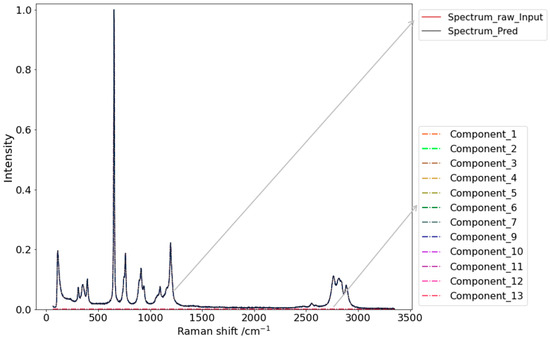
Figure 6.
Example of the decomposition of a single-component (Component_8) input spectrum. Spectrum_raw_Input represents the input unprocessed spectrum; Spectrum_Pred is the spectrum generated based on the predicted ratios and corresponding spectrum of the library. Conpunent_1 to Component_13 represent the thirteen components of the Raman spectrum library.
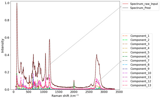
Figure 7.
Example of the identification of a thirteen-component input spectrum with DRT of 0.7%. Spectrum_raw_Input represents the input unprocessed spectrum; Spectrum_Pred is the spectrum generated based on the predicted ratios and corresponding spectra of the library. Conpunent_1 to Component_13 represent the thirteen components of the Raman spectrum library.
The proposed modeling approach combats both quantification and identification based on raw spectra simultaneously, which is advantageous compared to the previous studies, which focused only on either preprocessing [18], component identification [7,14,15,24] or decomposition [10]. The single-step approach also makes further deployment easier as it does not rely on other analytical, (e.g., NN-EN) or different preprocessing methods (noise and baseline removal). In addition, the speed of the FCN is close to real time, as it only takes 140 ms to process 300 samples, which further supports its potential in real-world applications.
The model itself is not generalizable due to the limited size of the library used in this study. However, the effectiveness of the method used in this study has been well-validated through detailed comparisons with DeepRaman and the NN-EN. To find a generalized model that fits all different types of data is literally inconceivable in practice. It is encouraged to apply the method proposed in this study on real-world applications and fine tune it to reach its potential.
4. Conclusions
We proposed an effective FCN to decompose multi-component raw Raman spectra comprising random number of components from a fixed library. The developed model quantified the content of different components more precisely compared to the well-established NN-EN method, with no preprocessing needed. The component identification performance of FCN was also more accurate and showed much less degradation of performance with increasing mixture complexity, when compared to the recently published DeepRaman. Our model overcame the classical multistep Raman spectrum decomposition and managed both component identification and quantification from an unprocessed Raman spectrum in a single run. The effectiveness of our modeling approach has been tested in a simulation study using simple chemical compounds, and future studies will verify its practical applicability for mixtures of chemically more complex samples.
Author Contributions
J.Z.: conceptualization, software, formal analysis, writing—original draft, review and editing; K.K.: conceptualization, writing−review and editing. All authors have read and agreed to the published version of the manuscript.
Funding
This research was supported by internal funds of NIBIO and the Norwegian Research Council’s base funding [Contract No. 342631/L10].
Data Availability Statement
The code is available at: https://github.com/ZJiangsan/RamanSpectrumDecompositionFromRaw (accessed on 1 August 2024).
Conflicts of Interest
The authors declare no conflicts of interest.
References
- Lawson, L.S.; Rodriguez, J.D. Raman Barcode for Counterfeit Drug Product Detection. Anal. Chem. 2016, 88, 4706–4713. [Google Scholar] [CrossRef] [PubMed]
- Galeev, R.R.; Semanov, D.A.; Galeeva, E.V.; Falaleeva, T.S.; Aryslanov, I.R.; Saveliev, A.A.; Davletshin, R.R. Peak Window Correlation Method for Drug Screening Using Raman Spectroscopy. J. Pharm. Biomed. Anal. 2019, 163, 9–16. [Google Scholar] [CrossRef] [PubMed]
- Wang, Y.; Fan, X.; Tian, S.; Zhang, H.; Sun, J.; Lu, H.; Zhang, Z. EasyCID: Make Component Identification Easy in Raman Spectroscopy. Chemom. Intell. Lab. Syst. 2022, 231, 104657. [Google Scholar] [CrossRef]
- Grotch, S.L. Matching of Mass Spectra when Peak Height is Encoded to One Bit. Anal. Chem. 1970, 42, 1214–1222. [Google Scholar] [CrossRef]
- Li, B.; Schmidt, M.N.; Alstrøm, T.S. Raman Spectrum Matching with Contrastive Representation Learning. Analyst 2022, 147, 2238–2246. [Google Scholar] [CrossRef]
- Samuel, A.Z.; Mukojima, R.; Horii, S.; Ando, M.; Egashira, S.; Nakashima, T.; Iwatsuki, M.; Takeyama, H. On Selecting a Suitable Spectral Matching Method for Automated Analytical Applications of Raman Spectroscopy. ACS Omega 2021, 6, 2060–2065. [Google Scholar] [CrossRef]
- Chen, T.; Baek, S.-J. Library-Based Raman Spectral Identification Using Multi-Input Hybrid ResNet. ACS Omega 2023, 8, 37482–37489. [Google Scholar] [CrossRef]
- Sin, S.Y.; Widjaja, E.; Yu, L.E.; Garland, M. Application of FT-Raman and FTIR Measurements Using a Novel Spectral Reconstruction Algorithm. J. Raman Spectrosc. 2003, 34, 795–805. [Google Scholar] [CrossRef]
- Zhang, Z.-M.; Chen, X.-Q.; Lu, H.-M.; Liang, Y.-Z.; Fan, W.; Xu, D.; Zhou, J.; Ye, F.; Yang, Z.-Y. Mixture Analysis Using Reverse Searching and Non-Negative Least Squares. Chemom. Intell. Lab. Syst. 2014, 137, 10–20. [Google Scholar] [CrossRef]
- Zeng, H.; Hou, M.; Ni, Y.; Fang, Z.; Fan, X.; Lu, H.; Zhang, Z. Mixture Analysis Using Non-negative Elastic Net for Raman Spectroscopy. J. Chemom. 2020, 34, e3293. [Google Scholar] [CrossRef]
- Bratchenko, L.A.; Bratchenko, I.A.; Khristoforova, Y.A.; Artemyev, D.N.; Konovalova, D.Y.; Lebedev, P.A.; Zakharov, V.P. Raman Spectroscopy of Human Skin for Kidney Failure Detection. J. Biophotonics 2021, 14, e202000360. [Google Scholar] [CrossRef] [PubMed]
- Tahir, M.A.; Dina, N.E.; Cheng, H.; Valev, V.K.; Zhang, L. Surface-Enhanced Raman Spectroscopy for Bioanalysis and Diagnosis. Nanoscale 2021, 13, 11593–11634. [Google Scholar] [CrossRef] [PubMed]
- Nava, V.; Frezzotti, M.L.; Leoni, B. Raman Spectroscopy for the Analysis of Microplastics in Aquatic Systems. Appl. Spectrosc. 2021, 75, 1341–1357. [Google Scholar] [CrossRef]
- Fan, X.; Ming, W.; Zeng, H.; Zhang, Z.; Lu, H. Deep Learning-Based Component Identification for the Raman Spectra of Mixtures. Analyst 2019, 144, 1789–1798. [Google Scholar] [CrossRef]
- Fan, X.; Wang, Y.; Yu, C.; Lv, Y.; Zhang, H.; Yang, Q.; Wen, M.; Lu, H.; Zhang, Z. A Universal and Accurate Method for Easily Identifying Components in Raman Spectroscopy Based on Deep Learning. Anal. Chem. 2023, 95, 4863–4870. [Google Scholar] [CrossRef]
- Luo, R.; Popp, J.; Bocklitz, T. Deep Learning for Raman Spectroscopy: A Review. Analytica 2022, 3, 287–301. [Google Scholar] [CrossRef]
- Pan, L.; Pipitsunthonsan, P.; Zhang, P.; Daengngam, C.; Booranawong, A.; Chongcheawchamnan, M. Noise Reduction Technique for Raman Spectrum Using Deep Learning Network. In Proceedings of the 2020 13th International Symposium on Computational Intelligence and Design (ISCID), Hangzhou, China, 12–13 December 2020; IEEE: Piscataway, NJ, USA, 2020; pp. 159–163. [Google Scholar]
- Chen, T.; Son, Y.; Park, A.; Baek, S.-J. Baseline Correction Using a Deep-Learning Model Combining ResNet and UNet. Analyst 2022, 147, 4285–4292. [Google Scholar] [CrossRef]
- Gebrekidan, M.T.; Knipfer, C.; Braeuer, A.S. Refinement of Spectra Using a Deep Neural Network: Fully Automated Removal of Noise and Background. J. Raman Spectrosc. 2021, 52, 723–736. [Google Scholar] [CrossRef]
- Vaswani, A.; Shazeer, N.; Parmar, N.; Uszkoreit, J.; Jones, L.; Gomez, A.N.; Kaiser, Ł.; Polosukhin, I. Attention Is All You Need. Adv. Neural Inf. Process Syst. 2017, 30. [Google Scholar]
- Zhao, J.; Qu, Y.; Ninomiya, S.; Guo, W. Endmember-Assisted Camera Response Function Learning, Toward Improving Hyperspectral Image Super-Resolution Performance. IEEE Trans. Geosci. Remote Sens. 2022, 60, 1–14. [Google Scholar] [CrossRef]
- Qu, Y.; Qi, H.; Kwan, C.; Yokoya, N.; Chanussot, J. Unsupervised and Unregistered Hyperspectral Image Super-Resolution with Mutual Dirichlet-Net. IEEE Trans. Geosci. Remote Sens. 2021, 60, 1–18. [Google Scholar] [CrossRef]
- Paszke, A.; Gross, S.; Massa, F.; Lerer, A.; Bradbury, J.; Chanan, G.; Killeen, T.; Lin, Z.; Gimelshein, N.; Antiga, L. Pytorch: An Imperative Style, High-Performance Deep Learning Library. Adv. Neural Inf. Process. Syst. 2019, 32. [Google Scholar]
- Liu, J.; Osadchy, M.; Ashton, L.; Foster, M.; Solomon, C.J.; Gibson, S.J. Deep Convolutional Neural Networks for Raman Spectrum Recognition: A Unified Solution. Analyst 2017, 142, 4067–4074. [Google Scholar] [CrossRef] [PubMed]
Disclaimer/Publisher’s Note: The statements, opinions and data contained in all publications are solely those of the individual author(s) and contributor(s) and not of MDPI and/or the editor(s). MDPI and/or the editor(s) disclaim responsibility for any injury to people or property resulting from any ideas, methods, instructions or products referred to in the content. |
© 2024 by the authors. Licensee MDPI, Basel, Switzerland. This article is an open access article distributed under the terms and conditions of the Creative Commons Attribution (CC BY) license (https://creativecommons.org/licenses/by/4.0/).