Abstract
To establish a high-precision prediction model for the material removal rate (MRR) of TC4 titanium alloy material in vertical vibratory finishing equipment, an orthogonal experiment was conducted using TC4 titanium alloy plate as the experimental specimen. We performed variance analysis of the impact of vibration frequency, the phase difference, the mass of upper eccentric block, and the mass of lower eccentric block on the MRR. We then drew the main effect diagram and analyzed the influence of various process parameters on the MRR. Mathematical regression and a neural network were used to construct predictive models for the MRR with respect to process parameters, and a genetic algorithm (GA) was coupled to optimize the neural network to improve the predictive performance of the model. By calculating the R2, validating the set sample prediction error, and averaging the absolute percentage error (MAPE) of each model, it was found that the neural network model had better prediction performance than the mathematical regression model, with an accuracy of 82.2%. After coupling with the GA, the prediction accuracy reached 95.5%. The research results indicated that, compared with mathematical regression and the original neural networks, the neural network coupled with the GA had better predictive performance, providing an effective method for predicting the MRR in vertical vibratory finishing.
1. Introduction
TC4 titanium alloy is characterized by its light weight, outstanding corrosion resistance, and high strength. Owing to these remarkable properties, it finds extensive applications in numerous components of aero-engines. Common TC4 titanium alloy finishing technology includes vibratory finishing, abrasive flow finishing, and shot peening [1]. As a typical finishing process, vibratory finishing stands out for its robust adaptability and remarkable processing efficacy. It can achieve burr removal, surface polishing, and surface strengthening, and has been widely used in the finishing process of various aero-engine components [2,3,4]. As the material removal rate (MRR) is an important index reflecting the efficiency of finishing, it is a key factor in selecting process parameters [5]. Therefore, taking the MRR as the research object, we analyzed the method of constructing the relationship model between the process parameters and the machining effect.
The process parameters that affect the MRR include the equipment, specimen, and granular media. In terms of the specimen parameter, Li [6] carried out finishing on aluminum alloy specimens with different initial milling surfaces, and found that the initial surface roughness had an impact on the processing parameters and machining results. In terms of the granular media parameter, Wang [7] explored the physical properties of different materials of granular media. It was discovered that granular media of different materials exhibited distinct disparities in their impacts on the surface roughness and surface element processing. Specifically, the specimens processed with white ceramic granular media had the highest brightness. Hao [8] conducted a study on the impact of the elasticity coefficient, density, and rolling friction coefficient of the granular media on the average contact force. The findings revealed that the average contact force increased as the density and the resilience coefficient increased, while it decreased with the growth of the rolling friction coefficient. In terms of the granular media parameter, Maciel [9] delved into the impact of the container’s amplitude and frequency on the movement of the granular media during vibration machining. The research revealed that the velocity of the granular media was closely correlated with the container’s movement. Among the above parameters, equipment parameters are the most fundamental influencing factors, so many researchers have focused on the study of equipment parameters to analyze their impact on the processing effect.
Due to the complex dynamic behavior of the granular media in the processing process, there is a nonlinear mapping relationship between the equipment parameters and the MRR. The selection of equipment parameters is mainly determined by experience, and the MRR is difficult to predict, which restricts the high-end application of the vibratory finishing [5]. Consequently, researchers have explored the correlation between the parameters of vibratory finishing equipment and the machining effect from diverse perspectives. In terms of theoretical research, Zhang [10], through the dynamic analysis of the physical model built by the vertical vibratory finishing equipment, discovered that when the phase angle of the eccentric block was 67°, the motion velocity of the granular medium reached the maximum and moved in a stable manner. This condition was deemed suitable for the processing of workpieces. Tian [11] obtained the optimal fixed position and direction of the workpiece through theoretical analysis, and conducted experimental verification to obtain the optimal surface roughness of 0.52 μm. In terms of experimental research, numerous scholars have altered the fixed position of the workpiece, as well as the parameters of the granular media and equipment. Through these adjustments, they have delved into how equipment parameters impact the movement of the granular media and the forces involved. Subsequently, they have investigated the influence of the MRR, ultimately determining the appropriate equipment parameters [12,13,14,15]. In terms of simulation research, Hashemnia [16] employed the discrete element software EDEM to conduct simulations and experiments on the velocity of the granular medium and the overall flow velocity in vibratory finishing. The final discrepancies between the simulation results and the experimental data for these two aspects were 19% and 30% respectively. Maciel [9] studied the effect of the container on the velocity of the granular medium in the vibratory finishing through discrete element simulation, providing guidance for exploring the influence of process parameters on MRR. At present, most of the research methods on the relationship between the MRR and equipment parameters are qualitative research. After obtaining the MRR trend, along with equipment parameters, the appropriate parameter range is determined. However, the mapping relationship between the two cannot be accurately established, and it cannot be used for the numerical prediction of the MRR.
To precisely establish the mapping relationship, a number of scholars have resorted to mathematical regression methods to construct the prediction model for the MRR. Tang [17] built a regression model for the MRR, and the model R2 reached 0.937, which had an excellent degree of fit. Naeim [18] used multiple regression to construct the MRR prediction model. Subsequently, the process parameters were analyzed based on this model, and the optimal combination of process parameters was determined. In addition, neural networks with self-learning and adaptive ability are also widely used to establish various mapping relationships. Many scholars have introduced the neural network into different processing methods to predict the processing effect, and the prediction accuracy has reached more than 90% [19,20,21,22,23]. Both Kanovic [24] and Harlal [25] compared the neural network with the traditional regression model and found that the prediction accuracy of the neural network was higher. Nevertheless, the traditional neural network model exhibits several drawbacks during the training process. For instance, its prediction performance is unstable, the model convergence is poor, and it is highly prone to overfitting. Given these issues, optimizing the calculation method of the traditional neural network becomes essential. As an intelligent optimization algorithm, the genetic algorithm (GA) can be used to optimize all kinds of parameters. By using the GA to optimize the weight and bias of neural network, many scholars have improved the prediction accuracy of the model [26,27,28]. Currently, this kind of method lacks practical application experience in the prediction of the MRR of vertical vibratory finishing, so the research is still in the exploration stage.
The purpose of this paper was to build a model for predicting the removal rate of TC4 material by vertical vibratory finishing equipment parameters. On the basis of an orthogonal experiment, the influence of the vibration frequency, phase difference of the eccentric block, mass of upper eccentric block, and mass of lower eccentric block on the MRR were analyzed by variance. A prediction model was constructed according to mathematical regression and the neural network, and the GA were coupled to optimize the neural network, so as to improve the prediction accuracy of the neural network. By introducing the validation samples and computing the prediction error under each model, the accuracy of the models was verified, and their prediction performances were compared and analyzed. The method presented in this paper provides the basis for constructing the prediction model of the vertical vibratory finishing process parameters.
2. Principle of Vertical Vibratory Finishing
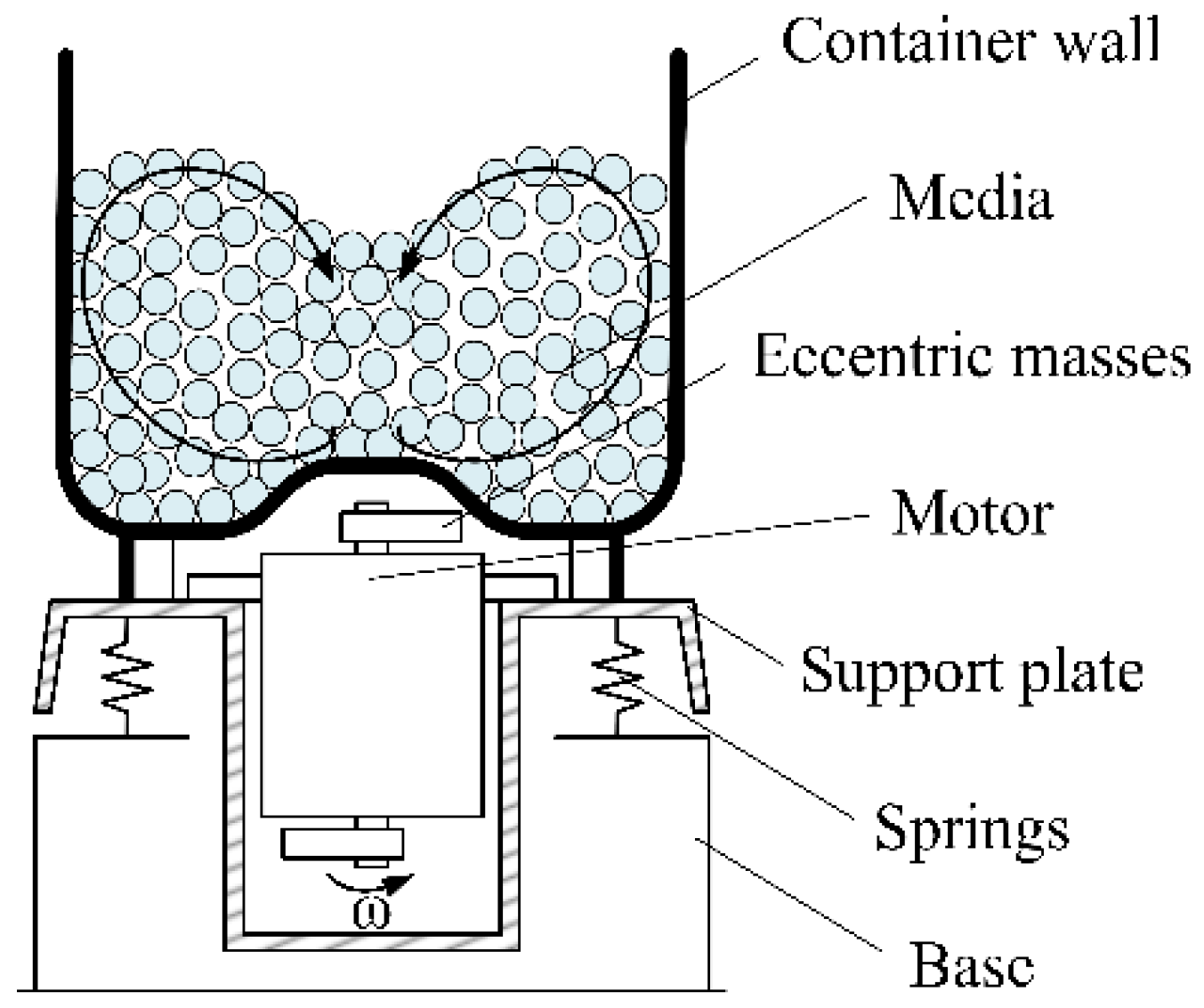
Figure 1 is a schematic diagram of the vertical vibratory finishing processing equipment. It is driven by a vertically mounted vibration motor, which is equipped with eccentric blocks with a certain angle in the horizontal plane at both ends of the shaft. During the processing stage, the exciting motor rotates at high speed, causing the container to generate complex periodic vibrations. These vibrations drive the granular medium, the workpiece, and the liquid medium within the container to move along a circular spiral track. The granular medium produces rolling, micro-grinding, and collision with the workpiece to realize the surface finishing of the workpiece [5].

Figure 1.
Vertical vibratory finishing equipment diagram.
The reason for the complex vibration of the container is that during the operation of the equipment, the exciting motor produces centrifugal exciting force and torque in the horizontal and vertical planes. The exciting force induces the granular medium and the workpiece within the container to generate a rotational motion around the central axis. Simultaneously, the torque causes the granular medium and the workpiece in the container to exhibit a rolling motion. The calculation formula of exciting force and exciting moment is shown in Equations (1) and (2) [5]:
where ω is the motor speed, r is the distance from the center of mass to the axis of the eccentric block, α is the angle between the eccentric block and the horizontal plane, m0 is the mass of eccentric block, l0 is the vertical distance between eccentric blocks, and l is the distance between the upper eccentric block and the center of mass.
3. Experiment
3.1. Experimental Specimen and Processing Environment
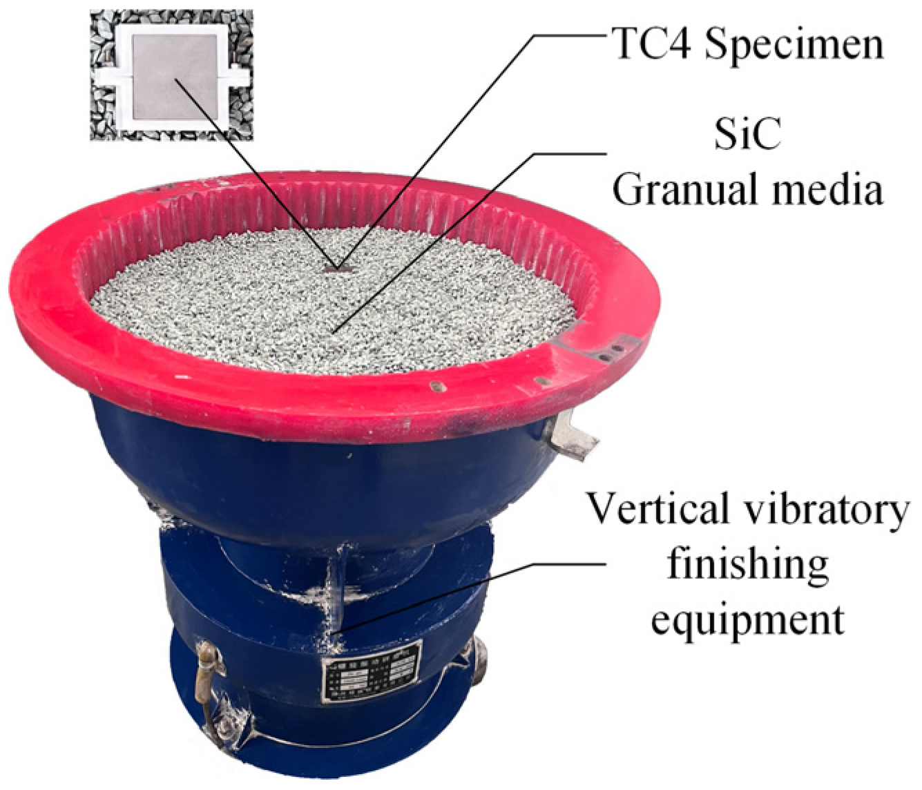
TC4 titanium alloy was used as the test specimens, with a size of 40 mm × 40 mm × 5 mm. Prior to vibratory finishing, the test specimens were machined using identical milling parameters. This ensured that the initial surface quality of all specimens was consistent. ZK-60 vertical vibratory finishing equipment was used for processing. In order to control the residual elements on the surface of the machined parts, granular medium of the silicon carbide (SiC) type is used. Wang [29] found that granular media in the shape of oblique triangles had excellent processing efficiency. Moreover, the research shows that the contact force on the workpiece increases as the size of the granular medium increases, and the processing efficiency is faster, but the surface roughness of the machined parts will continue to increase [30]. Therefore, silicon carbide oblique triangular granular medium (4 mm × 4 mm) was used for processing. The experimental processing conditions are shown in Table 1, and the experimental processing environment is shown in Figure 2. In the experiment, only one side of the specimen was machined, and the other side was protected by the fixture. When machining, we placed the workpiece along the edge and poured on the appropriate amount of HYF grinding liquid and water.

Table 1.
Experimental conditions for vertical vibration finishing.

Figure 2.
Experimental processing environment.
3.2. Process Parameters and Experimental Design
According to Equations (1) and (2), factors that affect the exciting force and torque include the motor speed (ω), the angle between the two eccentric blocks (α), the mass of the upper eccentric block (ma), and the mass of the lower eccentric block (mb). These parameters affect the vector sum of the exciting force and torque, and the motion law of the container. Therefore, the above parameters were used as the process parameter variables. To study these four factors, five levels of orthogonal experiments were designed with the appropriate variable level range. Based on experimental inquiry, if the vibration frequency is excessively high, the motor will be overloaded. Conversely, if the vibration frequency is too low, the granular medium within the container will have difficulty in moving. Therefore, the vibration frequency range was determined from 15 Hz to 25 Hz. To guarantee the stable operation of the container after increasing the eccentric mass, the mass range of the eccentric mass was determined from 0.9 kg to 1.9 kg. Previous research has indicated that the speed of the granular medium in the container was fastest when the phase difference of the eccentric block was 67° [6]. Therefore, with the eccentric block phase difference of 60° as the center, the range was determined from 0° to 120°. Experimental variables and ranges are shown in Table 2.
Table 2.
Experimental variables.
The mass of the TC4 titanium alloy specimen before and after processing was measured by high-precision electronic balance. Subsequently, the MRR of the specimen under each process parameter was recorded and calculated. Ultrasonic cleaning and drying were carried out before each measurement to reduce the influence of surface residues on the surface quality of test specimens. According to the measured result, the MRR was converted into the material removal depth per unit time and area, and the calculation formula is shown in Equation (3).
where m0 is the mass before processing, m1 is the quality after processing, t is processing time, ρ is the density of the specimen, and S is the specimen processing area.
4. The Prediction Model of MRR
4.1. Experimental Results and Analysis
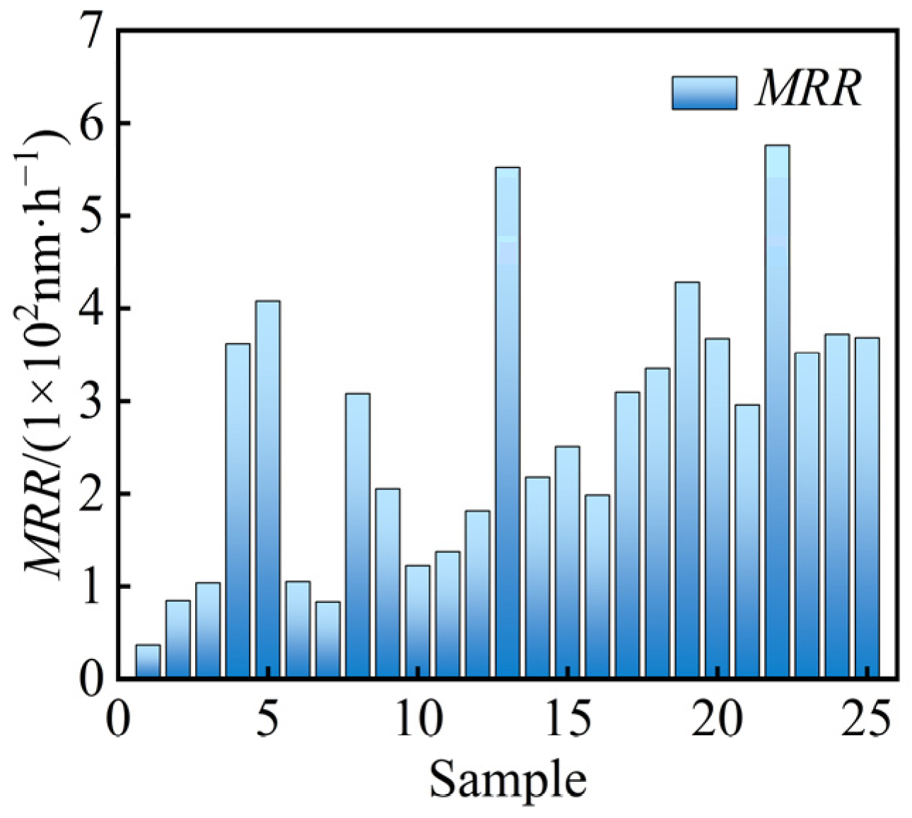
After finishing, the surface quality of the specimens was improved to varying degrees. The processing effects of different parameters were compared and analyzed according to the corresponding MRR of the specimens processed under different parameters. The results are shown in Table 3. In order to facilitate the analysis of the distribution of the MRR under different process parameters, the distribution diagram shown in Figure 3 was drawn.
Table 3.
Orthogonal experimental results.

Figure 3.
Distribution of MRR.
By analyzing the experimental data in tandem with the MRR distribution diagram, it becomes evident that the MRR experienced a marked increase when both the mass of the eccentric block and its vibration frequency reached their peak values. The reason for this is that the exciting force increased monotonically with the mass of the eccentric block and increased quadratically with the vibration frequency. As the exciting force grew, the vibration of the granular medium within the container strengthened. This caused the granular medium to move more vigorously, thereby enhancing the processing efficiency. However, due to the mismatch between the eccentric block quality and the phase difference under some parameters, the exciting force was weakened when the rotational speed was very high or the eccentric block mass was very large, the vibration intensity of the granular media was reduced, and the MRR was reduced, resulting in energy waste.
The influence of different process parameters on the MRR was analyzed by variance, and the most influential process parameters were determined. According to the analysis, the F value of different parameters affecting the MRR were as follows: vibration frequency (3.372), eccentric block phase difference (2.033), mass of lower eccentric block (1.416), and mass of upper eccentric block (1.112). All four process parameters exerted distinct influences on the MRR. Notably, the MRR exhibited a higher degree of sensitivity to the vibration frequency.
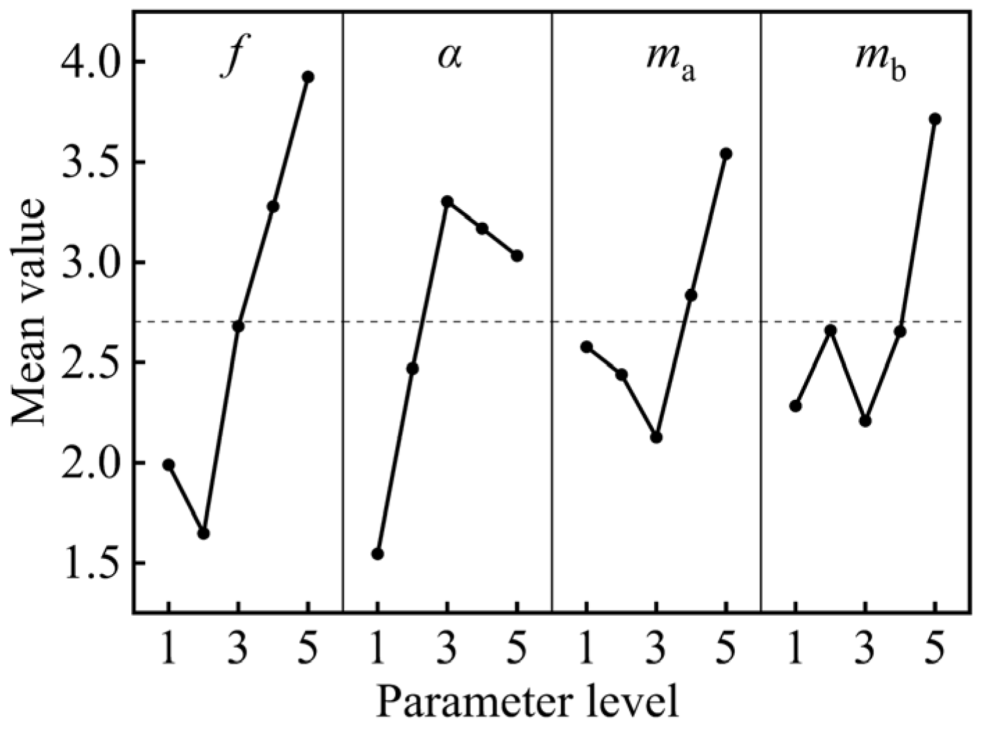
The main effect diagram of the MRR is shown in Figure 4. It can be seen from the figure that the MRR decreased first and then increased with vibration frequency. The underlying cause was that when the vibration frequency was low, the amplitude of the container was relatively large. However, as the vibration frequency increased, the amplitude of the container reduced, consequently resulting in a decline in the MRR. As the vibration frequency rose, the MRR experienced a remarkable increase. With the growth of the eccentric block phase difference, the MRR first increased and then decreased, hitting its peak when the eccentric block phase difference α = 60°. This is because when the eccentric block phase difference was around 60°, the granular medium has the highest flow rate, and the workpiece was under stress, which jointly contributed to this change in the MRR. In addition, with the growth of the mass of the upper eccentric block, the MRR first increased and then decreased, hitting its peak when the mass of the upper eccentric block ma = 1.4 kg. The reason for this was that when the mass of the upper eccentric block was less than 1.4 kg, the comprehensive influence of other parameters was more significant. However, once it exceeded 1.4 kg, the mass of the upper eccentric block became the primary source of the excitation force. This led to the intensification of container vibration and an increase in the MRR. Following this, when the mass of the lower eccentric block was small, the excitation force acting on the container was weak. In this case, the MRR was influenced by all process parameters, yet no obvious change could be observed. Once the mass of the lower eccentric block surpassed 1.4 kg, the excitation force produced by the lower eccentric block escalated and became the dominant force. As a result, the vibration intensity of the container increased, and the MRR increased monotonically in tandem.

Figure 4.
Main effect of MRR.
Through comprehensive analysis, it can be concluded that the vibration frequency, the phase difference of the eccentric block, the mass of the upper eccentric block, and the mass of the lower eccentric block all exerted distinct influences on the MRR. Therefore, they could be fed into the neural network as the primary regulatory parameters.
4.2. MMR Prediction Model Based on Mathematical Regression
A regression model is a statistical data analysis method, which can greatly improve the efficiency of process research [18]. In this paper, three types of models were utilized for analysis: the pure quadratic model, the cross model, and the complete quadratic model. Subsequently, a comparison was made of the prediction accuracies of these models, with the objective of improving the applicability of the mathematical models within this specific context. According to the 25 groups of results of orthogonal experiments in Table 3, a mathematical regression model of the MRR was constructed. The equations are as follows:
A goodness-of-fit test was carried out on the three regression models, and the R2 values were 0.725, 0.737, and 0.769, respectively, all of which were between 0.7 and 0.8. The results indicated that the three regression models had similar fitting effects on the data. With the increasing number of fitting formula terms, R2 also increased gradually. The perfect quadratic model had the best fitting effect, and could be used to set the MRR prediction model.
4.3. MMR Prediction Model Based on GABP Neural Network
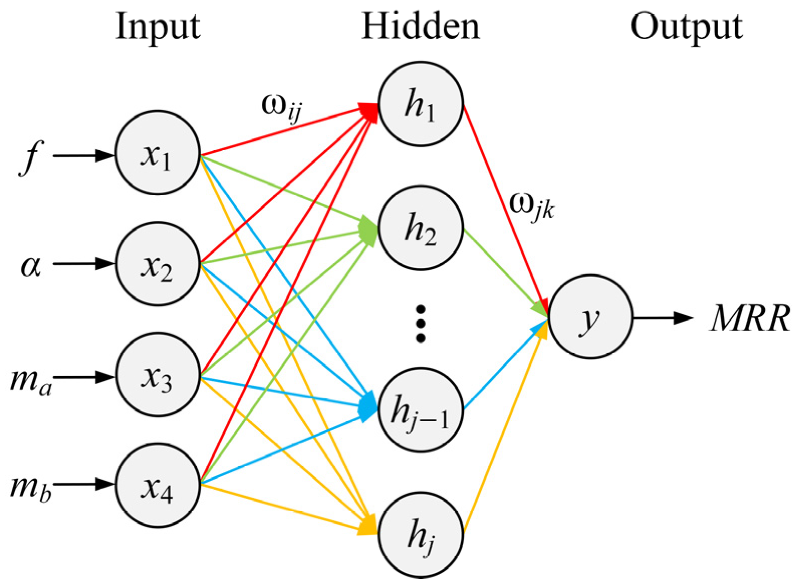
The neural network model consisted of an input layer, a hidden layer, and an output layer. The external data information entered the network through the input layer and was transmitted backward. After calculation and processing by the hidden layer, it was transmitted to the output layer, and the target data were outputted according to the transfer function of the output layer [31]. According to the biological evolution theory of “survival of the fittest”, a genetic algorithm calculates the fitness value by designing the fitness function, and selects the individual genes with the highest fitness by means of selection, crossover, and variation [32]. In this paper, a BP neural network was used to establish the prediction model. By combining the genetic algorithm (GA) with the neural network, the GABP neural network was established. This was able to improve the prediction performance of the original neural network.
The feedforwardnet function was utilized to construct the neural network. To optimize the mean square error (MSE) of the model and enhance the training efficiency, the trainlm function was adopted as the model training function. In order to ensure high prediction accuracy, the logsig function was used as the activation function of hidden layer neurons and the purelin function as the activation function of output layer neurons [33]. The maximum number of neural network training was set to 5000 times, and the rest conditions were default. The input layer of the network was configured with the following parameters: vibration frequency, phase difference, mass of the upper eccentric block, and mass of the lower eccentric block. The number of nodes in the input layer was set to four. Meanwhile, the output layer was defined as the MRR, and the number of nodes in the output layer was one. The neural network was established based on the orthogonal experiment, and its structure is shown in Figure 5. The different colored arrows in the Figure 5 indicate the weight coefficient of the neurons in the previous layer. Since an excessive number of nodes in the hidden layer can result in poor generalization ability of the network, while too few nodes will decrease the fitting capacity for complex functions, the range of the number of nodes in the hidden layer was determined according to Equation (7) [34]:
where α is the constant between 0 and 10, h is the number of hidden layer nodes, i is the number of nodes in the input layer, and k is the number of nodes in the output layer.
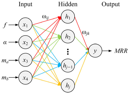
Figure 5.
Schematic of neural network structure.
We substituted the number of nodes in the input and output layers into the empirical formula to ascertain the range of the number of nodes in the hidden layer. The result determined a range of 3 to 13 layers. As shown in Figure 6, by training the neural network within the effective range, the mean square error (MSE) corresponding to the number of nodes in different hidden layers was summarized. The prediction error was compared comprehensively and the number of hidden layer nodes was ascertained to be 10. At this time, the network structure was 4-10-1 and the predicted MSE was 0.311.
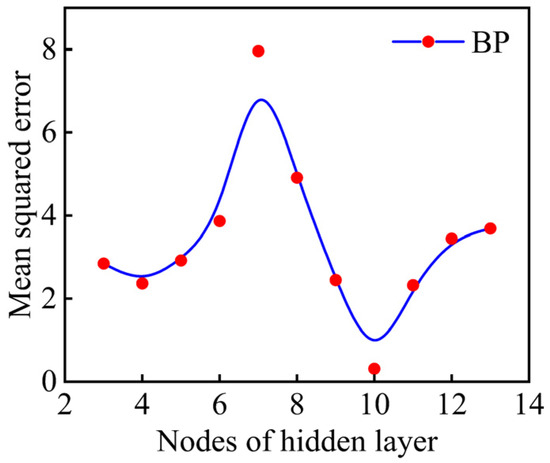
Figure 6.
Changes in mean square error.
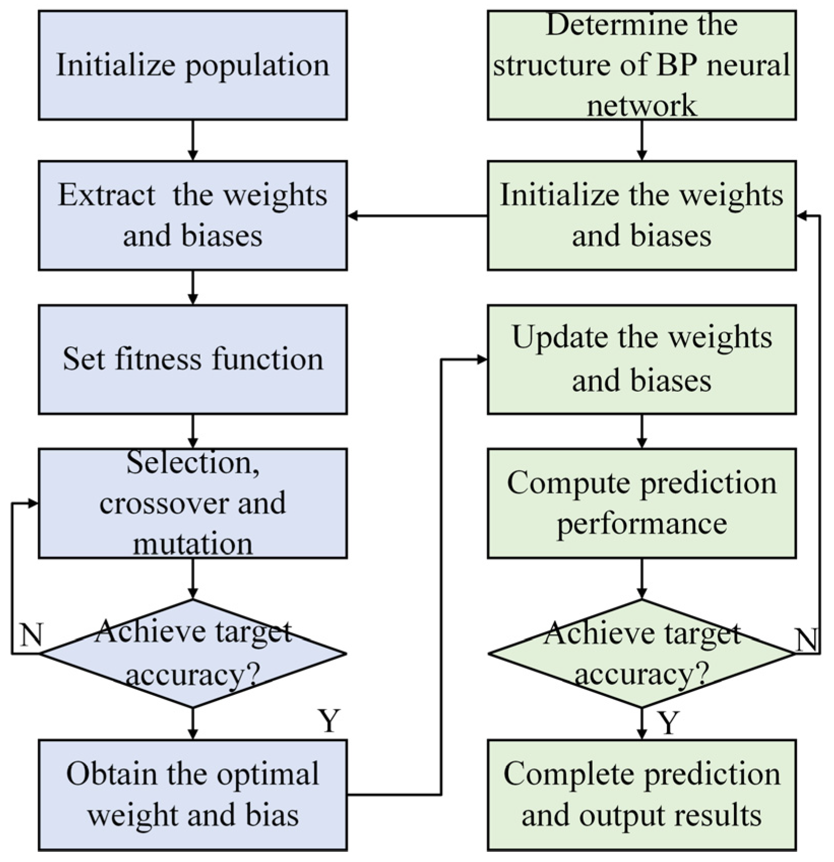
The coupling optimization process is shown in Figure 7. The weights and biases of each neuron in the neural network were extracted by functions such as net.iw, net.Iw, and net.b. These data were sorted into one-dimensional vectors in the GA. Since the analysis object was a small data sample, Set the initial population size to 50 and the maximum evolutionary algebra to 1000. For the GA, the default functions were used for selection, crossover, and variation. Specifically, the crossover probability was set to 0.1, and the mutation probability was set to 0.08. The MSE between the predicted values and the actual values of the neural network was defined as the fitness function to select the optimal genes.

Figure 7.
The flowchart of genetic algorithm coupled with optimization neural network.
The GA function was used to set the above parameters, and gene optimization was completed after selection, crossover, and mutation operations. The weight and bias matrix were replaced back into the original neural network for updating, retraining the model, and computing diverse prediction errors associated with it.
In MATLAB (R2021a), the weight and bias matrices of each neuron were extracted using the neural network toolbox. Subsequently, the abstract neural network model was converted into a mathematical calculation formula. The mathematical calculation formula is shown in Equations (8)–(10), and the weight and bias distribution are shown in Table 4. In Table 4, for the convenience of indicating heavy ownership, ω(2) is transposed and written as ω(2)T.
where X is the input parameter matrix, MRR is the predicted value of material removal rate, ω(i) is the weight of the neural network from layer i to layer i + 1, b(i) is the bias of the neural network from layers i to i + 1, and f(i)(x) is the activation function of the layer i to layer i + 1 neural network.
Table 4.
Distribution of weights and biases.
4.4. Comparative Analysis of Prediction Models
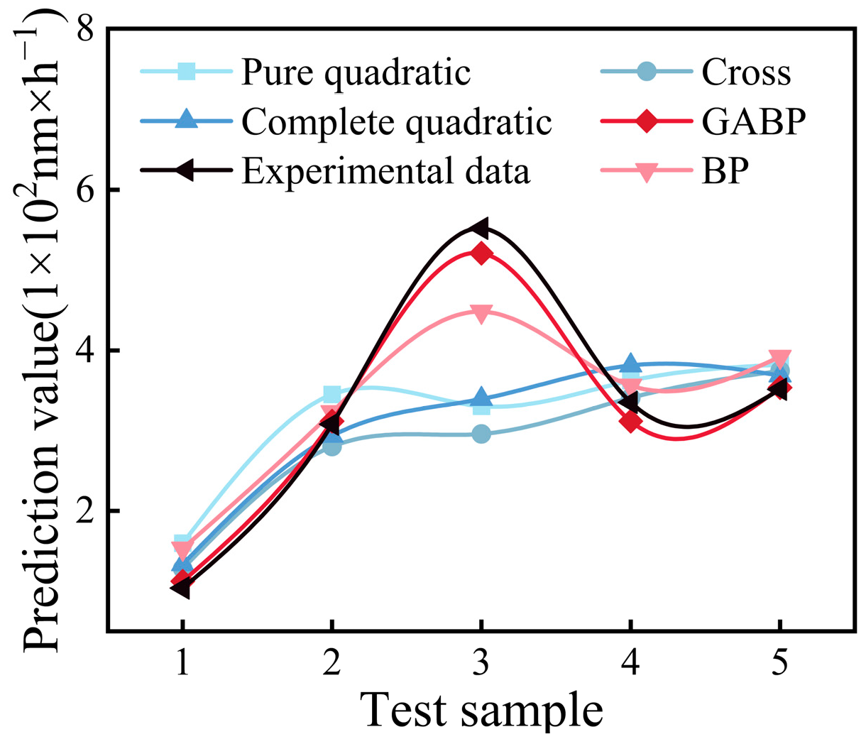
The 3rd, 8th, 13th, 18th, and 23rd data were selected as validation samples. These data subsets were then incorporated into various forecasting models for validation purposes. The prediction accuracy of the model was evaluated from two aspects: the prediction situation of the test samples and the whole average absolute percentage error (MAPE).
The MRR prediction model on the samples of the verification set is shown in Figure 8. The mathematical regression prediction model often showed poor accuracy when predicting the third sample in the validation set, with relative errors exceeding 35%. In contrast, the prediction model established by the neural network effectively enhanced the prediction accuracy. Notably, the neural network coupled with a GA demonstrated even higher prediction accuracy for every sample within the validation set. Furthermore, the relative errors were all within 10%.

Figure 8.
Prediction of MRR.
The MAPE is a common error measure used to evaluate the error between the predicted value and the actual value, and is an important indicator to measure the accuracy of the predicted value. Because the MAPE is sensitive to relative error, it is suitable for solving problems with large differences in the dimensions of target variables, so it was used to evaluate the accuracy of the overall prediction model. The prediction accuracy was set to 1 − MAPE. The calculation formula was as follows:
where n is the number of verification samples, Ypi is the prediction data, and Ydi is the experimental data.
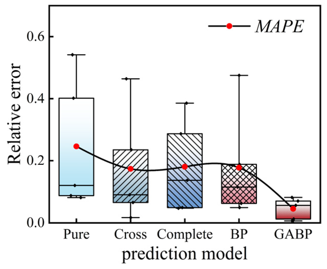
The relative error and MAPE of each type of prediction model are shown in Figure 9. Among them, the pure quadratic model had the worst prediction performance, and its prediction accuracy was only 75.4%, while the cross model and the complete quadratic model could be improved, and the prediction accuracy was around 82%. The prediction model established by the neural network efficiently narrowed down the error distribution range. However, it failed to effectively cut down the MAPE, and its prediction accuracy stood at 82.2%. The neural network coupled with GA improved the prediction accuracy by 95.5% on the basis of reducing the error distribution. Comprehensive analysis indicated that the relative prediction error of the neural network integrated with the GA was much closer to zero. For each sample, the predicted values were nearer to the actual values, demonstrating a higher prediction accuracy.

Figure 9.
Distribution of prediction error.
In addition, the mean absolute error (MAE), mean square error (MSE), and root mean square error (RMSE) were calculated and compared in order to comprehensively compare the prediction ability of the two neural networks. The calculation formulae were as follows:
The prediction errors of the prediction models are shown in Table 5. The errors of the mathematical regression prediction model were large. The prediction model constructed by the neural network effectively reduced MAE, MSE, and RMSE, reaching 0.459, 0.311, and 0.557, respectively. After coupling GA, the various errors were further reduced, and MAE, MSE, and RMSE were reduced to 0.138, 0.032, and 0.179, respectively. A comprehensive analysis revealed that the neural network prediction model outperformed the traditional mathematical regression prediction model in terms of prediction performance. Moreover, coupling with GA further reduced the errors of the neural network, enhancing its performance, and efficiently preventing the network from getting trapped in local minimum values during the training process.
Table 5.
Prediction error statistics of MRR.
5. Conclusions
In this paper, orthogonal experiments were performed on TC4 titanium alloy specimens treated by vertical vibratory finishing. Through variance analysis, the impacts of the vibration frequency, the phase difference of the eccentric block, the mass of upper eccentric block, and the mass of lower eccentric block on the MRR were investigated. An MRR prediction model was established using mathematical regression and a neural network. Moreover, the neural network was optimized by the genetic algorithm. After a comparative analysis, the following conclusions can be drawn:
- (1)
- Through theoretical analysis and variance analysis of orthogonal experiment results, it can be concluded that vibration frequency had the greatest influence on the MRR, and the corresponding F value was 3.372. This was followed by the eccentric block phase difference, corresponding to an F value of 2.033. The influence of the mass of the lower eccentric block and the mass of the upper eccentric block on the material removal rate were small and close, and the corresponding F values were 1.416 and 1.112, respectively.
- (2)
- The prediction model of the MRR was constructed according to the experimental data. In the mathematical regression model, the prediction accuracy of the cross-over model and the complete quadratic model for the verification set hovered around 82%. However, the maximum error reached 2.563. The prediction accuracy of the neural network attained 82.2%; meanwhile, its maximum error decreased to 1.039. Through comparison, it can be clearly seen that the neural network exhibited a superior prediction effect.
- (3)
- The neural network prediction model constructed by coupled GA reduced the error distribution range, reducing the MAPE from 0.178 to 0.045, and increasing the prediction accuracy to 95.5%. The constructed MRR prediction model had the best prediction performance and the highest accuracy, which verified the application of the GABP neural network in vertical vibratory finishing, and provided a new method for the control of process parameters in vibratory finishing.
This paper takes the MRR as an example to build a prediction model of vertical vibratory finishing. Our model obtained a high prediction accuracy and realized the prediction of the MRR of TC4 material processed by ZK-60 vertical vibratory finishing equipment. At present, the prediction model is only in the research and development stage; there are still many surface quality evaluation indexes (such as surface roughness) that have not been established. In the future, on the basis of this, further research will be carried out in the field of vertical vibratory finishing technology to carry out research on actual processing problems, verify the adaptability, and improve the prediction model.
Author Contributions
Conceptualization, K.S.; data curation, K.S., L.Z. and X.W.; formal analysis, K.S. and L.Z.; funding acquisition, W.L. and X.L.; investigation, L.Z., B.T., Y.Z. and W.L.; methodology, K.S. and W.L.; software, K.S. and X.W.; validation, L.Z., B.T., Y.Z., W.L., X.L. and X.W.; writing—original draft, K.S. and L.Z.; writing—review and editing, W.L. and X.L. All authors have read and agreed to the published version of the manuscript.
Funding
The work was co-supported by the National Natural Science Foundation of China (Grant Nos. 51875389, 51975399, and 52075362) and the Central Government Guides Local Foundation for Science and Technology Development (Grant Nos. YDZJSX2022A020 and YDZJSX2022B004).
Institutional Review Board Statement
Not applicable.
Informed Consent Statement
Not applicable.
Data Availability Statement
Data will be made available on request.
Conflicts of Interest
Authors Kun Shan and Yashuang Zhang were employed by the company AECC Shenyang Liming Aero-Engine Co., Ltd. Author Bo Tan was employed by the company AECC South Industry Company Limited. The remaining authors declare that the research was conducted in the absence of any commercial or financial relationships that could be construed as a potential conflict of interest.
References
- Bu, J.; Gao, Z.; Niu, J.; Cao, Y. Crack Failure Analysis of a Fan Stator Vane. Aeroengine 2021, 47, 91–95. [Google Scholar]
- Yang, S.; Wang, X.; Li, W. Research Status and Further Development of Vibratory Finishing Technology. J. Taiyuan Univ. Technol. 2017, 48, 385–392. [Google Scholar]
- Mediratta, R.; Ahluwalia, K.; Yeo, S. State-of-the-art on vibratory finishing in the aviation industry: An industrial and academic perspective. Int. J. Adv. Manuf. Technol. 2016, 85, 415–429. [Google Scholar] [CrossRef]
- Wong, B.; Maiumdar, K.; Ahluwalia, K.; Yeo, S. Effects of high frequency vibratory finishing of aerospace components. J. Mech. Sci. Technol. 2019, 33, 1809–1815. [Google Scholar] [CrossRef]
- Yang, S.; Li, W.; Chen, H. Surface Finishing Theory and New Technology; National Defense Industry Press: Beijing, China, 2011. [Google Scholar]
- Li, H.; Zhao, Z.; Zhen, C.; Ji, Z.; Zhao, G. Effect of Laser Shock Finishing on the Surface Quality of 2024 Aluminum Alloy with Milled Plane. Surf. Technol. 2023, 52, 388–396. [Google Scholar]
- Wang, J.; Shi, H.; Gao, Z.; Li, X.; Li, W. The Effect of the Physical Properties of the Granular Media on the Finishing of 7075 Aluminum Alloy. Surf. Technol. 2021, 50, 358–366. [Google Scholar]
- Hao, Z.; Li, W.; Li, X.; Wu, F.; Zhao, W. Effect of media parameters on contact forces in centrifugal barrel finishing. China Sci. 2017, 12, 2756–2760. [Google Scholar]
- Maciel, L.S.; Spelt, J.K. Influence of process parameters on average particle speeds in a vibratory finisher. Granul. Matter 2018, 20, 65. [Google Scholar] [CrossRef]
- Zhang, C.; Liu, W.; Wang, S.; Liu, Z.; Morgan, M.; Liu, X. Dynamic modeling and trajectory measurement on vibratory finishing. Int. J. Adv. Manuf. Technol. 2020, 106, 253–263. [Google Scholar] [CrossRef]
- Tian, Y.; Zhong, Z.; Tan, S. Kinematic analysis and experimental investigation on vibratory finishing. Int. J. Adv. Manuf. Technol. 2016, 86, 3113–3121. [Google Scholar] [CrossRef]
- Hashemnia, K.; Mohajerani, A.; Spelt, J.K. Development of a laser displacement probe to measure particle impact velocities in vibrationally fluidized granular flows. Powder Technol. 2013, 235, 940–952. [Google Scholar] [CrossRef]
- Wang, S.; Timsit, R.S.; Spelt, J.K. Experimental investigation of vibratory finishing of aluminum. Wear 2000, 243, 147–156. [Google Scholar] [CrossRef]
- Domblesky, J.; Evans, R.; Cariapa, V. Material removal model for vibratory finishing. Int. J. Prod. Res. 2004, 42, 1029–1041. [Google Scholar] [CrossRef]
- Maciel, L.; Spelt, J. Bulk mass flow in a vibratory finisher: Mechanisms and effect of process parameters. Granul. Matter 2018, 20, 57–70. [Google Scholar] [CrossRef]
- Hashemnia, K.; Spelt, J.K. Particle impact velocities in a vibrationally fluidized granular flow: Measurements and discrete element predictions. Chem. Eng. Sci. 2014, 109, 123–135. [Google Scholar] [CrossRef]
- Tang, L.; Ren, L.; Feng, X.; Zhao, J.; Zhu, Q. Multi-objective Parameter Optimization and Regression Analysis of EDM for SiC/Al Functionally Graded Materials. Electromachining Mould. 2018, 2, 8–13+38. [Google Scholar]
- Naeim, N.; Aboueleaz, M.; Elkaseer, A. Experimental Investigation of Surface Roughness and Material Removal Rate in Wire EDM of Stainless Steel 304. Materials 2023, 16, 1022. [Google Scholar] [CrossRef]
- Song, Z.; Lv, B.; Ke, M.; Yang, Y.B.; Shao, Q.; Yuan, J.L.; Nguyen, D.N. Removal Rate Model of Deterministic Shear Thickening Polishing Material Based on BP Neural Network. Surf. Technol. 2020, 49, 320–325, 357. [Google Scholar]
- Peng, B.; Yan, X.; Du, J. Surface Quality Prediction Based on BP and RBF Neural Networks. Surf. Technol. 2020, 49, 324–328, 337. [Google Scholar]
- Yan, Y.; Li, Z.; Yu, X.; Zhao, J. Research on Measurement Method of Grinding Surface Roughness for Small Samples. Mach. Tool Hydraul. 2023, 51, 1–8. [Google Scholar]
- Tang, S.; Hakim, N.; Khaksar, W. Artificial Neural Network (ANN) Approach for Predicting Friction Coefficient of Roller Burnishing AL6061. Int. J. Mach. Learn. Comput. 2012, 2, 825–830. [Google Scholar] [CrossRef]
- Nguyen, T.; Nguyen, T.; Trinh, Q.; Le, X.B.; Pham, L.H.; Le, X.H. Artificial neural network-based optimization of operating parameters for minimum quantity lubrication-assisted burnishing process in terms of surface characteristics. Neural Comput. Appl. 2022, 34, 7005–7031. [Google Scholar] [CrossRef]
- Kanovic, Z.; Vukelic, D.; el Simunovic, K. The Modelling of Surface Roughness after the Ball Burnishing Process with a High-Stiffness Tool by Using Regression Analysis, Artificial Neural Networks, and Support Vector Regression. Metals 2022, 12, 320. [Google Scholar] [CrossRef]
- Harlal, S.; Alakesh, M. Simulation of surface generated during abrasive flow finishing of Al/SiC_p-MMC using neural networks. Int. J. Adv. Manuf. Technol. 2012, 61, 1263–1268. [Google Scholar]
- Xu, L.; Chen, Y.; Han, B.; Chen, H.; Liu, W. Research on Surface Roughness Prediction Method of Magnetic Abrasive Finishing Based on Evolutionary Neural Network. Surf. Technol. 2021, 50, 94–100, 118. [Google Scholar]
- Ahamd, S.; Singari, R.; Mishra, R. Modelling and optimisation of magnetic abrasive finishing process based on a non-orthogonal array with ANN-GA approach. Trans. Inst. Met. Finish. Int. J. Surf. Eng. Coat. 2020, 98, 186–198. [Google Scholar] [CrossRef]
- Ahamd, S.; Singari, R.; Mishra, R. Tri-objective constrained optimization of pulsating DC sourced magnetic abrasive finishing process parameters using artificial neural network and genetic algorithm. Mater. Manuf. Process. 2021, 36, 843–857. [Google Scholar] [CrossRef]
- Wang, J.; Li, X.; Li, W.; Yang, S. Research of horizontal vibratory finishing for aero-engine blade movement characteristics and action behavior of media. Int. J. Adv. Manuf. Technol. 2023, 126, 2065–2081. [Google Scholar] [CrossRef]
- Wang, N.; Yang, S.; Cao, B.; Zhao, K. Influence of Different Machining Parameters of the Spindle Type Barrel Finishing on Surface Finishing Effect. Mach. Des. Manuf. 2020, 5, 206–209+213. [Google Scholar]
- Huai, C.; Huang, T.; Jia, X. Optimization of Processing Parameters in Grinding and Polishing Coupling Neural Networks with Genetic Algorithms. Mech. Sci. Technol. Aerosp. Eng. 2021, 40, 1025–1030. [Google Scholar]
- Liu, S.; Yi, J.; Xie, H. Research on quality prediction of surface polishing on die and mould parts based on improved BP algorithm. Mould Ind. 2023, 49, 9–19. [Google Scholar]
- Wang, Z.; Qin, K.; Ying, D. Prediction of heavy duty diesal vehicle emission based on GA-BP neural network with double hidden layer. J. Hefei Univ. Technol. (Nat. Sci.) 2019, 42, 735–740. [Google Scholar]
- Pang, C.; Jiang, Y.; Wu, T.; Liao, C.; Ma, W. Effect of Neural Network Parameters on Earthquake Type Recognition. Sci. Technol. Eng. 2022, 22, 7765–7772. [Google Scholar]

Disclaimer/Publisher’s Note: The statements, opinions and data contained in all publications are solely those of the individual author(s) and contributor(s) and not of MDPI and/or the editor(s). MDPI and/or the editor(s) disclaim responsibility for any injury to people or property resulting from any ideas, methods, instructions or products referred to in the content. |
© 2025 by the authors. Licensee MDPI, Basel, Switzerland. This article is an open access article distributed under the terms and conditions of the Creative Commons Attribution (CC BY) license (https://creativecommons.org/licenses/by/4.0/).