Abstract
In thermal spraying processes, molten, semi-molten, or solid particles, which are sufficiently fast in a stream of gas, are deposited on a substrate. These particles can plastically deform while impacting on the substrate, which results in the formation of well-adhered and dense coatings. Clearly, particles in flight conditions, such as velocity, trajectory, temperature, and melting state, have enormous influence on the coating properties and should be well understood to control and improve the coating quality. The focus of this study is on the high velocity oxygen fuel (HVOF) spraying and high velocity suspension flame spraying (HVSFS) techniques, which are widely used in academia and industry to generate different types of coatings. Extensive numerical and experimental studies were carried out and are still in progress to estimate the particle in-flight behavior in thermal spray processes. In this review paper, the fundamental phenomena involved in the mentioned thermal spray techniques, such as shock diamonds, combustion, primary atomization, secondary atomization, etc., are discussed comprehensively. In addition, the basic aspects and emerging trends in simulation of thermal spray processes are reviewed. The numerical approaches such as Eulerian-Lagrangian and volume of fluid along with their advantages and disadvantages are explained in detail. Furthermore, this article provides a detailed review on simulation studies published to date.
1. Introduction
Thermal spraying is a process in which molten, semi-molten, or solid particles are deposited on a substrate. Various thermal spray techniques such as atmospheric plasma spraying (APS), high velocity oxygen fuel spraying (HVOF), and cold spraying are extensively used in industry to generate many different types of coatings such as thermal barrier, wear resistance, and corrosion resistance. As the coating particles are molten or solid and sufficiently fast in a stream of gas, they can plastically deform while impacting on the substrate, which results in coating production. Obviously, the particle temperature and melting state and its kinetic energy have enormous influence on the coating properties. Therefore, the temperature, trajectory, and velocity of these fine particles must be well controlled to generate repeatable and desirable coatings [1,2,3,4].
The first goal of this article is to review the HVOF thermal spray technique, its simulation methods, and the simulations results. The HVOF coatings have been widely applied in industries such as in coating piston rings and cylinder bores in the automotive industry, rolls and blades in the pulp and paper industry, ball and gate valves in the process industry, and the production of thermal barrier coatings for turbine sections and landing gears in the aerospace industry. The HVOF system is able to generate anti-corrosion protective coatings that are useful in the energy industry particularly to protect power plant boilers [4,5,6]. The main physical phenomena involved in the HVOF process and the available numerical approaches for its simulation are not discussed in detail in the previous review papers [4,5]. Therefore, the focus of this review is to explain these phenomena and the numerical methods comprehensively to prepare an all-inclusive document for simulation, design, and optimization of the HVOF torch. Various fields such as turbulent, multiphase, and compressible flows, combustion, and shock dynamics that are involved in the HVOF process are covered in this paper. Section 1.1 provides the summary of the HVOF process along with the explanation of the main physical phenomena involved in it, while Section 2 discusses the Eulerian-Lagrangian approach and prepares accurate empirical and theoretical formulas to simulate this process. Last of all, a review on the recent published HVOF modeling works is provided in Section 3. This review covers almost all published articles related to the modeling of the HVOF process.
Another goal of this article is to review the suspension thermal spray (STS) technique, especially the high velocity suspension flame spraying (HVSFS) technique. This technique is used to generate fine microstructured coatings. The fine microstructured coatings have attracted considerable attention due to various unique properties such as enhanced catalytic behavior, remarkable wear resistance, superior thermal insulation, and thermal shock resistance [7]. It will be revealed that many parameters and mechanisms in the suspension spraying technique are still unknowns and must be understood. In addition, it will be discussed that suspension thermal spray simulation is more difficult than the modeling of conventional thermal spray processes due to the presence of some physical phenomena such as atomization. Therefore, the fundamental phenomena involved in the STS process are discussed in Section 4 and a review on the HVSFS modeling works published to date is given in Section 5.
High-Velocity Oxygen-Fuel (HVOF) Thermal Spray Technique
In a typical HVOF process, fuel (gas or liquid) and oxygen are injected into the combustion chamber and ignited. Then the exhaust gas goes through a nozzle and a supersonic jet is obtained which emerges into the surrounding air (see Figure 1) [1]. The powder can be injected into the jet in radial or axial directions using a carrier gas which is usually nitrogen or argon [1]. The HVOF system can be used to spray metals, metallic alloys, cermets, ceramics, and polymers [1,4,6,8,9]. However, particles are usually composites with carbide reinforcements, metals, and alloys, and are in the range of 5–45 µm [1]. Recently, instead of powder injection, suspension, which is a combination of fine solid particles (usually in the range of 500 nm–5 µm) and a base fluid such as water or alcohol (e.g., ethanol), is injected into the jet using spray atomization or injection of continuous jet methods. This technique will be explained comprehensively later in this article. Due to the nozzle geometry, chamber pressure, and flame temperature, the particles in the HVOF process undergo high velocity (more than 500 m/s) and temperature in a way that their temperature reaches the melting point or above. The wire/rode is also applied in this technique to generate the molten particles. The ends of the wire/rode become molten in the flame and then atomized by compressed air to form droplets and these droplets accelerate toward the substrate. The distance between torch exit and the substrate in the case of dry powder injection is typically in the range of 150–300 mm [1]. It is revealed that in the case of suspension injection, the standoff distance should be less than that in the case of dry powder injection (around 100 mm). Water, air, or a mixture of both (hybrid) can be used for cooling the combustion chamber and the nozzle.
Figure 1.
Schematic of a typical HVOF nozzle. Adapted from Reference [8] with permission from the author.
Figure 1.
Schematic of a typical HVOF nozzle. Adapted from Reference [8] with permission from the author.
Combustion is the energy source of the HVOF system. The fuel can be hydrogen and hydrocarbon gases/liquids such as ethylene, propylene, propane, natural gas, and kerosene (the atomized liquid) [1]. The combustion chamber pressure is usually in the range of 0.3–1 MPa. Generally, oxygen and fuel are mixed before injection into the combustion chamber (premixed flame). The oxygen-fuel ratio and the fuel type have significant influences on the coating properties. For example, by using fuel-rich mixtures, metallic coatings with less oxide contents are produced. Since in-flight reactions are the main reason of the coating oxidation, the presence of less oxygen in the chamber causes the particles to oxidize less. Moreover, longer flames also decrease the oxidation level. Longer flames have two major effects: first, they can burn more oxygen and, second, they can shorten the particle interaction with the surrounding air [6].
The oxygen-fuel ratio is normally reported in terms of a non-dimensional variable called the equivalence ratio, which is defined as follows:
where m and n stand for the mass and the number of moles, respectively. For fuel-rich mixture ϕ > 1 and for fuel-lean mixture ϕ < 1. ϕ = 1 is defined as the stoichiometric condition. The adiabatic flame temperature as a function of the equivalence ratio for various fuel-air mixtures at standard condition for temperature and pressure (STP) is shown in Figure 2. It is clear from Figure 2 that the maximum flame temperature occurs near the stoichiometric condition ϕ = 1 or somewhat on the fuel-rich side [10]. The adiabatic flame temperature increases with the increase of the chamber pressure. The high pressure environment also has other important effects on the premixed flame such as a decrease of the turbulence scales, particularly the Kolmogorov scale, with the increase of the pressure [11,12,13,14]. Furthermore, as pressure increases, the wrinkled structures of the flames become very fine and complex, the cusps become sharp, the flamelet breaks at many points throughout the flame, and the scales of these broken flamelets become small. Moreover, the flame thickness decreases as the pressure increases. Consequently, the flame in the combustion chamber of the HVOF system is turbulent.

Figure 2.
The adiabatic flame temperature as a function of the equivalence ratio for various fuel-air mixtures at STP. Reproduced from Reference [10] with permission (Copyright Cambridge University Press 2006).
Figure 2.
The adiabatic flame temperature as a function of the equivalence ratio for various fuel-air mixtures at STP. Reproduced from Reference [10] with permission (Copyright Cambridge University Press 2006).
The nozzle geometry can be the convergent barrel, the convergent-divergent nozzle (de Laval), or the convergent-divergent barrel [1]. Regarding nozzle geometry and combustion chamber pressure and temperature, a supersonic flow is obtained and shock diamonds are formed at the nozzle exit. It is known from the experiments that seven to nine shock diamonds are observable in a typical HVOF process. The classical gas dynamics theory predicts shock waves, Prandtle-Meyer fans (expansion and compression fans), and slip lines [15,16,17]. For smoothly contoured convergent-divergent (C-D or de Laval) nozzles, the presence of shock diamonds means that the Mach number at the nozzle exit is higher than 1 and there is a supersonic jet. A supersonic jet is referred to as underexpanded if Pe/Pa > 1, overexpanded if Pe/Pa < 1, and fully expanded (free of shock diamonds) if Pe/Pa = 1, where Pe is the gas pressure at the nozzle exit and Pa is the ambient gas pressure [15,16,17]. For a convergent nozzle, the existence of shock diamonds means that the Mach number at the nozzle exit is equal to 1 and the pressure at the nozzle exit is higher than the ambient pressure. Therefore, the jet is underexpanded. The underexpanded and overexpanded supersonic jets are shown in detail in Figure 3 and Figure 4, respectively [17].
Figure 3.
The underexpanded supersonic jet [17].
Figure 3.
The underexpanded supersonic jet [17].
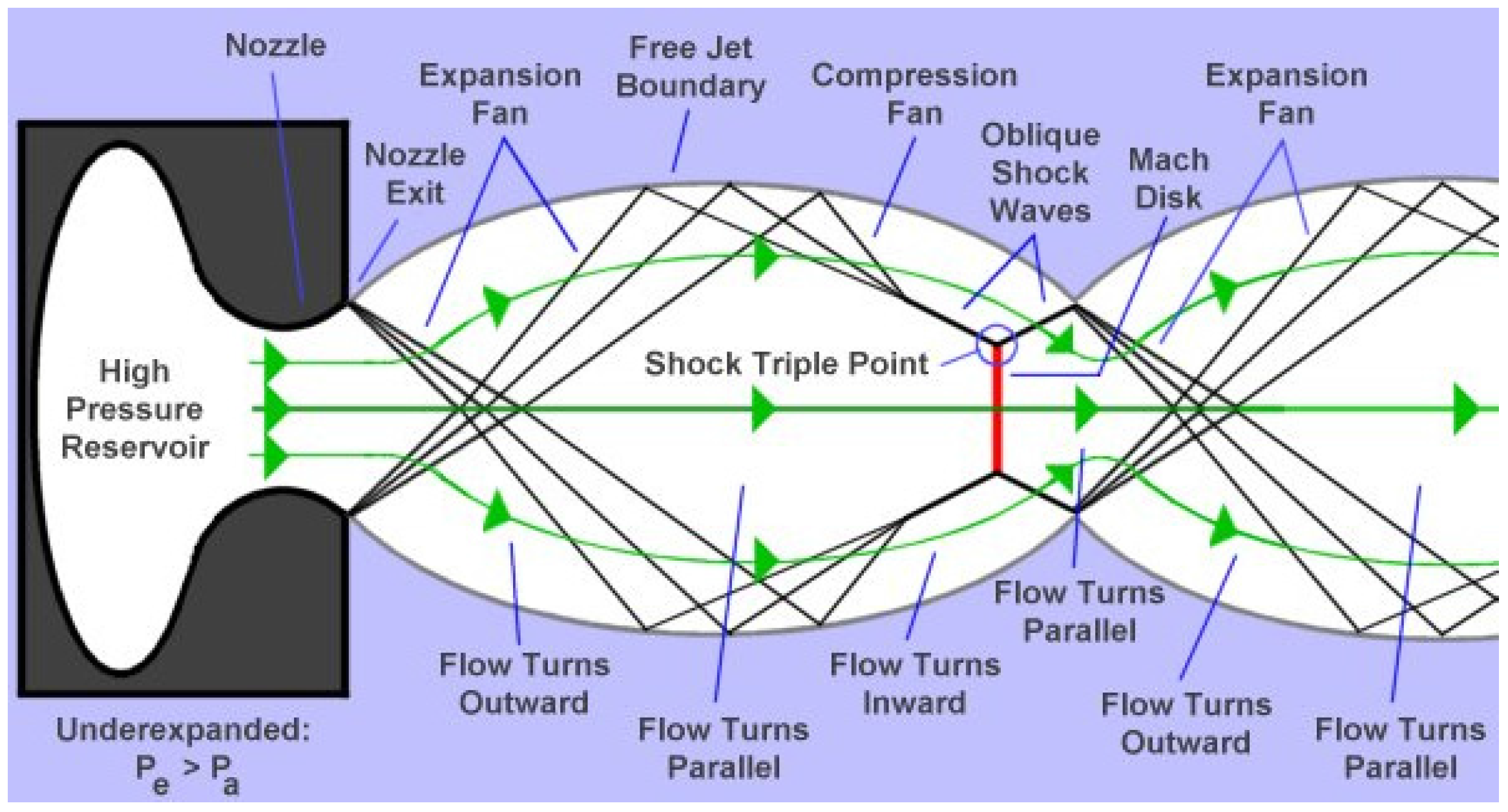
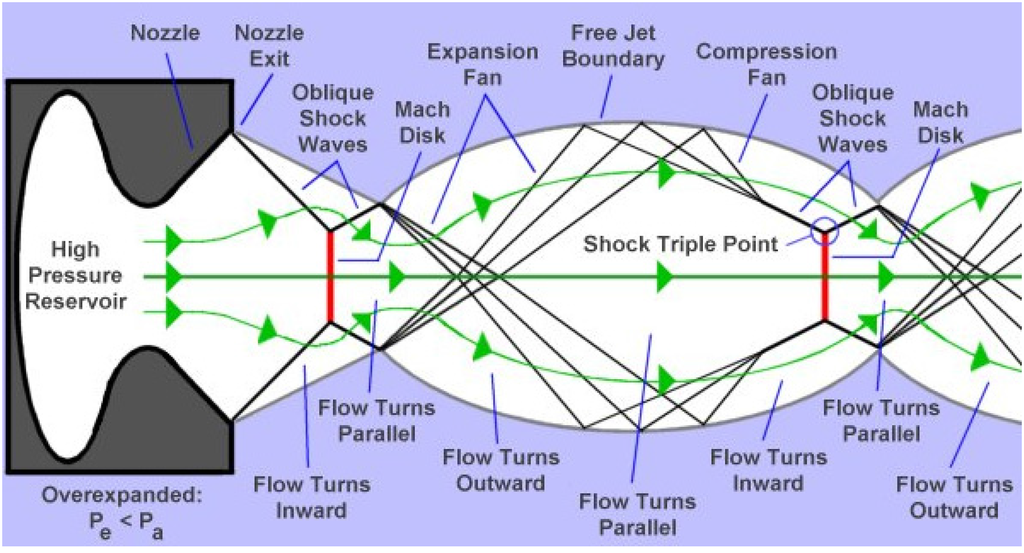
Figure 4.
The overexpanded supersonic jet [17].
Figure 4.
The overexpanded supersonic jet [17].
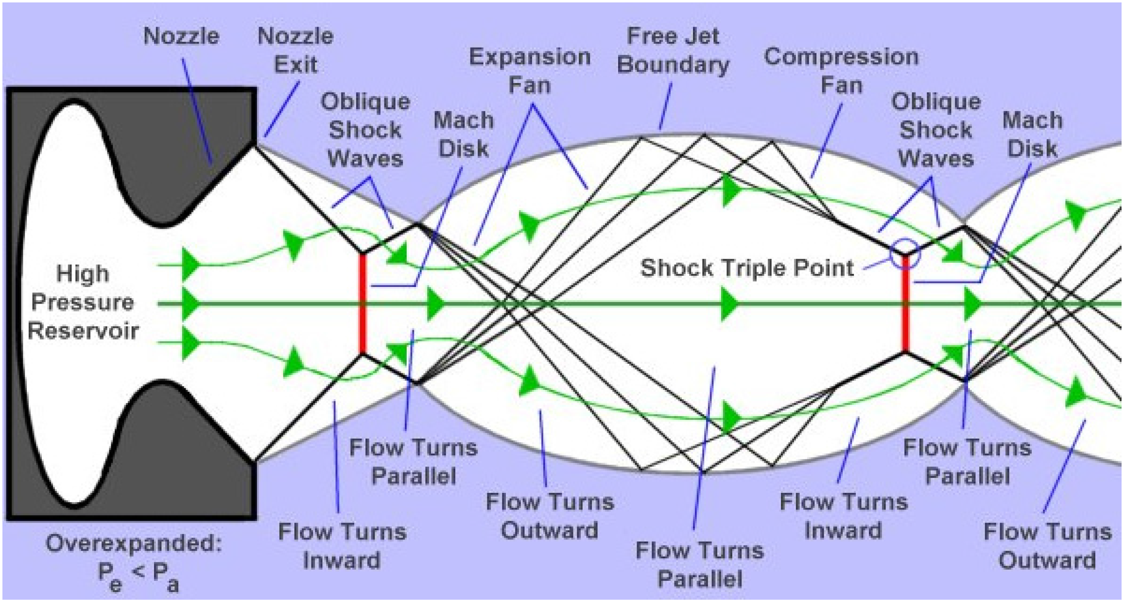
In the underexpanded condition, the expansion fans exist at the nozzle exit, and in the overexpanded condition, the shock waves occur at the nozzle exit. When the flow goes through the expansion fans, its pressure decreases and its velocity increases, and when it goes through the shock waves, its pressure and velocity increase and decrease, respectively. The boundary between the supersonic jet and the surrounding gas is a slip line (also called free jet boundary) [15,16,17]. The slip lines separate the regions with the same pressures but with different densities and temperatures. Noting that, no gas flows across these lines. Therefore, the gas tangential velocity on one side of the slip line is different from the gas tangential velocity on the other side. When a shock wave incidents on a slip line, it reflects as expansion fans and when expansion fans incident on a slip line, they reflect as compression fans which merge into an oblique shock wave [15,16,17]. The slip line turns outward because of the incident shock and the reflected expansion fans’ effects. Conversely, the slip line turns inward because of the incident expansion fans’ and reflected compression fans’ effects [15,16,17]. When Pe << Pa or Pe >> Pa, the strong normal shocks called Mach disks exist in the flow. It is clear that the incident shock reflects at the Mach disk perimeter and makes a shock triple point. In a real supersonic jet, the turbulent mixing layer grows until it reaches the jet axis and after this point the flow is subsonic and fully turbulent [15].
It should be considered that the above discussion is only applicable for the nozzle with a smooth and large-radius curve throat. The nozzle geometry plays a significant role on the structure of the supersonic jets and can change the above discussion. For example, consider a conical convergent-divergent nozzle (CCD) with a relatively sharp corner at the throat. It has been revealed that due to the sharp corner of the throat, there might be oblique shocks and a Mach disk inside the divergent part of the nozzle. These oblique shocks and Mach disk do not depend on the condition outside the nozzle and can change the supersonic jet regime and shock diamond pattern at the nozzle exit (a double-diamond pattern may occur at the nozzle exit) [18,19].
The shocks have some influence on the gas turbulence. Generally, the main result of the shock-turbulence interaction is the amplification of the velocity fluctuations (turbulence amplification) [20,21]. As a simple example, consider the shock interaction with the isotropic homogeneous turbulence [20,21]. In this case, an amplification of longitudinal velocity fluctuations is observed through the interaction while the fluctuations of the other two components are slightly reduced or remain unaffected [20]. As a result, the flow downstream of the shock is anisotropic [21]. It should be noted that the shock properties (e.g., the shock strength, angle, location, and shape), the incoming flow turbulence condition, the incoming flow compressibility degree, and the geometry have influence on the shock-turbulence interaction outcomes [20,21].
It is proved that particles can affect the mixture sound speed and chocking condition. By considering the gas-particle mixture as a single pseudo-homogeneous phase [22,23,24,25] and using the classical gas dynamics theory [26], it is obtained that the ratio of the mixture sound speed, am, to the pure gas, ag, is a function of the particle mass fraction ϕ and the particle properties such as density, ρp, and specific heat capacity, c, (see Figure 5) [22,23]. As it is clearly demonstrated in Figure 5, for dilute flow am < ag and when the particle mass fraction increases, the mixture sound speed decreases [22,23]. However, when the amount of the particle mass fraction ϕ is too high, some of the assumptions in classical gas dynamics are not applicable and the results shown in Figure 5 cannot be acceptable anymore [23]. Moreover, Figure 5 shows the effect of particle-specific heat capacity on the mixture sound speed. As the particle-specific heat capacity increases, the sound speed of the mixture decreases. In this figure the ratio of the gas phase density to the particle density is assumed to be ρ/ρp = 0.01, noting that variation of this ratio can change the mixture sound speed.
It is known that the shocks have significant influences on the particle behavior [22]. A typical and simple way to study the shock-particle interaction is to assume a normal shock wave which is moving in a stationary gas-particle mixture. Similar to the moving shock analysis in the classical gas dynamics theory [26], the coordinates are attached to the shock wave so that the shock wave becomes stationary and the mixture is moving. Based on the velocities and temperatures of the particle (up, Tp) and the gas (u, T) phases, three different zones are defined and shown in Figure 6 as the equilibrium zone in front of the shock wave (subscript 1), the transient zone behind the shock wave (subscript 2), and the equilibrium zone far away behind the shock wave (subscript ∞) [22,23,24,25]. In the transient region, the particle and the gas velocities and also their temperatures are different because the particle needs time to respond to the momentum and heat changes and to reach a new equilibrium condition. The presence of the transient zone for the particle phase can somehow describe the reason of the particle trajectory deviation in the shock diamonds of the HVOF nozzles. In other words, as there are many shock waves and expansion fans behind each other in the shock diamonds of the HVOF system, the particle (especially fine particles) trajectory is severely influenced by them. It should be noted that immediately after each shock the gas temperature and pressure increase significantly while the velocity reduces considerably. Hence, the heat transfer rate from the gas phase to the particles increases in this region. As a result, the shock diamonds should be captured precisely in order to predict the particle temperature, velocity, and trajectory accurately.
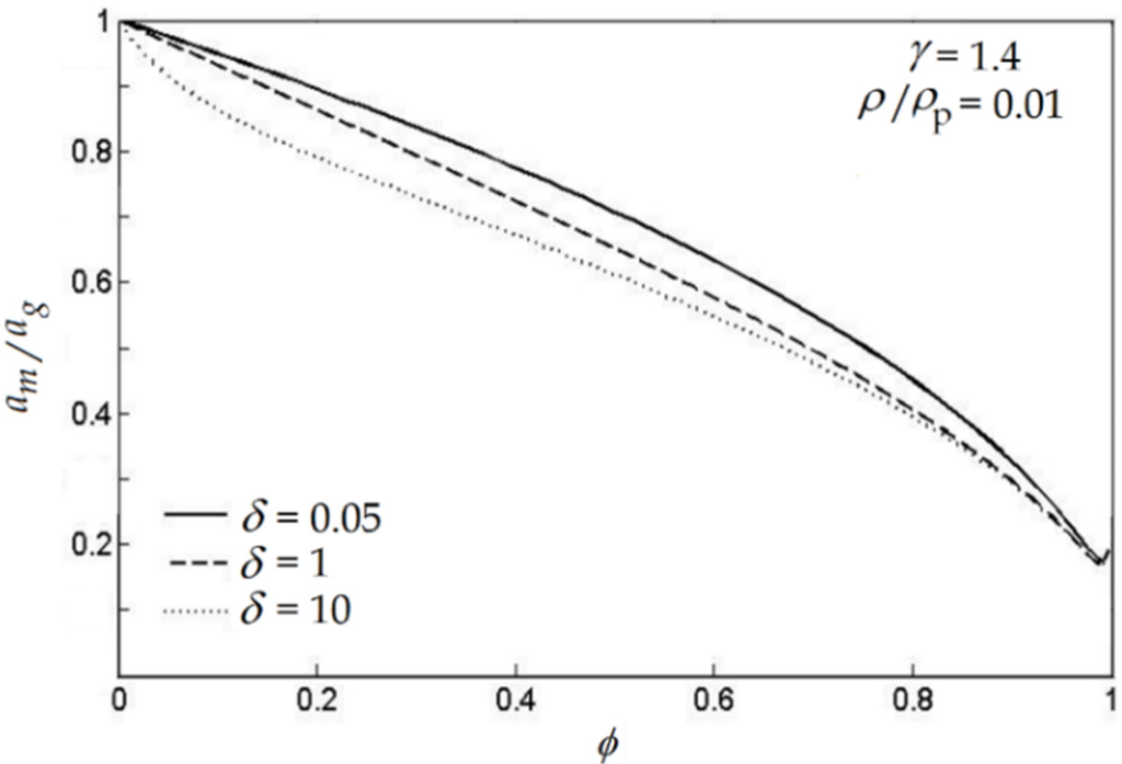
Figure 5.
The ratio of sound speed of mixture to gas (am/ag) as a function of particle mass fraction ϕ and particle density and specific heat capacity (ρp, c). Thus, δ = C/Cp, γ = Cp/Cv and Cp, Cv are the specific heat capacities of the gas phase [23].
Figure 5.
The ratio of sound speed of mixture to gas (am/ag) as a function of particle mass fraction ϕ and particle density and specific heat capacity (ρp, c). Thus, δ = C/Cp, γ = Cp/Cv and Cp, Cv are the specific heat capacities of the gas phase [23].
Figure 6.
The distribution of velocities (a) and temperatures (b) of the gas (u, T) and the particle (up, Tp) phases across the normal shock wave. Reproduced from Reference [22] with permission (Copyright Cambridge University Press 1998).
Figure 6.
The distribution of velocities (a) and temperatures (b) of the gas (u, T) and the particle (up, Tp) phases across the normal shock wave. Reproduced from Reference [22] with permission (Copyright Cambridge University Press 1998).
Based on the torch geometry and power level, the HVOF technique is divided into three generations [6]. The first generation of HVOF torches includes a relatively large combustion chamber with a straight nozzle or a convergent barrel which can produce, at most, the sonic speed at the gun exit. In the second generation, the nozzle geometry consists of a de-Laval nozzle so that the Mach number at the gun exit is higher than 1. The main difference between the first and second generations is the nozzle geometry. In the third generation, the combustion chamber pressure and the power level are increased; hence, the spraying rate is larger as well. Pursuing the HVOF technique generation by generation, the aim is to increase the gas pressure and the particle velocity and to decrease the flame and particle temperature [6]. Therefore, generation by generation, the coating density is enhanced because the oxidation amount in the coating is decreased and the flattening rate is grown.
From the above discussion, it is clear that the HVOF is a complex process that includes compressible turbulent multiphase flow with chemical reactions. However, simulation of this system and estimation of particle in-flight behavior are very crucial for industries and academia to improve the coatings’ properties. During the past 25 years, analytical and computational fluid dynamics (CFD) models have been widely used to simulate the HVOF process. Initially, some simple one-dimensional (1D) analytical models were developed. In these models, combustion, turbulence, and shock diamond modeling were ignored and simplifying assumptions were used to analyze the in-flight particle behavior. However, after developments of CFD codes, numerical methods are extensively used to simulate combustion, turbulence, and to capture shock diamonds in two-dimensional (2D) and three-dimensional (3D) computational domains and the in-flight particle behavior can now be modeled accurately. In this review paper, the results of both analytical and numerical models will be explained in detail.
2. Governing Equations
The flow of small droplets or solid particles in a gas has been broadly studied by scientists and engineers for years. Today, several numerical approaches are available to model the behavior of gas-particle/droplet flow, such as the Lagrangian trajectory approach (Eulerian-Lagrangian model), the Eulerian continuum approach (Eulerian-Eulerian model or two-fluid model), the kinetic theory, and the Ergun theory. In the Eulerian-Lagrangian approach, the gas is modeled as a continuum phase while Lagrangian trajectory models are used to simulate the particles’ motion and heat transfer. Lagrangian trajectory models can be categorized as stochastic and deterministic models. The stochastic model considers the effect of gas turbulence on the particle motion and heat transfer; however, the deterministic model neglects the gas turbulence effects. One-way coupled and two-way coupled are other assumptions used in this approach. In one-way coupled assumption, only the effect of one phase on the other is considered and there is no reverse effect. In other words, one-way coupled assumption is applied when, in a gas-particle mixture, the effect of the gas phase on the particle phase equations is considered and the effect of the particle phase on the gas phase equations is ignored. In two-way coupled assumption, the effects of both phases on each other are considered [22,27]. The Eulerian-Lagrangian approach is suitable for dilute flow modeling. In the Eulerian-Eulerian approach, all phases are assumed to be continuum and this method is suitable for dense flow modeling [28,29]. The kinetic theory is used when the concentration of the particles is high so that the interparticle collisions become the dominant transport mechanism. This method assumes the particle as a molecule. The Ergun theory calculates the pressure drop in a packed bed [22]. It should be noted that the Eulerian-Eulerian and the Eulerian-Lagrangian approaches are used to model the thermal spray processes because the concentration of the particle phase is not too high in these systems.
To choose the right model, dense and dilute flows should be defined. One way to explain dilute and dense flows is based on the dispersed phase influences on the gas phase turbulence [30]. If the dispersed phase volume fraction is less than 10−6, the dispersed phase has no influence on the turbulence of the gas phase. Therefore, the Eulerian-Lagrangian approach with one-way coupled assumption should be applied. However, if the dispersed phase volume fraction is between 10−6 and 10−3, the presence of dispersed phase influences the gas phase turbulence. Hence, the Eulerian-Lagrangian approach with two-way coupled assumption should be used. For volume fractions over 10−3, the existence of dispersed phase affects the gas phase turbulence more and particle-particle interactions play a significant role. The flow that has these properties is typically named dense flow. The Eulerian-Eulerian approach is necessary to model dense flow. The gas-particle flow regimes as a function of the dispersed phase volume fraction and the Stokes number is shown in Figure 7 [30]. The Eulerian-Lagrangian approach, which is focused on in this paper, is used to model the thermal spray processes extensively. However, the Eulerian-Eulerian approach was only used by Dolatabadi et al. and Samareh et al. [31,32] to model the dense flow in HVOF and cold spray nozzles. Since this approach is not usually used to model the thermal spray processes, it is not covered in this paper and the interested reader is referred to references [28,29,31,32] for further information.
Figure 7.
The gas-particle flow regimes as a function of the particle phase volume fraction and the Stokes number. Adapted from Reference [30] with permission (Copyright Springer 1994).
Figure 7.
The gas-particle flow regimes as a function of the particle phase volume fraction and the Stokes number. Adapted from Reference [30] with permission (Copyright Springer 1994).

As mentioned above, in the Eulerian-Lagrangian approach, the particle phase is simulated by Lagrangian trajectory models while the gas phase is modeled as a continuum phase. The forces which control the motion of the particles are fluid-particle, particle-particle interaction forces, and external fields’ forces. The main fluid-particle forces are drag, Basset, carried mass (virtual mass), buoyancy, thermophoresis, Saffman, and Magnus forces [22,27]. The key particle-particle forces are Van der Waals, electrostatic, and collision forces. Finally, the chief external fields’ forces are gravitational, electric, and magnetic forces [22,27]. Generally, the most important forces acting on a particle in thermal spray processes are drag and thermophoresis. The steady-state drag force is as follows
where CD, ρc, A, u, and v, are the drag coefficient, the carrier gas density, the particle projected area, the gas phase, and the particle velocity, respectively. As shown in Figure 8, CD is a function of Reynolds (Re) and Mach (M) numbers. In general, when the Reynolds number is high, the drag coefficient increases with the Mach number. (It should be mentioned that Figure 8 shows the approximate values of CD. In reality, for a high Reynolds flow, CD reaches a maximum point for slightly supersonic flow. Then it slightly decreases and reaches a plateau. However, this phenomenon is negligible). The main reason of this phenomenon is the shock wave formation on the particle and the attendant wave drag [27].
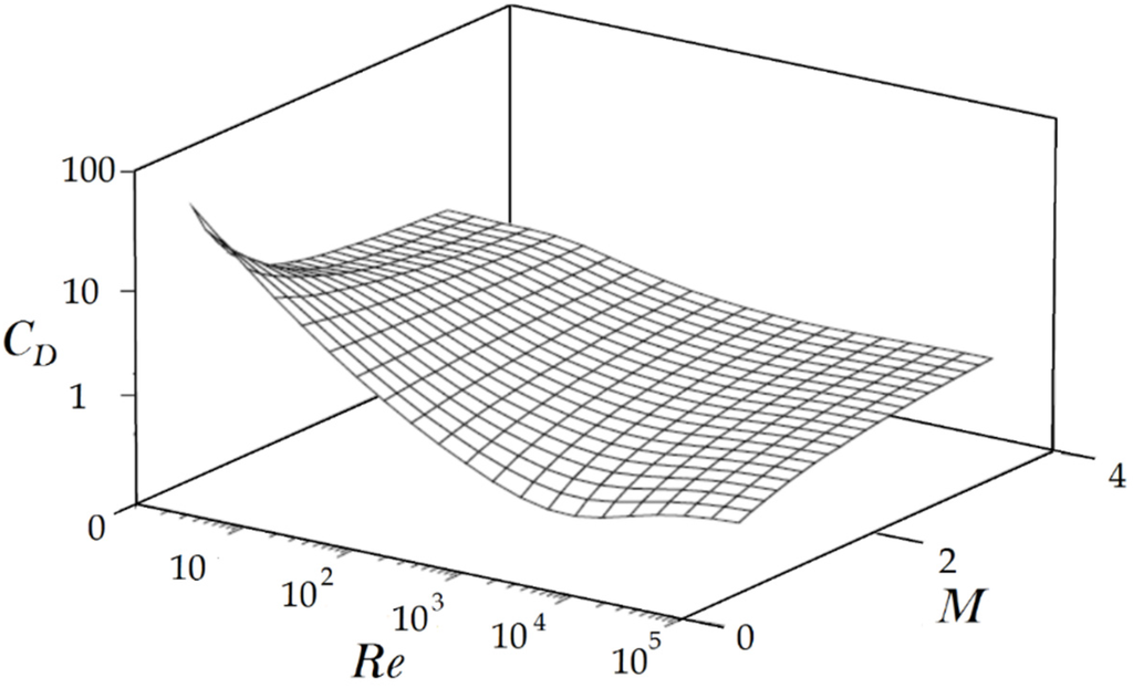
Figure 8.
The approximation of spherical particle drag coefficient as a function of the Mach number and Reynolds number. Reproduced from Reference [27] with permission (Copyright CRC Press 1998).
Figure 8.
The approximation of spherical particle drag coefficient as a function of the Mach number and Reynolds number. Reproduced from Reference [27] with permission (Copyright CRC Press 1998).

When the Reynolds number is low, as the Mach number grows, CD consistently reduces. In this case, rarefied effects (Knudsen number) play a significant role. The Knudsen number, which is defined as the ratio of the molecules mean free path λ to the diameter of the particle, Kn = λ/dp, is used to show the flow regimes. In general, when Kn < 10–3, the continuum assumption is correct. Moreover, when 10–3 < Kn < 0.25, the flow is known as slip flow where temperature jump and slip velocity exist between fluid and particle surface. When the Knudsen number is larger than 0.25, the molecular dynamics theory should be applied to simulate the particle behavior [27]. The following empirical correlation presented by Crowe [33] considers the effect of Mach, Reynolds, and Knudsen (it is proved that Kn ~ M/Re) numbers on the drag coefficient
where γ is the ratio of the specific heats and CD0 is the drag coefficient of a particle in an incompressible flow (where M ≈ 0) [34]. Furthermore, g(Re) and h(M) are as follows
where Td and Tc are the particle and carrier gas temperature, respectively. The above empirical correlation is only valid for Reynolds numbers less than the critical Reynolds number. At the critical Reynolds number, the boundary layer becomes turbulent and a sudden decrease in the drag coefficient occurs. However, this range is sufficient to model the particle dynamics in typical thermal spray processes [35]. It should be noted that the gas phase turbulence influences the drag coefficient and it causes the critical Reynolds number to decrease. Moreover, blowing (mass transfer) from a burning or evaporating droplet results in decrease of the drag coefficient [27]. More information regarding the mentioned phenomena can be found in reference [27].
The thermophoretic force sometimes plays a significant role in particle dynamics. The temperature gradient in the gas phase is the main reason of this force. As a higher temperature on one side of a particle results in higher molecular speeds, due to momentum exchange, a force is produced in the direction of decreasing temperature [27]. To model the thermophoretic force, the following empirical relation has been used extensively
where kc and kd are the gas and the particle thermal conductivities, respectively, md is the particle mass, d is the particle diameter, T is the gas temperature, ρc is the gas density, and μc is the gas viscosity. Cs, Cm and Ct are 1.17, 1.14, and 2.18, respectively [27]. The above correlation is acceptable for a wide range of thermal conductivity ratios and Knudsen numbers.
If the particle is homogenous and the Biot number (hd/kd) is less than 0.1, the lumped capacity method can be used to model the particle heat transfer
where Cd is the particle phase specific heat, h is the heat transfer coefficient, and S is the particle surface area. The Nusselt number (Nu) is used to calculate the heat transfer coefficient and is usually estimated by the Ranz-Marshal equation
where Pr is the Prandtl number of the gas phase [22,27]. In general, the Nusselt number decreases for rarefied flows. To consider the effect of the Knudsen number, the following correlation is suggested
where Nu0 is the Nusselt number for an incompressible flow [27]. It should be noted that since the blowing effects or mass transfer from a burning or evaporating droplet lower the gas phase temperature gradient at the droplet surface, the Nusselt number reduces [27].
The radiation heat transfer is usually ignored in the HVOF simulation. However, the simplest way to model the radiation heat transfer effects on the particle phase is to assume a diffuse-gray surface. In this case, the absorptivity, α, and the emissivity, ε, are independent of radiation direction and wavelength, and depend on temperature only [36]. From Kirchhoff’s law ε = α, therefore, the particle heat transfer equation becomes
where σb = 5.6704 × 10⁻⁸ W/(m2·K4) is the Stefan-Boltzmann constant, and T∞ is the ambient temperature. It should be noted that the ratio of the convection heat transfer to the radiation heat transfer for particle phase in the HVOF process is around 100 [37]. A more accurate way to model the radiation heat transfer is to consider the gas-particle mixture as a translucent media capable of emitting, absorption, and scattering radiation. Thus, the radiation heat transfer effect on both gas and particle phases can be modeled. Consider radiation of intensity iλ(x) along a path x within an absorbing, emitting, and scattering medium. The following equation (which is known as the radiation transfer equation) shows the change in the radiation intensity with distance x in the solid angle dω around the specific direction
where aλ, σsλ are the absorption and scattering coefficients, correspondingly, iλb is the blackbody intensity, and Φλ(ω, ωi) is the phase function. The terms on the right-hand side of the equation are related to the loss by absorption, gain by emission, loss by scattering, and gain by scattering into x direction, respectively. Generally, the absorption and the scattering coefficients are strongly dependent on the particle phase properties such as particle number density, size, shape, and material. Solving Equation (9) is difficult due to its integro-differential form. However, it is proved that for dilute mixtures the integral term is negligible [22]. Obviously, it is beyond the scope of this paper to describe the above equation in detail. For more information see references [36,37,38,39,40,41,42,43,44,45].
As mentioned before, in the Eulerian-Lagrangian method, the gas phase is modeled as a continuum. The compressible form of the mass, momentum, species mass fractions (Yk), and internal energy equations of the gas phase are as follows [46]:
Continuity
Momentum
Species continuity (k = 1,…,N)
Energy
where ρ, P, u, q, and τ are gas density, pressure, velocity vector, heat flux, and viscous shear stress, respectively. e stands for the mixture internal energy (, where hk is the enthalpy of the kth species), fk stands for the body force related to the kth species. and Vk stand for the kth species reaction rate, and the diffusive speed of the kth species, respectively. For a Newtonian fluid, the tensor of viscous shear stress is given by
where I, μ, γ are the identity matrix, the dynamic, and the bulk viscosity, respectively. The transport of species is represented by the bulk flow, ρu.∇Yk, and the diffusion phenomenon, ρYkVk. The Fick’s law model is usually used to evaluate the diffusive speed of the kth species. In this model Vk is related to the molar (Xk) or mass fraction gradients as follows
where stands for the coefficient of mixture-averaged mass diffusion (mixture-averaged diffusivity) for species k. If the ratio of diffusion coefficients is constant (e.g., constant Lewis number or Schmidt number), is explained as follows
where Lek, λ, and cp are the Lewis number of kth species, the mixture thermal conductivity, and the mixture specific heat, respectively [46]. The heat flux term q includes heat conduction, thermal radiation, and the effect of heat diffusion by mass diffusion of the various species [46]
There are several models to simulate the reaction rate term, , such as the laminar finite rate model, the eddy dissipation model (EDM), and the finite-rate/eddy-dissipation models [47], that are broadly considered as the combustion models in the HVOF simulation. The laminar finite rate model is suitable for laminar flames and inexact for turbulent flames. This model uses the Arrhenius expressions and the mass action law to model the reaction rate term and ignores the turbulence fluctuation effects on the reaction [48]. For more information about the Arrhenius equation and the mass action law, see chemical kinetics chapters in combustion books [48,49]. As mentioned earlier, the flow inside the combustion chamber of the HVOF system is turbulent. Therefore, using the laminar finite rate model to simulate the HVOF system is not admired today. The eddy dissipation model is known as a turbulent-chemistry interaction model and is suitable for fast-burning fuels. The chemical kinetics rates are neglected and the overall reaction rate is controlled by the turbulent mixing. In this model, the burning process initiates without involving an ignition source, which is usually suitable for the diffusion (non-premixed) flames. However, for premixed flames, as soon as the reactants come into the computational domain the burning process initiates. A simple way to solve this problem is to calculate both the Arrhenius and the eddy-dissipation reaction rates, choosing the minimum of these two rates as the net reaction rate. This method is known as the finite-rate/eddy-dissipation model [47]. Both eddy-dissipation and finite-rate/eddy-dissipation models have been used to simulate the HVOF process and produced acceptable results.
A state equation such as ideal gas law is used to close the equations [46]
where Wk is the molecular weight of species k and Ru is the universal gas constant.
Three different computational approaches named direct numerical simulation (DNS), large eddy simulation (LES), and Reynolds-averaged Navier-Stokes (RANS) are available to solve the above equations. DNS produces the exact solution of the above equations so that all temporal and spatial scales of the turbulence are resolved. To attain this goal, the computational domains consisting of millions or higher number of grid points should be used [46]. Obviously, today it is not possible to use DNS for modeling of the gas-particle/droplet flows in thermal spray processes. Therefore, to remedy this problem, all or parts of the turbulent scales must be modeled. In the RANS method, which is based on the Reynolds decomposition and the time averaging of the transport (Navier-Stokes) equations, all the turbulence scales are modeled [46]. The transport equations based on the Reynolds-averaged (time-averaged) and Favre-averaged (density-averaged, ()) are as follows
Continuity
Momentum
Species continuity (k = 1,…,N)
Energy
where the terms , , are the Reynolds stresses and fluxes and should be modeled to close the above equations [46]. u′, Y′, e′ are the velocity, species, and energy fluctuations, respectively.
In general, there are two approaches to simulate the Reynolds stresses and fluxes. These two approaches are the eddy viscosity models and the Reynolds stress model (RSM). In the eddy viscosity models, there are some eddy-viscosity constitutive relations such as the Boussinesq equation that make a correlation between the Reynolds stress term and mean velocity profiles. The Boussinesq equation for compressible flow is as follows (the overbar on the mean velocity is dropped)
where is the mean strain rate tensor, μt is the eddy viscosity, and k is the turbulent kinetic energy. In addition, there are some models such as standard k-ε (ε is the viscous dissipation rate of turbulent kinetic energy) to predict μt. Nowadays, many researchers are using standard k-ε, RNG k-ε, and realizable k-ε models with the Boussinesq equation to simulate the HVOF processes. Generally, the realizable k-ε model is better than the standard and RNG k-ε models to predict the behavior of swirling, separated, and secondary flows. For more information about these models see reference [47]. Finally, other Reynolds fluxes can be modeled as follows
where . Sht is the turbulent Schmidt number and Prt is the turbulent Prandtl number for energy [47].
Compared to the k-ε models, the RSM usually presents better results, especially for the swirling flows, flows with strong streamline curvature, secondary flows, and buoyant flows. Each Reynolds stress tensor component has an individual transport equation in the RSM. In addition, a scale-determining equation (typically ε equation) is considered in this model. Therefore, five transport equations in 2D flows and seven transport equations in 3D flows must be solved to predict the Reynolds stress term in the Navier-Stokes equation [47]. RSM has been used to simulate the thermal spray processes as well. Comparison between RSM and k-ε models shows the superior performance of RSM [50]. For more information about RSM model see reference [47].
The large eddy simulation (LES) approach has been recently used to simulate thermal sprays, especially atmospheric plasma spraying processes [51,52,53,54]. The LES approach is based on spatially filtering the instantaneous equations [21]. In LES, part of the turbulence scales is modeled. In general, large scale eddies contain most of the kinetic energy and small scales eddies (subgrid scale, or SGS) are responsible for the dissipation of the energy. In other words, mass, momentum, and energy are mostly transported by large scale eddies. Furthermore, large eddies strongly depend on the geometries and boundary conditions, while small eddies are more isotropic and universal, and less dependent on the geometry. Therefore, a universal turbulence model might be found for small eddies. In LES, the small scale eddies’ effects are modeled while the large eddies are resolved directly [21,46]. As a result, LES falls between RANS and DNS in terms of model accuracy and computation time [47]. It should be noted that LES requires high resolution to simulate wall boundary layers since eddies are relatively small near the wall. This is considered as the main disadvantage of the LES.
Using the density-weighted filtering operation, the continuity, momentum, species continuity, and energy equations for a compressible flow are given by
Continuity
Momentum
Species continuity (k = 1,…,N)
Energy
where , and . The terms , and , are subgrid scale stress ), and subgrid scale scalar fluxes, respectively. These terms are unclosed and require modeling [21]. The subgrid-scale (SGS) turbulent viscosity models can be applied to simulate the deviatoric part of the subgrid stress tensor, . Based on the Boussinesq hypothesis, Equation (30) defines a relation between and the rate of strain tensor
where μsgs is the subgrid-scale viscosity. There are various models such as the Smagorinsky-Lilly, the Wall-Adapting Local Eddy-viscosity (WALE), and the dynamic Smagorinsky-Lilly to specify μsgs (see references [21,47] for the formulation). In general, the Smagorinsky-Lilly model is over-dissipative in regions of large mean strain. To overcome this problem, the dynamic Smagorinsky-Lilly model is suggested. Another drawback of the Smagorinsky-Lilly model is the production of non-zero turbulent viscosity near the solid wall [21]. The WALE model is able to correct this problem and to generate a zero turbulent viscosity for the laminar zone near the solid wall. The kinetic energy subgrid-scale model is another method to estimate the subgrid stress tensor [47]. For more information about the LES approach see references [21,47].
3. Literature Review on HVOF Modeling
In this section, the results of HVOF torch simulation are presented. The results are categorized into eight following subsections.
3.1. Combustion Simulation
As mentioned above, combustion modeling is the key part of HVOF process simulation. One of the preliminary combustion models was presented by Cheng and Moore [55]. In this work, the fuel combustion was assumed to be complete. They showed that the calculated particle and gas temperatures were higher than the experimental data. Oberkampf and Talpallikar [56,57] (see also Hassan et al. [58]) applied one equation-approximate equilibrium chemistry with dissociation of the combustion products (the laminar instantaneous chemistry model) to model the chemical reaction. They understood that assuming the equilibrium chemistry and its approximations causes the energy released from the combustion to be dependent on spatial grid size. If the grid size in the combustion chamber reduced, the heat release was limited to a smaller region and resulted in a high, unrealistic inlet pressure. Hence, using a chemistry model that spreads out the heat release over certain distances was essential. They applied a single-step and a multi-step (12-step) finite-rate chemistry model. They used an Arrhenius reaction rate equation from the work of Westbrook and Dryer [59] and prepared some adjustments for modeling the turbulent flames. Both the results of single-step and multi-step finite rate chemistry models were in good agreement with each other. Hence, it was concluded that using the single-step finite rate model for thermal spray combustion chemistry was confident. However, in comparison with experimental results, both models underestimated the torch surface pressure for supersonic and subsonic cases.
During the past 15 years, the eddy dissipation model has been usually used to simulate gaseous and liquid fuels combustion in the HVOF process and has been providing acceptable results (see [60,61,62,63,64,65,66,67,68,69]). In an interesting article, Kamnis and Gu [66] used different types of combustion models to simulate the HVOF system operated on liquid propane. The fuel and oxygen were axially injected through the central inlet into the combustion chamber. They assumed that liquid propane evaporated to gas state and mixed perfectly with oxygen before combustion. Three different models for combustion simulation were considered, namely the eddy dissipation model (EDM), the finite rate eddy dissipation (FRED) model, and the laminar finite rate (LFR) model. They showed that EDM and FRED models predicted similar results. These models could predict the flame conical shape correctly. In contrast, the LFR model predicted a flame which was confined to a thin region around the inlet. They concluded that since the LFR model does not consider the turbulent effects, the flame temperature predicted by this model was high and most of the gas flow was concentrated near the centerline. It should be noted that for some liquid fuels such as kerosene, droplets should be injected into the combustion chamber and their evaporation and combustion should be modeled. In the works of Kamnis and Gu [67] and Tabbara and Gu [68], the kerosene droplet combustion was simulated using the eddy dissipation model (the droplet breakup was not considered in these works [67,68]). Authors showed that the kerosene evaporation/combustion was dependent on the initial fuel droplet size. As the droplet size increased the flame was stretched more.
3.2. Operating Conditions Effects
The effect of different parameters such as equivalent ratio and total flow rate on the gas and particle behavior is discussed comprehensively in the literature (see [37,60,61,62,70,71,72,73,74]). In a remarkable work, Cheng et al. [71] revealed that the pressure inside the nozzle, the shock diamonds' spacing, the free jet velocity and temperature, and the mass flow rate at the nozzle exit increase as the total inlet gas flow rate enhances (the ratio of fuel (propylene), air, oxygen, and nitrogen was supposed to be constant) (similar results in [61,62,74]). They also found that for high and low total inlet flow rates, the supersonic jets at the nozzle exit were under-expanded and over-expanded, respectively. As the oxy-fuel flow rate increased, the gas velocity and temperature in the convergent section of the gun was influenced very little; the gas velocity and temperature in the divergent part of the gun grew; the gas velocity and temperature outside the torch enhanced dramatically; and the mass flow rate at the nozzle exit increased (similar results in [74]). The effect of the propylene flow rate was dependent on the equivalence ratio parameter. For the fuel-lean condition, as the fuel flow rate increased, the gas temperature and velocity inside and outside the nozzle grew. For the fuel-rich condition, as the fuel flow rate grew, the gas temperature and velocity remained at a certain value or even enhanced slightly outside the nozzle, while these parameters decreased inside the nozzle (similar results found in [74]). It was found that cooling air had a little influence on gas temperature and velocity inside the nozzle because of slight mixing with the flame. In addition, the gas temperature outside the nozzle reduced slightly as the cooling air flow rate increased (no effects on the velocity outside the nozzle). As the nitrogen (carrier gas) flow rate grew, the HVOF system efficiency decayed. The gas temperature and velocity inside and outside the gun dramatically dropped (especially inside the gun) as the nitrogen flow rate increased. The reason is that nitrogen can absorb the thermal energy produced by combustion and does not take part in the chemical reaction. Thus, authors suggested that the nitrogen flow rate should be kept at a minimum point (similar results in [60]).
Li et al. [37,73] and Li and Christofides [60,72] showed that, when the equivalence ratio (propylene-oxygen) is a bit more than one, the highest equilibrium temperature is obtained. As the equivalence ratio increased from 0.6 to 1.6, the total mass flow rate and density at the nozzle throat decreased; the velocity at the nozzle throat and the sonic speed increased; and the momentum flux at the throat did not change at all. The gas density, velocity, and temperature at the nozzle throat as well as the equilibrium temperature and total mass flow rate increased when the combustion chamber pressure changed from five to 15 bar. Air was also included in the system as follows
where x is in the range 0–16.7. x = 0 and x = 16.7 are the cases where pure oxygen and air are the oxidant, respectively. For a fixed value of x, the trends of the gas properties’ profiles are similar to the case of no N2 and Ar. However, they found that for a fixed value of total mass flow rate, both the equilibrium temperature and the combustion chamber pressure drop as x increases. The critical equivalence ratio corresponding to the peak equilibrium temperature decreased from 1.23 to 1.05 as x increased from 0 to 16.7. It was also revealed that the particle velocity is mainly affected by the combustion chamber pressure and the particle temperature is mostly influenced by the fuel/oxygen ratio. As the combustion chamber pressure enhanced, the particle velocity and temperature increased sharply and slightly, respectively [72]. When the equivalence ratio increased from 0.8 to 1.2, the particle temperature decreased and the particle velocity change was slight [72]. The particle temperature, velocity, and its degree of melting increased as the total mass flow rate enhanced.
Gu et al. [74] found that as the total gas flow rate increased, the maximum combustion temperature grew. Within the nozzle, the centerline oxygen concentration was strongly dependent on the fuel/oxygen gas ratio. As the fuel/oxygen gas ratio increased, the centerline oxygen concentration decreased. The influence of the total flow rate on the centerline oxygen concentration was diminutive. Finally, it should be noted that Li and Christofides [60] compared their numerical outcomes with 1D analytical model results and showed that the velocity and temperature predicted by the analytical model were higher than those predicted by the CFD model, especially in the convergent part of the torch. It is clear that analytical models are unable to consider the turbulent combustion and the mixing of cold air and carrier gas with the high temperature gases.
3.3. Particle Size and Shape
Yang and Eidelman [75] showed that the heat transfer and acceleration rates decreased with increasing the particle size (see [55,69]). Joshi and Sivakumar [76] concluded that the Knudsen number has some influence on the particle heat-up and acceleration. As the particle diameter reduced, the Knudsen number effects became more dominant [77,78,79,80]. Ait-Messaoudene and El-hadj [81] concluded that the thermophoresis force is important only for small particles. By considering the thermophoresis force, the particle velocity and temperature near the substrate increased and decreased, respectively.
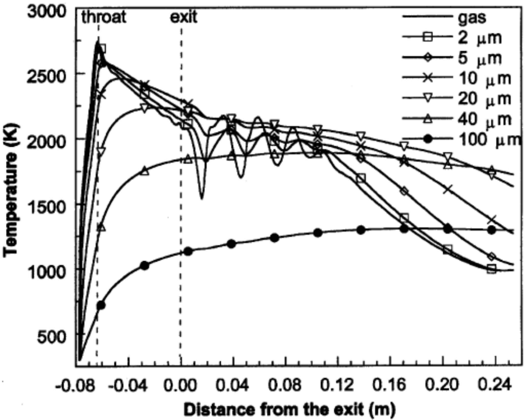
Cheng et al. [82] applied Ganser’s drag coefficient correlation [83], which is a function of particle sphericity index, to model the drag force acting on the spherical and non-spherical particles. Figure 9 illustrates the axial velocities of the gas flow and the spherical particles with different diameters during flight [82]. As it is shown in Figure 9, the gas flow velocity fluctuates in the shock diamonds section and drops after this part. The particle velocity strongly depends on the particle size. As the particle size reduces, the magnitude of acceleration and deceleration of the particle increases. The predicted temperatures of the gas flow and spherical particles with different diameters at the centerline of the nozzle are shown in Figure 10. The smaller particles are heated up and cooled down more rapidly and very fine particles follow the gas temperature behavior. It was suggested that for very fine particles (i.e., nanostructured coatings), it is better to decrease the spray distance. Authors also studied the in-flight behavior of non-spherical particles. The oblate spheroidal particles with the same volume diameter but different aspect ratio, E, were considered. The aspect ratio was defined as the ratio of shortest length to longest length of an elliptical shape (E = 1 for spherical particle). As the aspect ratio or equivalent sphericity decreased, the particle velocity increased and the particle was heated up and cooled down more rapidly (especially for E < 0.5).
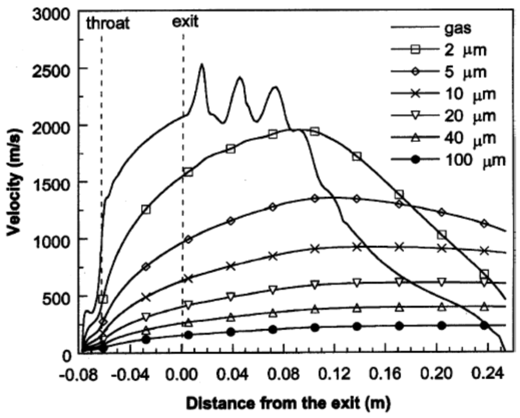
Figure 9.
Predicted axial velocities (at the jet centerline) of the gas phase and spherical particles with various diameters during flight. Reprinted with permission from [82] (Copyright 2001 by The Minerals, Metals & Materials Society and ASM International).
Figure 9.
Predicted axial velocities (at the jet centerline) of the gas phase and spherical particles with various diameters during flight. Reprinted with permission from [82] (Copyright 2001 by The Minerals, Metals & Materials Society and ASM International).


Figure 10.
Predicted temperatures (at the jet centerline) of the gas phase and spherical particles with various diameters during flight. Reprinted with permission from [82] (Copyright 2001 by The Minerals, Metals & Materials Society and ASM International).
Figure 10.
Predicted temperatures (at the jet centerline) of the gas phase and spherical particles with various diameters during flight. Reprinted with permission from [82] (Copyright 2001 by The Minerals, Metals & Materials Society and ASM International).
Kamnis and Gu [84,85] simulated the in-flight behavior of non-spherical WC-Co powder injected into a liquid-fueled (kerosene) HVOF torch. Fuel and oxygen were axially injected into the combustion chamber and particles were radially injected into the barrel. The drag coefficient was assumed to be a function of sphericity degree. They showed that, in comparison with spherical particles, non-spherical particles had higher axial velocities, lower temperature, and stayed closer to the torch centerline. However, as the particle size decreased, the effect of the aspect ratio (sphericity degree) on the particle behavior became less important.
3.4. Powder Injector Effects
Hackett and Settles [86] examined the effect of powder injector location on particle velocity and temperature. Powder was injected from three different locations inside the combustion chamber and the nozzle throat. It was shown that the injector location did not have considerable effect on particle velocity in contrast to its significant influence on particle temperature. Li and Christofides [87] and Lopez et al. [88] also changed the particle injection position and found the same results. However, the injection position effect on the particle temperature became negligible when the particle size was small [87].
Gu et al. [9] showed that as the particle injection velocity (axial injection into the combustion chamber) increased, the particle temperature inside and outside the gun reduced slightly. However, the particle velocity inside and outside the gun was not affected by the increase in the particle injection velocity (similar results in [60,72,73]). In addition, the particle injector position was changed vertically and the particle trajectory, temperature, and velocity were analyzed. When the particle injector was not located at the centerline, the particles spread before the nozzle entrance and then converged towards the centerline. However, authors found that the spreading distance was small in comparison to the central port radius; therefore, all the particles were approximately collinear with the gun centerline during flight. The particle temperature increased and the particle velocity was not influenced as the particle injection distance from the axis increased.
Kamnis et al. [89] simulated the in-flight behavior of Inconel 718 particles injected into a liquid-fueled (kerosene) HVOF torch. Fuel and oxygen were axially injected through the central port into the combustion chamber and spherical particles were radially injected into the barrel through two holes with a tapping angle. Authors showed that for a specific range of particle injection speeds, the particle could travel across the gas flow and move towards the center of the jet. The particles that moved near the torch centerline gained more momentum and were heated more efficiently. Outside this specific range of injection speeds, particles either crossed the torch centerline and spread outwards or could not reach the torch centerline. In addition to the injection speed, particle diameter had significant influence on particle penetration into the gas flow. Small particles were blown away by the gas flow and spread outwards at the external domain (outside the nozzle). The injector location inside the barrel was changed and it was found that as the distance between the injector and nozzle throat decreased, higher particle temperature and impact velocity could be achieved (see [90] for similar results).
3.5. Nozzle Shape
Katanoda et al. [91,92] showed that as the nozzle surface roughness (friction) increases, the particle/gas velocity decreases and the particle/gas temperature increases in the downstream direction. As the cooling rate increases, the particle/gas velocity increases and the particle/gas temperature decreases in the downstream direction. Furthermore, when the axial length of the nozzle diverging part Ld was almost equal to the barrel length Lb, the highest particle velocity at the barrel exit was obtained. By assuming Lb/Ld = 1, the length Ld + Lb was changed and it was found that as this length increases, the particle velocity and temperature at the barrel exit increase [92].
Kadyrov et al. [70] revealed that the particle velocity in the supersonic nozzle was higher than that in the subsonic nozzle. However, the particle temperature in the supersonic nozzle was lower because the particle spent a shorter time in this nozzle. Yang and Eidelman [75] and Cheng et al. [71] showed that by increasing the barrel length, the particle velocity at the gun exit enhanced. The effect of the combustion chamber length on the particle phase behavior was analyzed by Gu et al. [9] and it was concluded that this length had a significant influence on the particle temperature and oxidation. As the combustion chamber length increased, the particle residence time in the high temperature region increased which caused more particle heating with minute change in velocity.
Hassan et al. [93] and Lopez et al. [88] studied the gas and particle phases’ behavior inside the “curved” aircap (the Metco diamond jet rotating wire torch). It was found that, at the aircap exit, the flow was not uniform since there were some regions where the flow was subsonic and was sucked from the ambient [93]. In addition, a wake area above the leeside of the wire tip and the boundary layer separation at the sharp corner of the torch were obtained. Therefore, the spray angle was found to be different from the geometric turn angle.
Dolatabadi et al. [63,64] attached a cylindrical shroud to the end of the HVOF nozzle (Sulzer Metco DJ2700 gun) and investigated the effects of the cylindrical shroud on the gas and particle phases both experimentally and numerically. To simulate the propylene and oxygen premixed combustion process, a multi-reaction (four-step reaction mechanism [8]) eddy dissipation model was used. Their study showed that using a shroud can significantly decrease the oxygen content in the coating due to reduction in penetration of the ambient air into the jet. The existence of less oxygen results in a reduction of particle oxidation. It is interesting to know that oxidation on the surface of metal particles happens due to the high oxygen concentration and high temperature around the particle [94]. It is generally believed that decreasing the oxygen content in the coating has positive influences on the mechanical properties, which improves the performance of coated products [63,64,95,96]. It was shown that using a shroud caused the coating porosity to increase slightly because it resulted in the decrease of the particle velocity (because of large re-circulating flow occurring at the beginning of the shroud) and the increase of particle temperature. Noting that, their model underestimated the particle temperature and velocity [63,64]. It was explained that ignoring the particle oxidation was the main reason of the discrepancy. Particle oxidation is an exothermic reaction and causes the particle temperature to increase.
The effect of the increase in length of the nozzle convergent part on the deposition efficiency, coating microstructure, and hardness was numerically and experimentally investigated by Sakaki and Shimizu [97]. The deposition efficiency is defined as [31]
According to reference [31], in a typical HVOF process, DE is around 50%. Sakaki and Shimizu [97] showed that as the convergent part length increased, the degree of particle melting increased; however, the particle velocity decreased slightly. In addition, the deposition efficiency and cross-sectional hardness of Al2O3-40 mass% TiO2 coatings grew as the convergent part length of the nozzle increased. Baik and Kim [98] and Kim and Kim [99] changed the nozzle throat diameter and the divergent section length to study the nozzle shape effect on the HVOF performance. As the nozzle throat diameter increased, the location of the Mach shock disc moved backward (it moved toward the nozzle) and the exhaust gas velocity reduced. In addition, as the divergent section length increased, the gas velocity and pressure beyond the nozzle throat increased and slightly decreased, respectively [98].
3.6. Shock Diamonds
Kamnis and Gu [66] used different types of numerical methods to simulate the HVOF system. The first order upwind and the third order QUICK (quadratic upstream interpolation for convective kinematics) schemes were used and it was shown that the upwind scheme could only predict two shock diamonds while the QUICK scheme was able to capture six shock diamonds. Interestingly, a series of shock diamonds was observed inside the nozzle and vanished in the barrel (similar results in [61,62]).
Dolatabadi et al. [31] used an Eulerian-Eulerian approach based on the compressible non-reactive gas/solid particle flow assumption to study the solid particles’ interaction with shocks and expansion fans. As mentioned earlier, this approach is suitable for the dense suspension of solid particles. In a HVOF system, in the area around the nozzle centerline, the local particle loading is relatively high and the suspension can be considered dense. It was shown that the particle number density was high near the centerline and the suspension became dilute in the zones far from the centerline. In comparison with the single-phase flow, the shock diamonds in two-phase flow shifted to the dilute area away from the centerline, meaning that the gas flow (in the two-phase flow case) in the region near the centerline, where most of the particles move, becomes subsonic. The gas velocity reduction leads to a decrease of the particle velocity. As the particle velocity reduces, the deposition efficiency decreases because the velocities of many particles are smaller than the minimum velocity required for the particle to be coated. They concluded that the position and strength of the shock diamonds depended on the amount of the particle loading, and if the particle loading was high enough, all the shock diamonds died away. Moreover, they illustrated that the trajectory deviation occurred for the particles moving off the centerline, and it magnified for particles moving away from the centerline [31,32].
Dolatabadi et al. [100] indicated that the particle trajectory deviation mostly happened inside the shock diamonds (using a DJ2700 gun). They also revealed that the small particles were repeatedly accelerated and decelerated while passing through the shock diamonds. Furthermore, they captured the spatial and velocity distribution of spherical and non-spherical particles at a standoff distance of 100 mm. They showed that due to the influence of shock diamonds and Mach disks, there was a smaller number of particles close to the centerline and a bimodal spatial distribution of the particles was observed. However, the particles that moved near the centerline had the maximum velocity. It is clear that the particle trajectory deviation from the centerline can negatively affect the coating quality. The spatial distribution of the non-spherical particles was even more unfavorable.
Dolatabadi et al. [100] also designed two nozzle attachments (diverging (D) and diverging-converging (D-C)) to improve the deposition efficiency, and to reduce the in-flight particle oxidation. Their goal was to eliminate the shock diamonds so that the supersonic flow could transit to the subsonic flow smoothly. They showed that with the D-C attachment, the supersonic flow was extended further outside the nozzle, the shock diamonds were diminished, and the supersonic to subsonic transition was much smoother. Therefore, the D-C attachment caused less particle deviation and more efficient particle acceleration (the particle velocity increased with the D-C attachment) than those without the attachment case. The residence time of the particle at the high temperature region decreased as the particle speed increased. Therefore, the D-C attachment provided a higher gas temperature but a lower particle temperature. It also caused the oxide formation in the coating to decrease due to the mixing rate reduction of the ambient air and the main stream.
3.7. Particle Oxidation Modeling
Zeoli et al. [94] added an oxidation model to the Lagrangian formula of particle tracking to study the oxide layer growth on in-flight metal (stainless steel) particles. The oxidation model was based on the Mott-Cabrera theory [101] for thin oxide films (the main assumption was constraint of oxidation by the ion transport through the oxide layer). Kerosene and oxygen were axially injected through the central port into the combustion chamber. The drag coefficient for non-spherical particles given by Haider and Levenspiel [102] was used. The particle temperature was computed by the exact solution of the heat conduction equation inside the particle. In this paper, particles with various diameters were released at different locations inside the nozzle. Authors showed that the oxide layer growth on the particle was strongly dependent on the particle diameter. As the particle size reduced, the oxide layer thickness increased. It should be noted that the particle surface-area-to-volume ratio increases as the particle size decreases. Therefore, a smaller particle heats up and reacts with oxygen more rapidly. In addition, it was shown that when the particle temperature was low, the oxidation progressed slowly. Authors mentioned that the fastest oxidation occurred when both oxygen concentration and temperature were close to their maximum values. They also compared the oxide layer growth on the particles released at convergent and divergent parts of the nozzle. It was displayed that oxide layer thickness on the particles released at the nozzle convergent part was higher.
3.8. Substrate Effects
The spray (standoff) distance has a significant effect on both particle velocity and temperature, particularly when the particle size is less than 30 µm [60,69,103]. In the work of Li and Christofides [60], as the spray distance increased from 20 to 30 cm, the small particles’ velocity and temperature decreased at the point of impact on the substrate. Li and Christofides [87] showed that many particles were not deposited on the substrate in a perpendicular way due to high radial gas velocity near the substrate (stagnation flow effects). In fact, small particles may fully track the gas stream and not adhere to the substrate [69,87,103]. Relatively small particles might be deposited on the substrate, but both the impinging velocity and angle are smaller than the ones of large particles. Ait-Messaoudene and El-hadj [81] concluded that the substrate presence causes the particle velocity and temperature to drop.
Srivatsan and Dolatabadi [65] modeled the effect of substrate geometry (flat plate, convex, and concave) on the main flow field and the particle velocity, temperature, and trajectory. The standoff distance was 25 cm and the DJ2700 gun was modeled. Interestingly, a bow shock was observed near the substrate. As a result, the particle impact velocity and the particle chance to land on the substrate decreased. Evidently, the bow shock location and strength depend on the substrate shape and standoff distance. Authors explained that smaller particles were more affected by the shock diamonds and the bow shock. In comparison with convex substrate, the strength of bow shocks formed on the concave and flat surfaces was high which caused most of the fine particles to deviate.
In summary, it can be concluded that, depositing nano and submicron particles on the substrate using typical HVOF torches is very difficult. Therefore, to generate nanostructured coatings, a new approach is required. In the next section, the high velocity suspension flame spray (HVSFS) technique, which is a proper approach to achieve this goal, will be discussed. In addition, even though there are several papers and studies related to gas-fueled HVOF systems, the liquid-fueled HVOF torches are still needed to be investigated. Modeling the liquid-fueled HVOF systems is complex due to the presence of various phenomena such as fuel droplet break up and combustion. As discussed above, there are some preliminary works related to the modeling of liquid-fueled HVOF torches; however, more accurate models are needed to estimate the droplet/particle temperature, velocity, and trajectory, and to optimize the torch. The next section is associated with understanding the phenomena involved in the liquid-fueled HVOF processes and provides descriptions of the numerous methods to simulate them.
4. High Velocity Suspension Flame Spray (HVSFS) Technique
As fine microstructured coatings have great performance, coatings with nano- and submicron-sized particles are the main trend in the development of emerging thermal spray processes. There are various unique properties related to fine microstructured coatings such as enhanced catalytic behavior, noticeable superhydrophobicity [104,105,106,107,108,109,110,111] behavior, remarkable wear resistance, superior thermal insulation and thermal shock resistance [7,112,113,114]. Nevertheless, coating fine particles using conventional atmospheric thermal spray techniques is a difficult task to do due to several reasons. The first reason is that particles usually form agglomerates which lead to clogging the feed lines, which makes it difficult to feed nano and submicron particles into the gas flow. The second reason is the strong tracking of gas phase streamlines by the submicron particles. In other words, very fine particles decelerate and get diverted by the gas flow in the stagnation region near the substrate. The third reason is the easy distribution of nano-scaled particles in air, which leads to their penetration in human skin or passing through the respiratory tract, the lungs, and finally entering the blood circuit.
To address the above-mentioned issues, spraying a suspension of fine solid particles is one of the best known techniques [7,115]. A combination of fine solid particles (usually in the range 500 nm–5 µm) and a base fluid such as water or alcohol is known as a suspension. To stabilize the suspension (preventing particle agglomeration and sedimentation) proper chemical stabilizers or surfactants are usually added to the system [115]. Suspension is commonly performed with the APS and HVOF techniques that are named as suspension plasma spraying (SPS) and high velocity suspension flame spraying (HVSFS). Instead of powder injection, a suspension is injected into the jet or flame using spray atomization or the injection of continuous jet methods (see Figure 11) [116]. In the HVSFS process, the suspension is usually injected into the combustion chamber directly. In this technique, the suspension has to be delivered against the combustion chamber pressure. Two different suspension feeder systems are designed and tested for this purpose: mechanical pumping of the suspension using a piston pump, and suspension transport through a pressure vessel that is operated with compressed gas [117]. In addition, the suspension can be injected into the divergent part of the HVOF nozzle radially. The external radial injection of suspension into the high temperature jet is used as well [116].
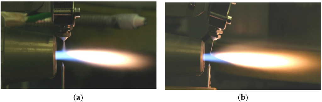
Figure 11.
External radial injection of suspension into HVOF jet: (a) Spray atomization and (b) Mechanical injection (continuous jet). Reprinted with permission from [116] (Copyright Elsevier 2009).
Figure 11.
External radial injection of suspension into HVOF jet: (a) Spray atomization and (b) Mechanical injection (continuous jet). Reprinted with permission from [116] (Copyright Elsevier 2009).

Figure 12 shows a schematic of the suspension droplet evolution in a high temperature jet or flame [115]. After suspension injection, the flame/jet atomizes the suspension (primary and secondary breakup) firstly, and the liquid evaporation becomes dominant subsequently. Because of liquid evaporation, the solid particles or their agglomerations remain in the field and the flame/jet temperature decreases. Then, the particles are heated up by the flame/jet and accelerated toward the substrate. It should be noted that the strong cooling of the hot gases by liquid vaporization and the very low inertia of particles implies very short spray distances [115,118,119].
Figure 12.
A schematic of a suspension droplet evolution in a high temperature jet or flame. Reprinted with permission from [115] (Copyright Elsevier 2009).
Figure 12.
A schematic of a suspension droplet evolution in a high temperature jet or flame. Reprinted with permission from [115] (Copyright Elsevier 2009).

It is clear that the coating quality obtained by the suspension spraying technique depends on the suspension penetration within the jet, the primary and secondary atomization of the suspension, and the slurry droplet evaporation/combustion [115,118]. To control the above-mentioned phenomena, the suspension characteristics such as density, specific heat, viscosity, surface tension, thermal conductivity and velocity as well as the main flow properties, momentum, temperature, pressure, and turbulence should be known. It should be noted that the mentioned suspension properties strongly depend on the particle concentration, particle material, size and shape, base fluid material, surfactant/additives composition and concentration, suspension temperature, and acidity (pH) [120,121,122,123,124]. The significance of most of the mentioned parameters related to the coating properties has not been explored yet. Moreover, the type of suspension injector is important. It can be very simple, such as cylindrical and conical injectors, or very complex, such as twin-fluid injectors (e.g., effervescent). In addition, the location and angle of the injector have some influences on the coating properties and should be studied [50,116,120].
4.1. Suspension Properties
Thermal conductivity, viscosity, specific heat, surface tension, and density of suspension have significant influences on the suspension breakup and evaporation/combustion. In addition, suspension properties are the input values for the numerical solver and should be known. It should be noted that understanding and predicting the properties of suspensions is an active research area [121,122]. Most suspension properties are obtained from the experiments and there is no comprehensive theory to cover all effective parameters such as temperature, particle concentration, particle material, and particle size [121,122]. Although there are some empirical and theoretical equations for predicting the suspension and nanofluid properties, all the proposed equations have serious limitations. These equations are mainly proposed for a specific particle size, material, and volume concentration [122]. In addition, most of studies are focused on the materials which are typically utilized for cooling systems or propulsion [121,122,123,124,125,126,127,128]. In coating technology, most suspension properties are still unknowns. In this paper, the most famous empirical and theoretical equations for predicting suspension properties are presented.
The density of suspension ρ is given by
where αp, ρp and ρl are the particle volume fraction, the particle density, and liquid density, respectively [22,122]. The following correlation, which is very similar to the density equation, has been widely used to calculate the specific heat C of suspensions
where Cp and Cl are the particle-specific heat and the liquid-specific heat, respectively [122].
In general, the thermal conductivity of a suspension is higher than that of a base fluid. For a dilute suspension (particle volume fraction less than 1%) of relatively large particles (submicron and micron-sized particles) in fluids, the Maxwell equation is usually used to describe the thermal conductivity of suspension (k) as a function of particle phase volume fraction αp [121,126]
where kp and kl are the thermal conductivity of the particle and liquid phases, respectively. The Bruggeman equation is also used to predict the thermal conductivity of suspension and is as follows [123]
However, for nanofluids where the particle size is usually less than 100 nm, the above equations are not able to predict satisfactory results. In general, all equations proposed by researchers for the thermal conductivity of nanofluids have serious limitations [121,122].
Generally, the viscosity of suspensions and nanofluids is greater than that of base fluid. It is clear that the viscosity of suspension and nanofluid strongly depends on particle volume fraction. For instance, when the base fluid is Newtonian, a dilute suspension usually exhibits a Newtonian behavior, and suspensions at low to moderate solid concentrations are usually pseudoplastic (this is also termed shear-thinning). It is also not unusual for suspensions that are pseudoplastic at low to moderate solid concentrations to become dilatant (shear-thickening) at high solid concentrations [123]. The following correlations are proposed to describe the suspension viscosity (μ) in terms of the base fluid viscosity μ0 and particle volume fraction αp [123,124]:
Einstein’s equation
Simha equation for anisometric particles
where a is the major particle dimension and b the minor particle dimension.
Einstein-Batchelor’s equation
Thomas’s equation
Einstein’s model is the first equation proposed for suspension viscosity. Other mentioned equations are extending the validity of Einstein’s formula. These equations apply to Newtonian behavior and usually require that the particles not be too large (applicable for submicron and micron-sized particles) and have no strong electrostatic interactions (applicable for dilute suspensions (αp ≈ 1%) with non-interacting spherical solids).
The more often-applied, semiempirical models in suspension are as follows (Baker-type equations)
in which a common analogue is the Krieger-Dougherty equation [124,127]
where is the maximum packing volume fraction [127]. By the appropriate choice of , the effect of particle shape, size, size distribution, and even porosity can all be taken into account. At high particle loadings, the Einstein-type equations perform expectedly poor, although their parameters are more straightforward than those of Baker. In general, among the above equations, the Krieger-Dougherty equation can predict suitable results for dilute and dense flows [124,127]. Similar to the thermal conductivity case, all equations proposed by researchers for the viscosity of nanofluids have serious limitations [122].
The only useful resources to estimate the suspension surface tension are a few experimental data in the literature. The equilibrium (static) surface tension strongly depends on the particle size, material (particle wettability), volume fraction, base fluid material, surfactant, and temperature [125]. In general, the equilibrium surface tension of a fluid is reduced from its pure-fluid value when materials such as surfactants adsorb at the interface [125,128,129]. In addition, even in the experimental results, it is not yet clear that adding very fine particles to a liquid causes the surface tension to decrease or increase [125,128,129,130]. For example, adding hydrophobic (non-wetting) particles to a fluid usually causes the surface tension to decrease because hydrophobic particles are able to attach to the gas-liquid interface (particle adsorption at the interface) [130,131,132]. On the other hand, when hydrophilic (water-wet) particles such as metal oxides are added to a fluid, the surface tension slightly increases or decreases from its pure fluid value because the hydrophilic particles do not collect, or adsorb, at the gas-liquid interface. In other words, hydrophilic particles do not reduce the equilibrium surface tension significantly because they generally do not collect, or adsorb, at the interface [128,130].
As mentioned above, the presence of surfactant in suspensions can change the surface tension significantly. A surfactant molecule consists of two parts: a hydrophilic part and a hydrophobic part [133,134]. Therefore, there is always one part of the molecule that does not like the solvent environment. As a result, the surfactant molecules migrate to surfaces and interfaces, and change the interfacial surface tension. As the surfactant concentration increases, the equilibrium (static) surface tension (it can be measured by du Nouy ring method [135]) reduces and is minimized at a certain concentration of surfactant called the critical micelle concentration (CMC) [136]. The static surface tension remains relatively constant for surfactant concentrations greater than the CMC. It is also clear that the surfactant molecules need a certain time to reach the surface/interface. This time can change from milliseconds to days depending upon the composition and concentration of surfactants. Despite the fact that the surface tension is a function of time, it is called dynamic surface tension. Since the surface tension value has significant influence on the spray properties and droplet sizes, the accurate value should be used to model the breakup phenomenon. It is proved that the dynamic surface tension is more appropriate than the static surface tension to study the spray characteristics of surfactant solutions and suspensions [136]. Measurements of oscillating free jets, where a fluid comes out of an elliptical nozzle, together with an analytical model have long been used to determine the dynamic surface tension [137,138,139,140,141,142,143,144,145]. Noticeably, the value of the surface tension of pure fluid can only be applied for a dilute suspension with a low concentration of surfactant.
4.2. Breakup
It is known that the interaction between the gas and the liquid flow results in a rapid fragmentation of the liquid into a flow of droplets. Noting that, during the liquid breakup process the surface-to-volume ratio in liquid is increased [146,147]. The breakup process contains three main steps: liquid flow ejection, the primary breakup, and the secondary breakup mechanisms. Once the liquid flow initiates from the nozzle, deformations start to appear on the liquid interface. The deformations grow in time and space, which ultimately lead to liquid fragment ejection from the main liquid flow. The primary breakup mechanism is created from the initial flow deformation and the subsequent liquid fragments formation. The liquid fragments might distort and breakdown into smaller elements which constitute the secondary breakup mechanism. When surface tension forces are strong enough to ensure the liquid fragment cohesion, the stable drops are formed. In the following sections, the details of the mentioned steps will be discussed.
4.2.1. Primary Breakup
Cylindrical Liquid Jet Breakup
To understand the mechanism of primary breakup in detail, the behavior of cylindrical liquid jets discharging into a quiescent gaseous that are widely used in suspension thermal spray processes will be discussed first. Forcing the liquid to pass through a cylindrical tube of length L and diameter D results in the formation of cylindrical jets. Five regimes known as dripping, Rayleigh, first wind-induced, second wind-induced, and atomization are involved in the analysis of cylindrical jets (Figure 13). In the dripping regime, drops are directly discharged from the nozzle exit without continuous liquid column formation. By increasing the liquid jet speed, the continuous liquid column is formed and the capillary forces become dominant in the process. This regime is named the Rayleigh breakup regime. In both mentioned regimes, droplet pinching occurs axisymmetrically, which leads to the formation of drops with a comparable size to the orifice diameter. In the Rayleigh regime, an axisymmetric perturbation that has a wavelength of the same order of magnitude as the jet diameter disturbs the liquid column (Figure 13). Drops get detached from the jet when the perturbation amplitude becomes equal to the jet radius. Higher jet speeds result in aerodynamic interactions with the ambient gas, which creates additional surface instability (i.e., wind-induced regime). As can be seen from Figure 13, a dominant perturbation evolving on the liquid jet interface is still observable in the first wind-induced regime. Noting that, the drop production in this regime is not as organized as in the Rayleigh regime, although the perturbation is still rather axisymmetric. In the second wind-induced regime, the jet column is perturbed at the nozzle exit and becomes chaotic as the perturbations grow. There are two main breakup mechanisms in the second wind-induced regime. The first one occurs near the nozzle exit, where small droplets are peeled off the liquid jet interface. Farther downstream, the second primary breakup mechanism can be noticed where the remaining liquid flow disintegrates into large liquid fragments. At higher jet velocities, the atomization regime occurs that is characterized by the spray appearance. A series of small drops around a liquid core that get vanished eventually downstream of the orifice are observable (Figure 13). The intact core length may either decrease or increase (depending on fluid properties and orifice design) with a further increase in jet speed within the atomization region. Noting that, the average drop size is much less than the jet diameter in this regime [146,147,148,149].

Figure 13.
Cylindrical jet behavior and breakup regimes; (top) stability curve; (bottom) visualization examples; from left to right: Rayleigh regime (B) ReL = 790, WeG = 0.06; first wind-induced regime (C) ReL = 5500, WeG = 2.7; second wind-induced regime (D) ReL = 16500, WeG = 24; atomization regime (E) ReL = 28000, WeG = 70. Reproduced from Reference [146] with permission (Copyright Springer 2008).
The liquid-gas interfacial forces and the internal flow structure (turbulence and cavitation) are the most effective parameters on liquid jet behavior in the second wind-induced and atomization regimes. The mixing rates are augmented with the liquid jet turbulence level at the nozzle orifice [146,150]. Liquid cavitation that might occur at the injector orifice influences the jets’ behavior in the second wind-induced and atomization regimes as well. The local pressure downstream of the orifice inlet corner may be low enough to form flow local cavitation, depending on the liquid velocity, overall pressure drop, and orifice inlet shape [146]. Figure 14 schematically shows the cylindrical jet appearance as a function of cavitation. It is revealed that the orifice shape is the main parameter in initializing the cavitation. It is known that conical or round-inlet discharge nozzle prevents cavitation growth in the discharge orifice, in contrast to sharp-edged inlet nozzles that promote cavitation.

Figure 14.
Cylindrical jet schematic appearance as a function of cavitation [146,151].
Figure 14.
Cylindrical jet schematic appearance as a function of cavitation [146,151].
The effect of the nozzle aspect ratio (L/D), which mainly controls the liquid velocity profile at the nozzle exit, on the breakup length of the liquid jet is illustrated in Figure 15 [151,152,153].

Figure 15.
Nozzle aspect ratio effects (A.R. = L/D) on the breakup length of cylindrical jets [152].
Figure 15.
Nozzle aspect ratio effects (A.R. = L/D) on the breakup length of cylindrical jets [152].
In general, increasing the nozzle’s aspect ratio results in a shorter breakup length. As the nozzle length increases, the liquid jet turbulence level at the nozzle exit enhances, which causes the breakup length to decrease. However, for very large aspect ratios such as L/D = 50, the flow inside the nozzle becomes fully developed which results in the increase of breakup length. Moreover, cavitation taking place inside the nozzle can change the mentioned consistency. It is also proven that the aspect ratio effects are severe at standard atmospheric pressure, unlike at high ambient pressure [151,152,153].
The ambient properties’ effect, particularly the ambient gas density, is significant in the atomization regime. The liquid jet might fragment into droplets with diameters much smaller than the jet diameter if the gas inertia force (which is proportional to the gas density) is large enough [154]. In other words, at elevated ambient pressures (i.e., density), aerodynamic effects become very important and a fine spray might be produced by the liquid jet [155]. Increasing the ambient pressure (i.e., density) decreases the jet breakup length and results in a larger spray angle in addition to production of rougher jet surfaces [151,152,153,156,157,158,159,160]. Reitz and Bracco [160] noted that when low-speed fluid is injected into a highly pressurized (high density) environment, the atomization regime can be gained. In addition, they revealed that the intact column length decreases with increasing ambient pressure.
Table 1 shows the criteria for evaluating the nature of cylindrical liquid jet breakup. The values of the gaseous Weber number, WeG, liquid Weber number, WeL, and Ohnesorge number, Oh, should be calculated to evaluate the Rayleigh and first-induced regimes. However, the gaseous Weber number, the liquid-to-gas density ratio, and the Taylor parameter, T, are involved in the second wind-induced and atomization regimes. These numbers are as follows
where μL is the liquid dynamic viscosity, UL is the liquid average velocity, σ is the surface tension coefficient, D is the nozzle diameter, and ρL and ρG are the liquid and gas densities, respectively [146].

Table 1.
Criteria used in evaluating the regimes of cylindrical liquid jet breakup [146,161,162,163,164,165].
| Breakup Regime | Criteria |
|---|---|
| Region A: dripping regime | WeL < 8 |
| Region B: Rayleigh regime | WeL > 8 WeG < 0.4 or 1.2 + 3.41Oh0.9 |
| Region C: first wind-induced regime | 1.2 + 3.41Oh0.9 < WeG < 13 |
| Region D: second wind-induced regime | 13 < WeG < 40.3 |
| Region E: atomization regime | 40.3 < WeG |
Another admired way to categorize the cylindrical jet breakup is Ohnesorge’s classification. In this method, the breakup regimes are shown on a logarithmic plot of the Reynolds number, Re, versus the Ohnesorge number, Oh, which is revealed in Figure 16 [148,166,167]. Overall, the liquid jet breakup is delayed by increasing the fluid viscosity as the internal fluid turbulence and instabilities are strongly dampened. However, for high Weber and Reynolds numbers the liquid viscosity does not affect the primary breakup, unlike the secondary breakup that is influenced.

Figure 16.
Ohnesorge’s classification for categorizing the cylindrical liquid jet breakup, (a) Rayleigh regime; (b) first wind-induced regime; (c) second wind-induced regime; (d) atomization regime. Reproduced from Reference [166] with permission (Copyright Springer 2003).
Figure 16.
Ohnesorge’s classification for categorizing the cylindrical liquid jet breakup, (a) Rayleigh regime; (b) first wind-induced regime; (c) second wind-induced regime; (d) atomization regime. Reproduced from Reference [166] with permission (Copyright Springer 2003).
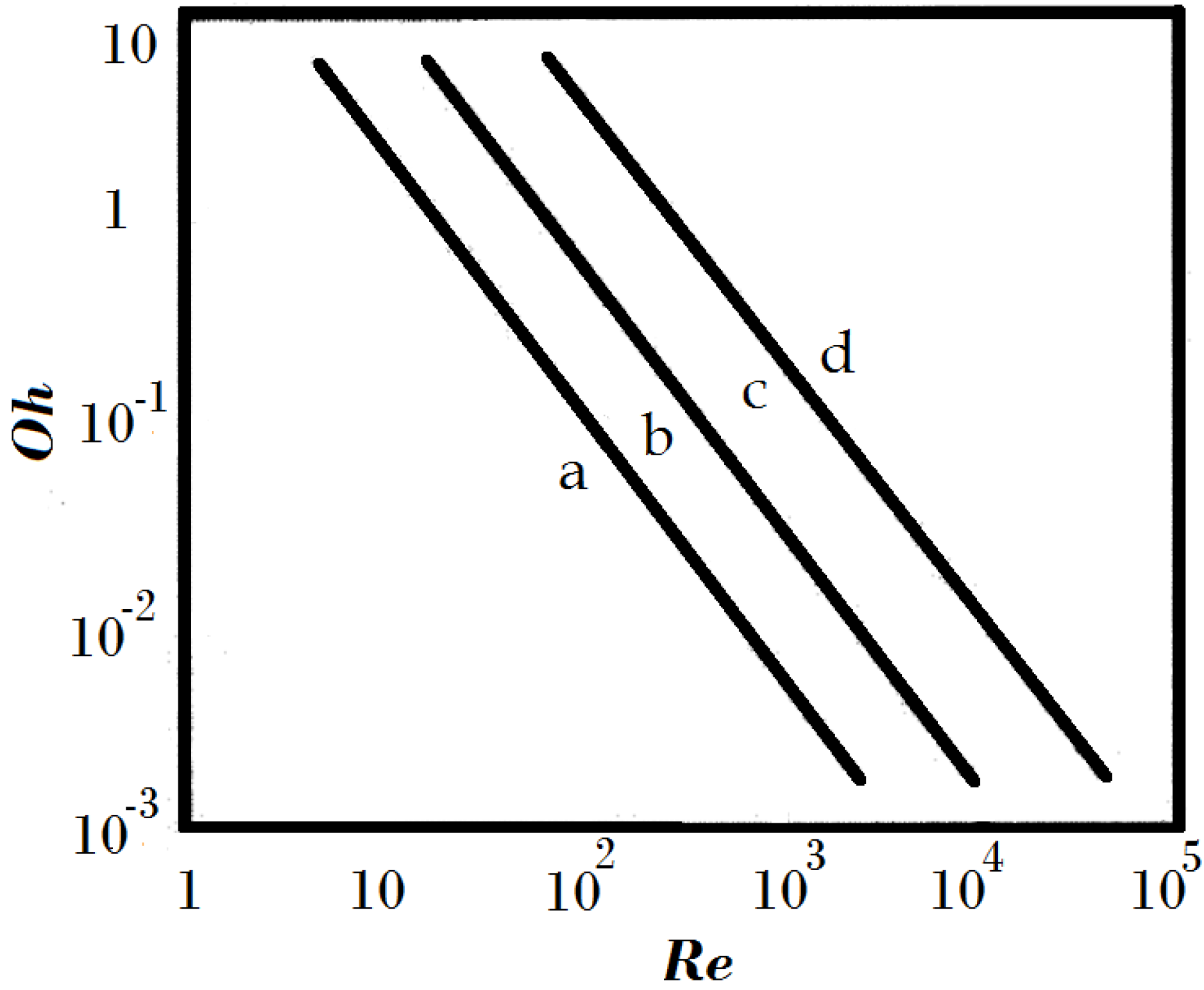
Liquid Jet in Crossflow
As mentioned above, in thermal spray processes, the liquid/suspension can be injected into the flame/jet radially. Therefore, an introduction and literature review into the subject of liquid jets breakup in a transverse gas flow (crossflow) is provided here (see Figure 17).
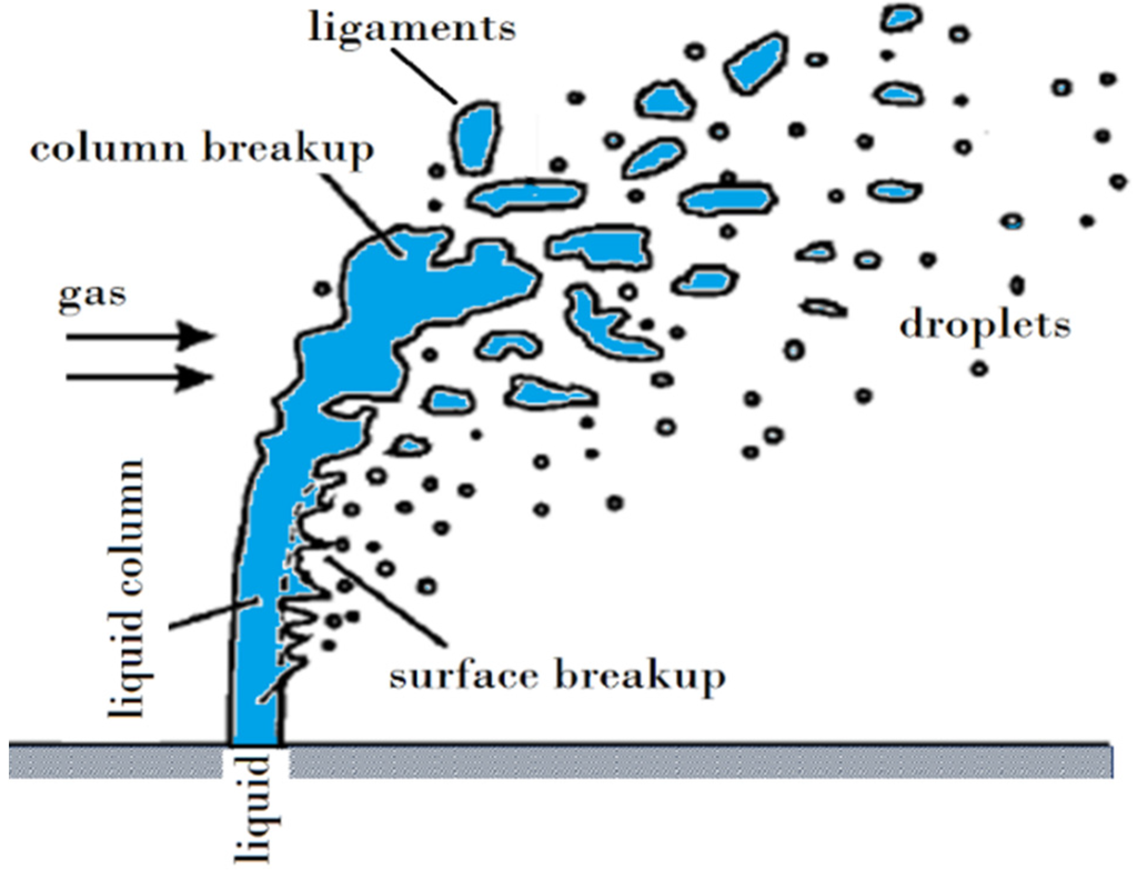
Figure 17.
Breakup of liquid jets in transverse subsonic airflow.
Figure 17.
Breakup of liquid jets in transverse subsonic airflow.

It is known that the liquid jet flattens and bends in the crossflow direction due to the presence of the crossflow dynamic pressure [168,169,170,171,172,173,174]. As it is demonstrated in Figure 17, the spray field generated by a jet in crossflow can be divided into three regions: (1) intact liquid column; (2) ligaments; and (3) droplets [173,174,175,176]. In the liquid column region, the instabilities are developed and lead to the formation of ligaments and droplets. The wave’s amplitude increases along the jet column (windward surface) until it breaks at one of the wave troughs [177,178]. Noting that, this rupture occurring at the wave trough, but not at every trough, results in the formation of short jet segments, named ligaments (referred to as the column breakup) [173,176]. The column breakup point (CBP) or the fracture point is referred to as the location where the liquid column stops to exist. The further breakup of ligaments into smaller droplets is referred to as the secondary breakup [176]. It should be noted that surface waves with short wavelength are also observed on the lower (leeward) surface of the liquid jet. Due to these waves’ interaction with the crossflow dynamic pressure, droplets are sheared off the leeward surface, which is known as surface breakup. In general, surface breakup results in the formation of droplets that are smaller than those produced from ligaments [173].
There are several effective parameters in the liquid jet crossflow phenomenon such as density, viscosity, and velocity of both phases, surface tension, duct width (L), and nozzle diameter (D) [179]. Based on the mentioned parameters, the following dimensionless groups are introduced
A breakup map in the plane of the momentum flux ratio q and the aerodynamic Weber number WeG was proposed by Wu et al. [173] to show different breakup regimes in crossflow (see Figure 18 and Figure 19). Noting that, the mentioned two parameters are the most relevant parameters in jet breakup criterion. At elevated pressure, similar breakup mechanisms and high correspondence with Wu et al.’s map [173] were found [177]. As can be seen from Figure 18, for low values of q and We, the column breakup is observed and the droplets are formed from ligaments. On the other hand, for high values of either q or We, surface breakup, which is the mechanism of droplet shearing-off from the jet walls, is observed. As both of these mechanisms might be active for a typical jet, the breakup mode will be determined by the dominant mechanism. However, as the Weber number increases, the surface breakup extent grows slowly, in a way that there will be a zone where both mentioned mechanisms are dominant. This zone is known as multimode breakup mode. Noting that, this mode is only a transition between the two modes that were defined earlier and is not a new mode [173,174,180].

Figure 18.
Regime map of liquid jets’ breakup processes in subsonic crossflow. Adapted from Reference [173] with permission (Copyright AIAA 1997).
Figure 18.
Regime map of liquid jets’ breakup processes in subsonic crossflow. Adapted from Reference [173] with permission (Copyright AIAA 1997).
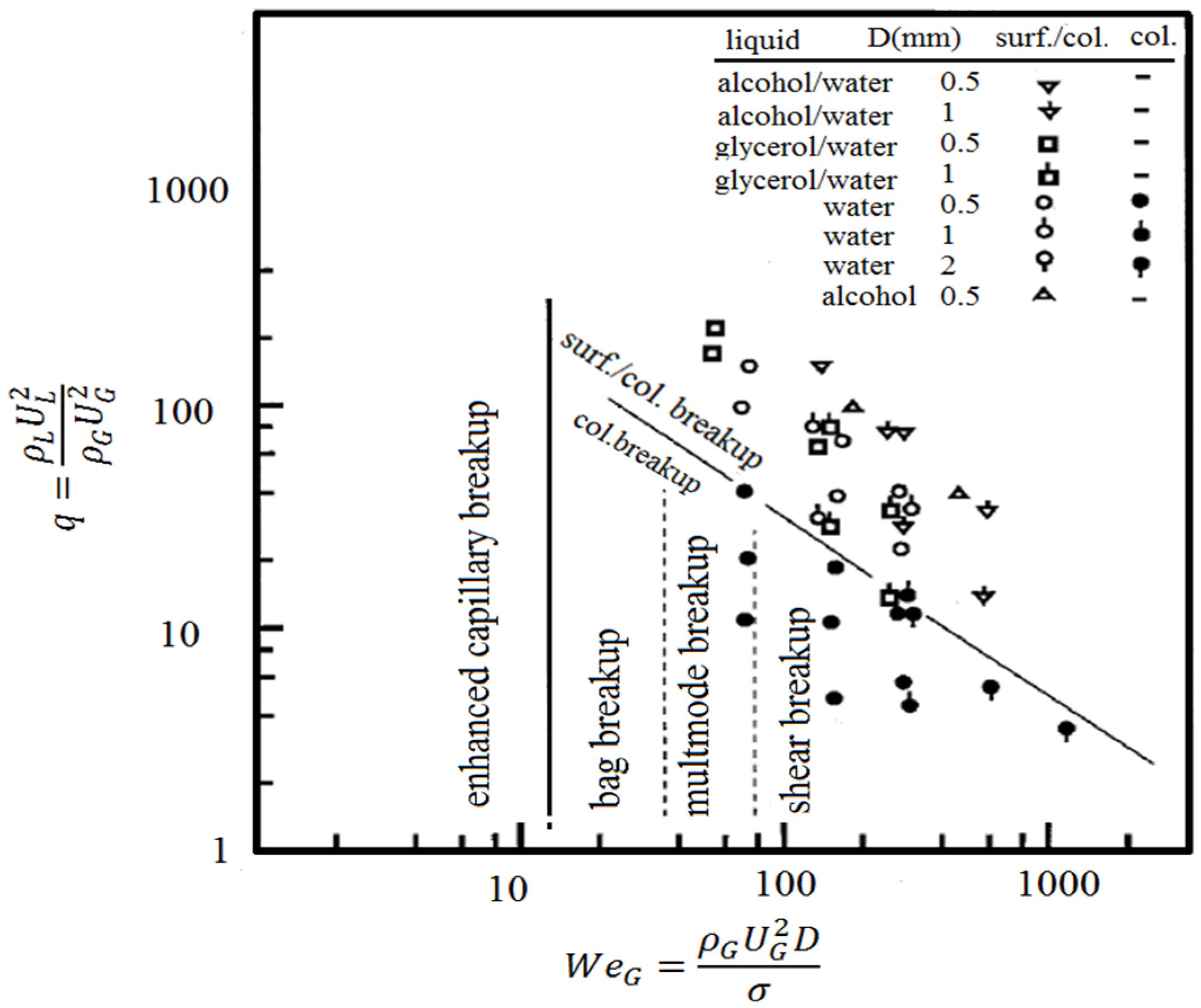
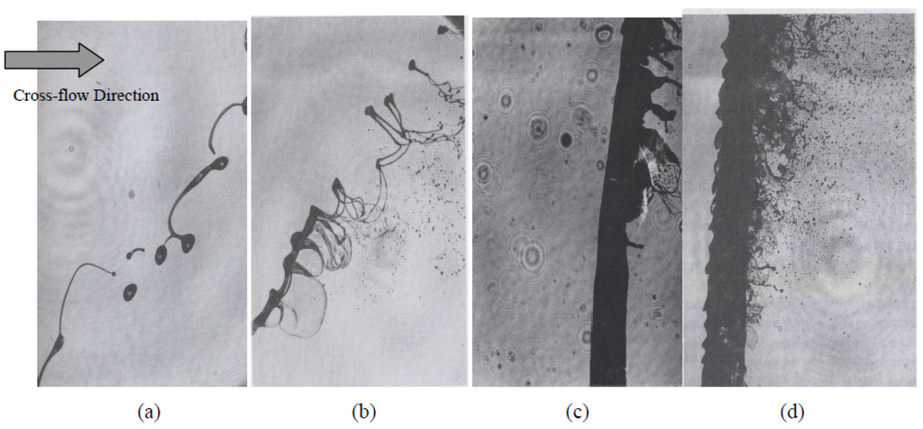
Figure 19.
Different types of liquid jet breakup in transverse subsonic gas flow: (a) Column breakup (enhanced capillary breakup); (b) bag breakup; (c) bag/shear (multimode) breakup; (d) shear breakup. Reproduced from Reference [181] with permission (Copyright AIP Publishing LLC 2012).
Figure 19.
Different types of liquid jet breakup in transverse subsonic gas flow: (a) Column breakup (enhanced capillary breakup); (b) bag breakup; (c) bag/shear (multimode) breakup; (d) shear breakup. Reproduced from Reference [181] with permission (Copyright AIP Publishing LLC 2012).
Two main parameters that characterize the liquid jet fragmentation in the crossflow are spray penetration into the crossflow and column breakup point (CBP) [176]. Various experiments are performed with different momentum flux ratios that lead to developing correlations between the dependence of the jets’ upper surface trajectory (windward) in a crossflow and the liquid-to-gas momentum flux ratio [173,174,175,176]. It was found that the surface breakup extent and the liquid penetration increase by increase of the q. Furthermore, increasing the We results in the decrease of the average droplet size; consequently, as smaller droplets decelerate faster, the overall spray penetration decreases. The size of the formed drops during fragmentation is dependent on the surface tension coefficient, σ, in a way that as lower surface tension has weaker resistance to breakup, smaller droplets will be formed [174]. Increasing the liquid viscosity reduces the penetration height due to increase of the drag force on the jet [182]. Additionally, compared to the smaller diameter jet, the liquid jet with a larger diameter penetrates further into the gas stream as it bends at a later streamwise distance [174]. It is observed that increasing the air stream temperature or the liquid jet temperature results in the decrease of the liquid jet penetration [183]. Furthermore, it is noticed that at a given q, an increase in the ambient pressure increases the breakup and decreases the liquid jet penetration [184,185].
Costa et al. [186] studied the problem of liquid injection into a crossflow gas stream from angled nozzles. They found that the jet angle plays a more important roll on spray characteristics than q. Lubarsky et al. [176] investigated the effect of injector internal design on the jet crossflow. Two injectors with the same orifice diameter and different internal path shape, sharp-edged and round-edged orifices, were used. Their study showed that due to creation of internal turbulence by the sharp edge at the orifice entrance, the liquid jet boundaries are changed which lead to the variations of the jet outer border structure and droplet size. In addition, they found that the liquid jet internal turbulence affects the CBP location [176]. Ahn et al. [187] showed that cavitation and hydraulic flip of the orifice internal flow result in considerable differences between the observed trajectories and the ones reported [173]. Nguyen and Karagozian [188] analytically studied the behavior of reacting liquid jets in subsonic crossflow. They described that in a low subsonic flow regime, it is likely to have a flame enveloping the cross-section. Any evaporation or other surface blowing decreases the momentum transmission from the gas to the liquid. However, they showed that the effect of evaporation on the jet trajectory shape is relatively insignificant.
Basically, all mentioned studies attempted to explain the liquid penetration trajectory into the crossflow using q, We, and certain functions that describe the shape of the spray outer edge. Although there are numerous available correlations in this matter, each of them proves different results, and their practical use remains problematic [176]. Some correlations for liquid jet trajectory and CBP location are as follows (the liquid jet and the crossflow are in the y and x directions, respectively):
Chen et al. [175]
Inamura et al. [189]
Becker et al. [177]
Masuda et al. [190]
Tambe et al. [174]
A correlation including the gas temperature effect was offered as below [183]
where T0 = 294 K. A correlation including the gas pressure effect was offered as below [184]
A correlation for maximum and average spray penetration including the injector internal shape effect was given as follows [176]
where the coefficients (a1 and a2) are presented in Table 2.
Table 2.
The values of coefficients (a1 and a2) used in Equation (52) for computing the average and maximum spray penetration into the crossflow [176].
| Injector Type | a1 | a2 | a1 | a2 |
|---|---|---|---|---|
| Sharp edge | 1.2181 | 1.8806 | 1.9866 | 0.7403 |
| Round edge | 1.0724 | 1.8641 | ||
| Penetration | Average | Maximum | ||
A popular correlation is prepared by Wu et al. [173]
Height of the column breakup point (CBP) [173]
Axial distance to the column breakup point (CBP) [173]
The above correlation indicates that there is a constant location where liquid jet breakup in the streamwise direction occurs. Some studies confirm this result though discrepancies in the numerical value of the location exist. However, Schetz and Padhye [191] and Lubarsky et al. [176] indicated that the streamwise location of CBP depends on q. Birouk et al. [192] showed that for very high viscosity liquids, the streamwise location of jet fracture is not only dependent on q, but also on the Ohnesorge number, Oh.
In the HVSFS process, a suspension/liquid can be injected into the divergent part of the nozzle radially. The interaction of the liquid jet with the supersonic crossflow produces a 3D bow shock [193] (see Figure 20). Consequently, the upstream wall boundary layer separates, creating a region where the boundary layer and the jet fluid mix subsonically upstream of the jet exit [194]. The surface waves exist in the near-injector region and with their growth, the liquid jet finally breaks up at the troughs [195].
As mentioned above, spray penetration is one of the key parameters that characterize the liquid jet breakup in the crossflow. Some penetration height correlations for transverse liquid jets in supersonic crossflow are given below:
Yates [193]
where Cd is the orifice discharge coefficient.
Ghenai et al. [194]
Lin et al. [196]
where θ (in deg.) is the injection angle relative to the freestream gas. Noting that, the liquid jet penetration height increases by increasing the momentum flux ratio q.

Figure 20.
Sketch of a typical liquid breakup process in the supersonic crossflow [193].
Figure 20.
Sketch of a typical liquid breakup process in the supersonic crossflow [193].
Coaxial Jets
The behavior of a cylindrical liquid jet surrounded by an annular gaseous stream (known as coaxial jets) will be discussed here. The liquid jet is injected through a cylindrical orifice (with the diameter DL) and the gas issues from a coaxial annular slit (with the internal outer diameter DG). The average velocities of liquid and gas phases are UL and UG, respectively. In addition to the dimensionless numbers introduced for the cylindrical liquid jet (Equation (43)), the relative gaseous Weber number WeR, the momentum flux ratio M, the gaseous Reynolds number ReG, the effective Reynolds number Reeff, the mass flux ratio m, and the area ratio A0 can also be defined as follows [146]
where AG and AL are the area of the gas and liquid flow outlets, respectively.
Farago and Chigier [197] classified the breakup regimes of the coaxial air-water jets into three categories: the Rayleigh-type breakup, the membrane-type breakup, and the fiber-type breakup (see Figure 21). When drops (with the diameter in order of the jet diameter) are generated without any liquid ligament or membrane shedding from the liquid flow, the breakup regime is Rayleigh-type. This regime can be divided in two subregimes, namely the axisymmetric subregime and the non-axisymmetric subregime. In the axisymmetric subregime (WeR < 15) the liquid jet is accelerated by the gas flow and demonstrates a shorter breakup length than in a still gaseous environment. The drops are formed from the growth of an axisymmetric wave. In the non-axisymmetric subregime (15 < WeR < 25), the liquid jet diameter is decreased by the gas flow and drops are still generated by the breakup of the flow as a whole. The membrane-type breakup (25 < WeR < 70) is obtained from the formation of thin liquid sheets, which create Kelvin-Helmholtz waves and disintegrate into droplets of much smaller diameter than the Rayleigh-type breakup regime. The fiber-type regime (100 < WeR < 500) is characterized by the formation of thin liquid fibers, which peel off the jet and breakup via the non-axisymmetric Rayleigh’s mechanism. The liquid core becomes wavy farther downstream, and disintegrates into ligaments from which new fibers are peeled off [146,197]. Farago and Chigier [197] divided the fiber-type regime in two sub-modes called pulsating and superpulsating. The normal mode of atomization is classified as the pulsating mode, whereas the superpulsating mode (150 < WeR < 500) is associated with an extremely high periodical change between high and low-density regions in the sprays [146,197]. They concluded that the superpulsating mode is dominant when ReL/ < 100. Mayer and Branam [198] found a criterion for the superpulsating mode identical to the mentioned correlation [197] but with an exponent for WeR equal to −0.4 instead of −0.5.
Lasheras et al. [199] observed the digitations-type breakup regime that was not described by Farago and Chigier [197]. This regime demonstrates the ligaments’ (digitations’) development on the crests of an axisymmetric perturbation and the subsequent disintegration of these ligaments by a non-axisymmetric Rayleigh’s mechanism [199,200,201]. They observed this regime for laminar liquid flow and turbulent gaseous flow [199]. Lasheras and Hopfinger [200] also reported that this regime lies in the membrane-type breakup regime of Farago and Chigier’s classification. In addition, Lasheras et al. [199] found that the fiber-type breakup regime is observable when WeR > 200 (this limit is greater than the limit reported by Farago and Chigier [197]). They also determined a critical value of M (order of 35) at which the liquid (water) cone is chopped off and the superpulsating mode is reached. Leroux et al. [202] observed the Rayleigh-type breakup regime for and the superpulsating sub-mode for . Lasheras and Hopfinger [200] emphasized that the classification of coaxial jet breakup regimes is not only based on the WeR and ReL as mentioned by Farago and Chigier [197], but the momentum flux ratio should also be considered. However, they were unable to give the precise location of the different regime boundaries due to lack of enough experimental data.
The liquid core length, LC, is known as the most commonly quantified coaxial jet characteristic. In the Rayleigh-type breakup regime, LC is equivalent of the breakup length of cylindrical liquid jets. In the membrane-type breakup regime, LC is equivalent to the intact length of the liquid jet. It is worth mentioning that two characteristic lengths are defined in the fiber-type breakup regime [203]. Very close to the injector (in the near-field region), the liquid flow is divided in two regions: the potential liquid core, LPC, and the liquid core, LC. Attached to the injector, LPC is defined as a continuous liquid structure without gas inclusions. Farther downstream, LC is composed of liquid structures with gas inclusions [146]. Some correlations for estimating the liquid core length and the liquid potential core length of air-assisted liquid jets are as follows:
Eroglu et al. [204] (for the membrane-type and fiber-type regimes)
Lasheras et al. [199]
Leroux et al. [202]
Figure 21.
Different types of liquid jet breakup in a coaxial gas stream [146]: (a) non-axisymmetric Rayleigh-type breakup regime; (b) membrane-type breakup regime; (c) fiber-type breakup regime; (d) superpulsating sub-mode; (e) digitations-type breakup regime. [a–d: Reproduced from Reference [197] with permission (Copyright Begell House Inc. 1992); e: Reproduced from Reference [201] with permission (Copyright Cambridge University Press 2004)].

Hardalupas et al. [205] found that LC for the pulsating and superpulsating modes of the fiber-type regime is proportional to (1 + M−0.5) and the proportionality coefficient is a function of DG and DL with a greater dependence on the latter. Porcheron et al. [203] showed that LC for the fiber-type breakup regime is not only dependent on the parameter M, but is also a function of the gaseous density. They found that, at constant M and UL, as the gas density increases, the liquid core length is reduced in both the radial and axial directions and the primary breakup mechanism is intensified. They suggested the following correlation
Woodward et al. [206] studied the behavior of liquid jets surrounded by an annulus gas flow at different ambient pressures. They showed that LC is a strong function of the chamber pressure. Based on their results, the liquid core increases, reaches a maximum, and then reduces by increasing the ambient pressure. Woodward et al. [206] suggested the following correlation for LC
where the parameter Z integrates the fluid-specific heats to the gas-specific constant ratio.
4.2.2. Numerical Modeling of Primary Breakup and Atomization
It is clear that the atomization process has significant influence on the droplet/particle in-flight behavior in suspension thermal sprays. Furthermore, it is very difficult to experimentally measure the spray properties such as the droplet size distribution and penetration depth in thermal spray conditions. Therefore, numerical modeling of primary atomization and liquid fragmentation is very helpful to predict the spray properties, penetration depth, droplet size distribution, and momentum flux. Direct/detailed numerical simulation is a standard tool to study the turbulent multiphase flows where two or more fluids involved are immiscible (e.g., primary atomization modeling, and simulation of molten particle impact on a substrate and splat formation). This approach offers the potential to track and capture the liquid-gas interface by constructing the sharp interface at any time step [207,208,209]. However, severe numerical challenges are introduced by this approach. Generally, most popular interface tracking/capturing methods applied in the continuum flow regime are categorized as follows [207,208,209]:
- Fully Lagrangian methods
- ○
- Meshfree methods such as smoothed particle hydrodynamics (SPH) [112,210,211,212]
- ○
- Interface tracking [213,214,215]
- Eulerian volume/Lagrangian interface
- ○
- Front tracking method [216,217]
- ○
- Boundary element method [218,219]
- Fully Eulerian methods
- ○
- Volume of fluid (VOF) method [220,221]
- ○
- Level set (LS) method [222,223]
Each of the above methods has its own advantages and disadvantages. Basically, the accuracy of such methods is estimated with respect to the following issues [208,209,223,224,225]:
- Mass conservation
- Handling flows with large density ratios (liquid-to-gas ratio)
- Accurate interface representation and advection
- Spurious currents
Among the mentioned interface tracking/capturing methods, volume of fluid (VOF) is widely used to simulate the primary atomization [207,226,227,228,229,230,231,232,233,234]. Moreover, the pros and cons of this method are extensively studied based on the mentioned four issues [208,225]. In this method, one set of the Navier-Stokes equations is solved for both liquid and gas phases [208,209,220]. The surface tension force is usually included in the momentum equation as the continuum surface force and it depends on the interface curvature [235]. In this method, the interface location, curvature, and its normal are calculated implicitly from an indicator function. A function (α) which represents the fractional volume of the cell occupied by liquid is defined where α = 1 and α = 0 correspond to a cell full of liquid and an empty cell (e.g., a cell full of gas), respectively. Therefore, a cell with α value between zero and one or a full cell which has at least one neighboring empty cell is known as a surface cell (see Figure 22) [208,209,220].

Figure 22.
Function α which represents the fractional volume of the cell occupied by liquid.
Figure 22.
Function α which represents the fractional volume of the cell occupied by liquid.
It should be noted that mass conservation is the main advantage of the VOF method [225]. Moreover, the VOF method is able to model large density ratio multiphase flows accurately if the momentum equation in conservative form is solved and both momentum and mass are transported in exactly the same discrete manner [225,236]. It is proven that when large density ratio flows exist in the computational domain, solving the non-conservative form of the momentum equation or the inconsistencies in the formulation of momentum and continuity equations results in numerical instabilities [237].
Grid dependency is one of the main drawbacks of this method. In addition, interface diffusion is another drawback of this method and it is caused by naive advection of discontinuous (Heaviside) VOF function α [221,225]. All the suggested methods to alleviate this issue can be categorized into two classes: geometric and algebraic advection of VOF function [225]. The geometric reconstruction methods [221] prevent the numerical diffusion; however, they increase the computational expenses [221,238]. In addition, implementing these methods in higher dimensions and unstructured grids is very challenging. Although geometric reconstruction methods predict a sharp interface over a one-cell width, the discontinuous nature of VOF (Heaviside) function makes the estimation of interface curvature very difficult [225,239]. Therefore, some algorithms for smoothing the VOF function (i.e., using smoothing kernels) and/or combining the VOF method with a height function (i.e., using a local height function) have been suggested [239]. However, it is indicated by many authors that these algorithms produce significant errors in poorly resolved or high-curvature regions [240,241]. In algebraic methods the interface reconstruction is avoided. So, these methods are simple and computation-saving. However, algebraic methods cannot predict the interface precisely because the interface is spread over two to three cells. Therefore, the interface curvature cannot be computed accurately [225,238,242].
Another problem of some interface capturing methods such as VOF is the generation of spurious currents and unphysical vortices around the interface only due to numerical issues [225]. Lack of a discrete balance between surface tension force and pressure gradient and inaccurate interface curvature are the main sources of spurious currents [224,225]. It should be noted that the former relates to consistency of the solver formulation and the latter relates to the choice of interface capturing methodology [224,225]. It is also worth mentioning that although the generation of spurious currents is an important issue for flows with a low Weber number, it does not have significant effect on the flows with a high Weber number [225].
Among different types of VOF codes that are used to simulate multiphase flows, free open source VOF solvers named interFoam and compressibleinterFoam, which are parts of the OpenFOAM software [243], have been receiving an increased amount of usage and attention. The interFoam and compressibleinterFoam solvers are used to model the gas-liquid two-phase incompressible and compressible flows, respectively. In the Ph.D. thesis of Rushe [244], supplementary details of implementation of the interFoam solver in OpenFOAM can be found. However, since the gas flow in thermal spray processes is highly compressible, the compressibleinterFoam solver is focused here to get the reader familiar with VOF method formulation. This solver is based on the finite volume discretization of compressible Navier-Stokes and energy equations, and the object-oriented programming of C++ [243]. In addition, this code is very attractive for research because of many useful features such as ease of turbulence modeling, parallelization, and the availability of a wide range of spatial and temporal discretization schemes, boundary conditions, and wall functions.
The continuity, momentum, and energy equations in compressibleInterFoam solver are as follows [243,245,246]:
Continuity
Momentum
Energy
where α is the volume fraction and we have α1 + α2 = 1 (where subscripts 1 and 2 show phase 1 and phase 2, respectively). In VOF method, density and viscosity are defined as follows
Fσ = σκ∇α1 is the surface tension force. σ is the surface tension, and is the interface curvature [235]. The large eddy simulation (LES) method can be applied for turbulence modeling [230,247,248].
Equation of state
For the gas phase, ρ0 and ψ can be equal to zero and 1/RT, respectively. As a result, the ideal gas law can be assumed for the gas phase equation of state. For the liquid phase, ρ0 and ψ are equal to nominal density of the liquid and 1/c2 (c is the sound speed), respectively. Therefore, the liquid density is constant unless the liquid is subjected to very high pressures [245].
The volume fraction equation of a compressible flow can be written as [245]
The third term on the left-hand side of the above equation is an extra artificial compression term to prevent smearing of the interface [225,244,245]. Ur is the compressive velocity defined in reference [244]. In other words, compressibleinterFoam employs an algebraic advection method for mitigating the numerical diffusion. It is clear that the artificial compression term is active only at the interface region.
Recently, the coupled level set (for more information about the level set method, see [222,223,249]) and volume of fluid (CLSVOF) methods [249,250,251] has attracted much attention. As mentioned above, mass conservation and handling large density ratios are the main advantages of the VOF method and inaccurate interface curvature is the main drawback of the VOF method. In addition, it is proven that mass loss is the main disadvantage of the level set (LS) method [249]. However, the precise capturing and evaluation of the curvature of the free surface is the main advantage of the LS method [208,209,249,252]. It is clear that by coupling the level set and volume of fluid methods (CLSVOF), the mass conservation property of VOF can be combined with the interface smoothness property of LS [249,250,251]. Different algorithms for the coupling of LS and VOF methods have been suggested [249,250,251]. In general, in comparison with the VOF method, in CLSVOF we have less spurious currents and more accurate interface normal and curvature. However, in the CLSVOF approach, both VOF and LS function equations are solved and usually small mass loss exists [225]. It should be noted that Albadawi et al. [253] presented an algorithm for the simple coupling of LS and the incompressible VOF solver in OpenFOAM software (S-CLSVOF). In this algorithm, the volume fraction α equation is only solved and the level set function in initialized by the advected volume fraction α in each time step. The surface tension force and interface curvature are calculated based on the LS function. The implementation of S-CLSVOF is easier than CLSVOF and its results are more accurate than the results of VOF [253].
As mentioned above, the fully Eulerian methods such as VOF, LS, and CLSVOF are widely used to model the primary atomization process. For example, in some preliminary works [52,53], the VOF method was used to model only the penetration of water in the plasma plume and characterize the penetration depth. Obviously, the mentioned fully Eulerian methods need very fine mesh and are computationally expensive, especially for the modeling of the secondary atomization and tracking/capturing the fine droplets in the atomization process. By coupling the mentioned fully Eulerian methods such as VOF and Lagrangian particle approaches (the Lagrangian spray model), the primary and secondary atomization can be modeled and very small droplets can be tracked in the large computational domains. This algorithm is introduced by Herrmann [254,255,256] and is used by other researchers to model the atomization process [257,258].
4.2.3. Secondary Breakup
It is already mentioned that, in spray formation, primary breakup occurs at or near the injector exit and secondary breakup typically happens further downstream. The study of the secondary breakup is crucial for determining the conditions that lead to appropriate fragment sizes [259]. The secondary breakup process initiates when the drop enters the disruptive flow field (it is marked as the beginning of the deformation phase). The ambient fluid acceleration around the drop creates an unequal pressure distribution, which results in the deformation of the initial spherical shape. Noting that, interfacial tension and viscous forces resist this deformation. However, the drop enters the fragmentation phase if the aerodynamic forces are large enough [259]. In other words, fragmentation is a function of the flow conditions as it is created from ambient/drop interactions. The key non-dimensional numbers in secondary breakup are as follows
where d0 is the initial spherical diameter, c is the sound speed, and U0 is the initial relative velocity between ambient and drop [259,260]. The Weber number, We, and the Ohnesorge number, Oh, are the most important parameters in describing secondary breakup. The tendency toward fragmentation increases with the Weber number [259]. On the other hand, the tendency toward fragmentation decreases as the Oh increases [259].
It is known that various flow conditions lead to different breakup modes that are regularly illustrated by renditions such as those revealed in Figure 23 for Newtonian drops. From top to bottom, the breakup modes are called vibrational, bag, multimode, sheet-thinning, and catastrophic [259]. It is found that the transition between two breakup modes is a function of We and Oh and does not depend on other parameters such as Re or the density ratio, ε. For Oh < 0.1, the transition Weber number between pairs of breakup modes is constant (see Table 3). As Oh increases, the same breakup modes are observed, but higher transition Weber numbers are needed.
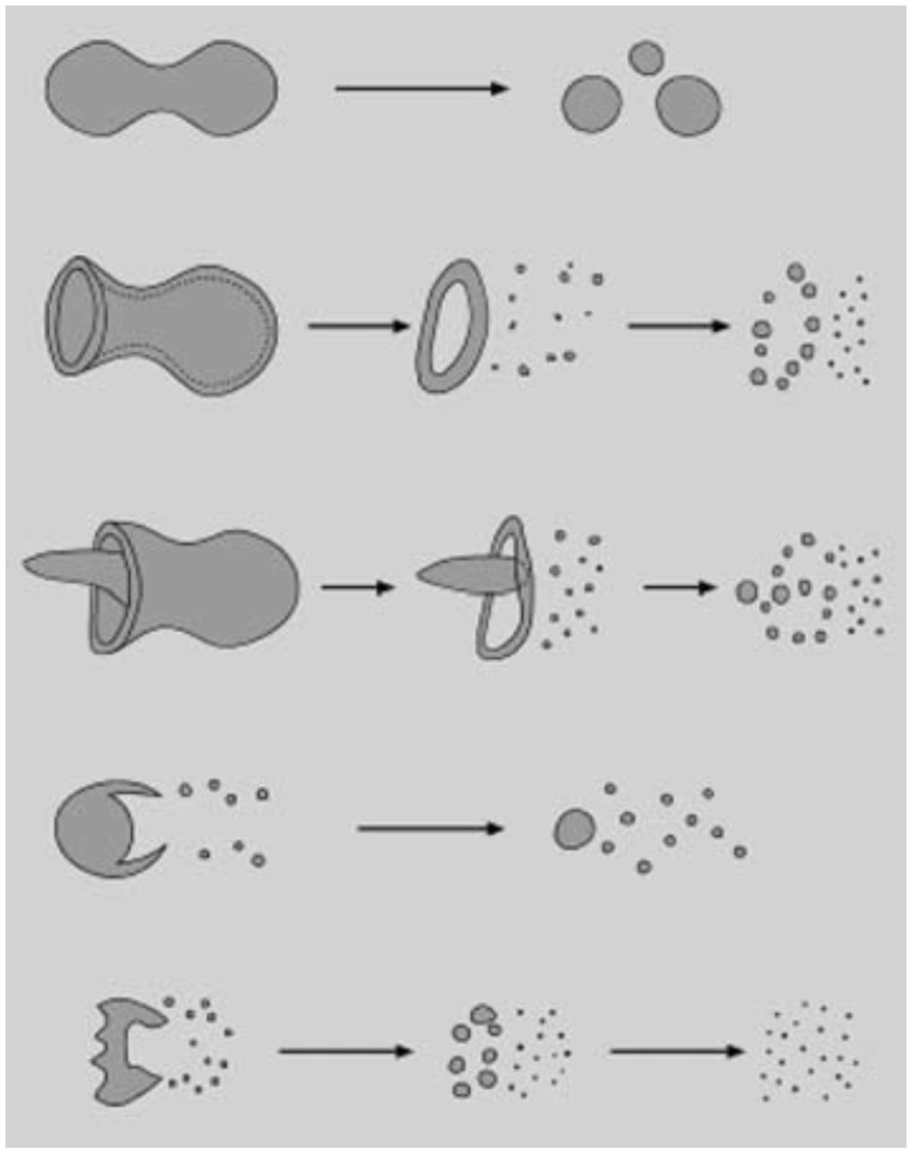
Figure 23.
The secondary breakup morphology of Newtonian drops; from top to bottom, the breakup modes are called vibrational, bag, multimode (often called bag-and-stamen), sheet-thinning, and catastrophic. Reproduced from Reference [259] with permission (Copyright Springer 2009).
Figure 23.
The secondary breakup morphology of Newtonian drops; from top to bottom, the breakup modes are called vibrational, bag, multimode (often called bag-and-stamen), sheet-thinning, and catastrophic. Reproduced from Reference [259] with permission (Copyright Springer 2009).

Table 3.
Transition Weber number for Newtonian drops with Oh < 0.1 [254,261,262].
| Vibrational | 0 < We < ~11 |
|---|---|
| Bag | ~11 < We < ~35 |
| Multimode | ~35 < We < ~80 |
| Sheet-thinning | ~80 < We < ~350 |
| Catastrophic | We > ~350 |
Vibrational breakup consists of oscillation at the drop natural frequency and generates a few fragments with sizes comparable to those of the parent drop [259,261]. As indicated in the work of Pilch and Erdman [262], this breakup mode is not always observed, proceeds much more slowly than other breakup modes, and does not lead to small final fragment sizes. This is why vibrational breakup is ignored, and bag breakup is considered as the first secondary atomization mode by most authors [259]. The geometry of bag breakup includes a thin hollow bag attached to a thicker toroidal rim. The bag disintegrates first, and then the toroidal rim breaks up. Noting that, the bag disintegration results in a larger number of small fragments unlike the toroidal rim disintegration that leads to smaller number of large fragments [259].
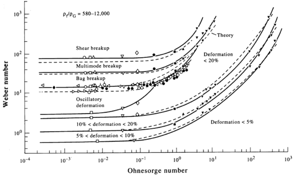
Figure 24.
Secondary breakup regime map. Reproduced from Reference [263] with permission (Copyright Elsevier 1995).
Figure 24.
Secondary breakup regime map. Reproduced from Reference [263] with permission (Copyright Elsevier 1995).

As mentioned above, the bag breakup analysis establishes the criteria for the onset of secondary breakup. The Weber number value that indicates the bag breakup beginning is usually referred to the critical Weber, Wec. When Oh < 0.1, the value for the critical Weber number was reported as Wec = 11 ± 2. For higher Oh conditions, Brodkey [264] suggested the following correlation
where is the critical Weber at low Oh. Pilch and Erdman [262] confirmed the above correlation for Oh < 10. Similarly, Gelfand [265] suggested the following correlation for Oh < 4
Noting that at Oh > 3, the above correlations do not agree with each other [259].
The multimode breakup regime is divided by Dai and Faeth [266] into bag/plume breakup (also named bag-and-stamen) and plume/shear (also called plume/sheet-thinning) breakup. In the bag/plume breakup regime, a bag forms and a plume appears because the center core is blown downstream more slowly [259]. In the Plume/sheet-thinning breakup regime, no bag is formed and drops are stripped continuously from the plume in a way similar to sheet thinning breakup. Dai and Faeth [266] proposed that when Oh < 0.1, the bag/plume breakup occurs for ~18 < We < ~40 and the plume/sheet-thinning occurs for ~40 < We < ~80. Clearly, the mentioned conditions lead to significant overlap with transition We for bag breakup, as given in Table 3. Therefore, it can be concluded that a single transition We value (see Table 3) is an over-simplification and the transition between the breakup modes is essentially a continuous process [259]. In the sheet-thinning or sheet stripping regime, a film is continuously eroded from the drop surface and breaks up rapidly. As a result, a plethora of small droplets and, sometimes, a core with a size that is comparable to that of the parent drop is formed [259]. Hsiang and Faeth [261] found that the drop core might remain at the completion of secondary breakup. In catastrophic breakup, the drop surface is corrugated by large amplitude waves with long wavelengths. These lead to the formation of a small number of large fragments that then disintegrate into smaller units [259].
The total breakup time, Ttot, was defined by Pilch and Erdman [262] as the time when all fragmentation stopped. In the limit of small Oh (for Oh < 0.1), they suggested the following correlations
where
In the above correlation, T is the dimensionless time and t is the dimensional time [259,267]. For the case of viscous drops, Hsiang and Faeth [261] suggested the following correlation
To model the secondary breakup, Taylor Analogy Breakup (TAB), Wave, and Kelvin-Helmholtz Rayleigh-Taylor (KHRT) models are typically used [47]. For low-Weber-number injections (We < 100), the TAB model is suggested. Noting that, the TAB model is based on Taylor’s analogy [268] between an oscillating-distorting drop, and a spring-mass system. Below is the equation for a damped, forced oscillator
where m is the mass, c is the damping coefficient, k is the spring constant, x is the displacement, and F is the force. From Taylor’s analogy, for an oscillating-distorting drop we have
where x is the drop equator displacement from its spherical position, u is the drop relative velocity, σ is the drop surface tension, μl is the drop viscosity, r is the undisturbed drop radius, and ρg and ρl are the gas and liquid phase densities, respectively. In this model, it is assumed that when the distortion grows to a critical ratio of the drop radius, the drop disintegrates. The breakup condition is usually given as 2x > r. In other words, if the distortion is located at the half of the drop radius, the drop breaks up, because the oscillations with this amplitude at the south and north poles meet at the droplet center. By associating the parent droplet energy to the child droplets’ combined energy, the child droplets’ size is determined. The number of child droplets is determined by mass conservation afterwards [47]. The wave model, which was derived from the jet stability analysis [269], is appropriate for high-Weber-number injections (We > 100) and assumes that the resulting droplets’ size and the breakup time are related to the fastest-growing Kelvin-Helmholtz instability [47,269]. In the KHRT model [270], Kelvin-Helmholtz waves effects are combined with Rayleigh-Taylor instabilities. To describe the wave and KHRT formulas in more detail, having at least a fundamental knowledge of stability analysis is necessary. Since explaining the stability theory is beyond the scope of this paper, the interested reader is referred to references [269,270,271] for more information about the secondary breakup models.
4.3. Droplet Evaporation/Combustion
Similar to the suspension atomization, suspension evaporation/combustion within the jets of thermal spray systems is still unknown. Many researchers in the propulsion field have theoretically and experimentally studied the behavior of slurry fuels in high temperature environments. These fuels are very similar to the suspension used in coating technology and are reviewed here. In the propulsion field, slurry fuels include a mixture of liquid hydrocarbon (e.g., ethanol) or water and nano-/micron-sized solid fuel particles (e.g., carbon, aluminum, boron, magnesium or other metals). Most of the time, surfactants are added to the mixture to increase the stability of the suspension [272,273,274]. In general, during the evaporation and combustion of the liquid phase, the particles inside the droplet move and form a shell or crust. Based on the solid particles' melting and boiling points, these particles may even experience a phase change at the shell surface because of exothermic reaction and/or flame radiation [272,273,274].
Generally, the shell properties strongly depend on the solid particle type and size, the base fluid gasification mode and the surfactant composition and concentration [272]. The shell is commonly categorized into three types: rigid and porous, rigid and less porous, and plastic and nonporous (see Figure 25).
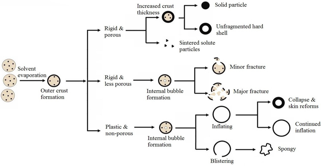
Figure 25.
Shell formation during suspension evaporation/combustion.
Figure 25.
Shell formation during suspension evaporation/combustion.

In the rigid and porous case, there are many pores in the shell and the liquid easily diffuses through them. The liquid vaporization process continues until all liquid is consumed. Therefore, the shell shape does not change and the particle agglomerate remains. In the rigid and less porous case, the diffusion rate of the liquid through the pores decreases due to the shell porosity reduction. The trapped liquid in the core region continues to evaporate and subsequently the pressure in the core region grows. It may result in bubble formation inside the core region and, subsequently, shell fracture. The shell fracture can be minor or major, depending on the porosity level of the shell, and the evaporation rate of the liquid. In the case of a plastic and nonporous shell, the internal pressure growth and bubble formation inside the core region happen. Therefore, the droplet swells and then collapses or becomes spongy [272,273,274]. It has been revealed that the above-mentioned events can happen either separately or jointly [272]. These phenomena have been extensively studied for boron, iron, aluminum, and carbon slurries [272,273,274].
Figure 26 shows the microexplosion phenomenon (bubble formation and fragmentation of the primary droplet) for various slurry droplets, (a) 10 wt % Al nanoparticle (80 nm) in n-decane with 2.5 wt % surfactant; (b) 10 wt % Al micron-sized particle (5 μm) in n-decane with 2.5 wt % surfactant; and (c) 5.0 wt % iron nanoparticle (25 nm) in ethanol without surfactant [273,274]. As can be seen, the microexplosion phenomenon in the case of micron-sized Al suspension (Figure 26b) completely destroys the primary droplet. The difference between the flame characteristics of the nano Al suspension (case (a)) and micron-sized Al suspension (case (b)) is due to their different shell structures. In the nano Al suspension the random Brownian motion of the particles is dominant so that a porous shell is formed. In the micron-sized Al suspension case, the dominant mechanism of the particles’ motion is due to droplet surface regression which forms a densely packed shell. Subsequently, a strong microexplosion happens. In the case of aluminum slurry droplets without using surfactant, there is no microexplosion and particles simply agglomerate after the liquid is fully evaporated. However, for some slurry droplets such as iron/boron in ethanol, a microexplosion happens even without using surfactant (case (c)). The reason can be related to the absorption of water vapor (from the droplet flame and surrounding atmosphere) by the ethanol droplet. Because of water vapor condensation on the ethanol droplet surface, a multicomponent droplet is produced. Since ethanol is more volatile than water, the droplet surface is more concentrated with water. As a result, the ethanol nucleation and bubble formation inside the droplet happens. Then a mild microexplosion happens. It should be noted that the increase of surfactant concentration in slurry droplets increases the intensity of the droplet fragmentation dramatically [273,274]. Carbonization of the surfactant pyrolysis products results in the reduction of shell porosity (carbon atoms bridge the particles).
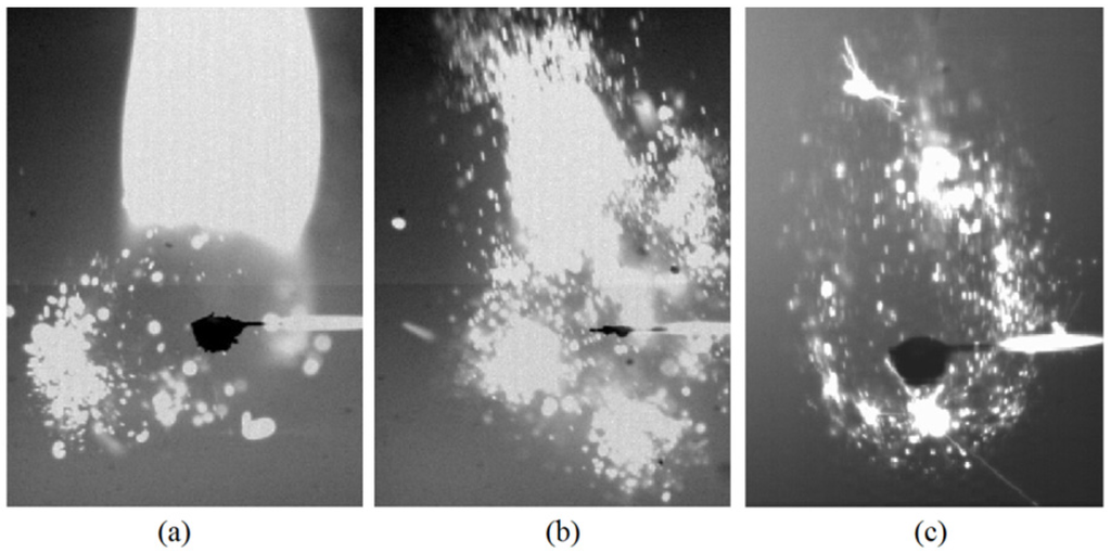
Figure 26.
The combustion and micro-explosion behavior of a slurry fuel droplet with (a) 10 wt % Al nanoparticle (80 nm) in n-decane and 2.5 wt % surfactant; (b) 10 wt % Al micron-sized particle (5 μm) in n-decane and 2.5 wt% surfactant; and (c) 5.0 wt % iron nanoparticle (25 nm) in ethanol without surfactant. Reproduced from References [273,274] with permission (Copyright Elsevier 2011,2012).

In this article, the results of a simple model of single-component droplet evaporation, which are very popular in the field of evaporation and boiling, are presented. For more details of modeling of single-component droplet transient heating and vaporization, multi-component droplet vaporization, and slurry droplet vaporization and combustion, the interested reader is referred to reference [275]. For a single-component droplet, a general and simple correlation for the droplet diameter variation, d, with time, t, (named as d2 law) follows [48]
where d0 is the initial diameter, K is the constant, ρL is the liquid density, KG is the gas thermal conductivity, cpG is the gas specific heat, and hfg is the latent heat of evaporation. The time that takes a droplet with a given initial size to evaporate completely, td, can be found by setting [48]
The droplet vaporization should be simulated when the droplet temperature, Td, is between the vaporization and boiling temperatures (). It can be assumed that the droplet vaporization is controlled by diffusion if its rate is slow [47]
where and are the concentration of vapor in the bulk gas and at the droplet surface, respectively, km is the mass transfer coefficient, and Ni is the vapor molar flux [47]. By equating the vapor partial pressure at the interface to the saturated vapor pressure at the droplet temperature, Psat, the vapor concentration at the droplet surface can be calculated [47]
where Ru is the universal gas constant. Solving the transport equation for species leads to evaluation of the vapor concentration in the bulk gas. To calculate the mass transfer coefficient, the following correlation of the Sherwood number is usually used
where Di,j is the diffusion coefficient, Rep is the droplet Reynolds number, and is the Schmidt number which is the ratio of momentum diffusivity (kinematic viscosity) and mass diffusivity. To calculate the droplet mass reduction, the vapor flux is applied to the droplet mass conservation equation. Moreover, in the gas phase species equation (see Section 2), the vapor flux is considered a source of species i [47].
In addition to vapor diffusion, vapor convection from the droplet surface to the gas phase should be considered if the vaporization rate is high. Miller [276] and Sazhin [277] suggested the following equation for calculating the evaporation rate
where Bm is the Spalding mass number, and are the vapor mass fraction in the bulk gas and at the droplet surface, respectively, md is the droplet mass, and S is the droplet surface area [47]. By changing the droplet heat transfer equation (Equation (8)) to the below equation, the vaporization effect can be considered
When the vaporization rate is high, the following equation can be used to compute the convection heat transfer coefficient
where BT is the Spalding heat transfer number and is usually assumed to be equal to Bm [47].
When the droplet temperature reaches the boiling point, the droplet heat transfer equation becomes
The d2 law is also used to explain the droplet burning lifetime. However, the parameter K is different from Equation (79).
5. Literature Review on HVSFS Modeling
The Eulerian-Lagrangian approach has been used to model the HVSFS process as well. In some preliminary works [278,279,280], the liquid part of the suspension was considered only. The effects of ethanol droplet size, flow rate, and injection velocity on the gas phase and droplet vaporization were studied by Taleby and Hossainpour [278] and Gozali et al. [279]. In the work of Taleby and Hossainpour [278], the premixed combustion of propane-oxygen, the non-premixed combustion of gaseous ethanol-oxygen, and the droplet evaporation were modeled. Both premixed and non-premixed combustions were simulated by the eddy dissipation model. In this study, ethanol was injected axially into the chamber and the droplet breakup simulation was not included. Gozali et al. [279] employed the same approach and simulated the droplet secondary breakup. The droplet breakup for axial injections was modeled by TAB, and for radial injections the wave model was used [279]. Gozali et al. [279] revealed that neglecting modeling droplet breakup results in a high order of errors. They showed that external and radial (into the barrel) injection patterns are not likely appropriate for the HVSFS process as high injection force is demanded [279]. In addition, they showed that the ethanol droplets endure significant disintegration in the middle of the combustion chamber (similar results in [281]) due to the large relative velocity between liquid and gas phases in axial injection pattern. Moreover, it was shown by both teams [278,279] that the liquid feedstock mass flow rate mainly controls the HVSFS process. The maximum evaporation happens inside the combustion chamber which leads to less gas phase cooling and velocity drop if an optimum amount of liquid is injected to the gun.
Gozali et al. [280] developed their model [279] to consider the suspension feedstock as a mixture of water and ethanol. The multicomponent droplets were injected into the combustion chamber axially. For the cases with a high percentage of ethanol in the mixture, the maximum evaporation area takes place inside the combustion chamber. On the other hand, for the cases with high water content in the solvent (more than 50%), the evaporation was considerably delayed and occurred all over the torch internal regions. Droplets experienced severe disintegration in the middle of the combustion chamber and much less effective fragmentation in the barrel and outside the torch. They also concluded that the aqueous solution has a larger influence on the gas dynamics, in contrast to the organic solvent that has less impact on the gas velocity and temperature.
Tabbara and Gu [282] modeled the water droplet injection into a liquid-fueled HVOF torch (JP5000). Liquid kerosene and oxygen were axially injected into the combustion chamber while water droplets were injected into the barrel radially. Both TAB and wave models were applied to simulate the droplet breakup. It was revealed that the droplet fragmentation and evaporation processes are dependent on the initial parent droplet sizes. When the initial diameter of the parent droplet is between 50 and 200 µm, the droplets breakup first and then child droplets vaporize. However, for the parent droplet between 200 and 500 µm, a fraction of the droplets experiences breakup and vaporization simultaneously.
Suspension was considered as two separate parcels in the work of Dongmo et al. [283,284]; droplet (ethanol) and particle (titania) parcels where each parcel was injected into the combustion chamber axially. To simulate the ethanol vapor flame (the non-premixed combustion), the finite rate chemistry model in Arrhenius form was used. In addition, the eddy dissipation model was used to simulate the premixed (propane/oxygen) combustion. They showed that the injection angle variation has a significant influence on the ethanol residence time and evaporation length in the combustion chamber. Furthermore, by changing the straight geometry of the combustion chamber to a conical shape, they achieved good results regarding the micron and nanoparticle trajectories in the combustion chamber.
Jabbari et al. [50] used a two-component mixture model for simulating the suspension with a given particle concentration as a slurry droplet. The main goal was to mimic the suspension breakup, vaporization, particle temperature, velocity, and trajectory in the suspension plasma spraying. The first component was the base fluid (e.g., ethanol), and the second component was considered to have the same properties as nickel (density, evaporation temperature, latent heat of evaporation, etc.). To determine the coating particles’ characteristics, the suspended particles were tracked after completion of the suspension breakup and vaporization (see Figure 27 and Figure 28). This model was used by Jadidi et al. [285] and Pourang et al. [286] to investigate the effect of substrate shape and curvature on in-flight particle velocity, temperature, and trajectory in suspension plasma spraying (see Figure 27 and Figure 28). The mentioned approach yielded reasonable results regarding droplet/particle in-flight behavior and can be used to model the HVSFS process.

Figure 27.
The droplet/particle temperature and trajectory in suspension plasma spray at different standoff distances (D). Reproduced from Reference [285] with permission (Copyright Springer 2015).
Figure 27.
The droplet/particle temperature and trajectory in suspension plasma spray at different standoff distances (D). Reproduced from Reference [285] with permission (Copyright Springer 2015).
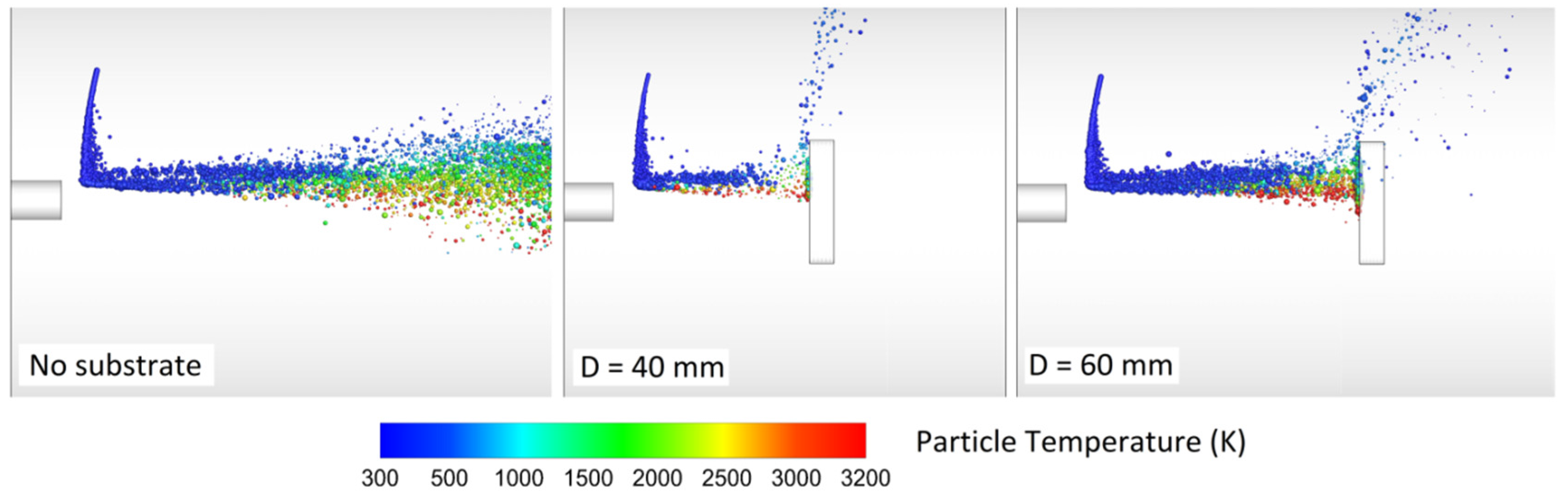

Figure 28.
The droplet/particle velocity and trajectory in suspension plasma spray at different standoff distances (D). Reproduced from Reference [285] with permission (Copyright Springer 2015).
Figure 28.
The droplet/particle velocity and trajectory in suspension plasma spray at different standoff distances (D). Reproduced from Reference [285] with permission (Copyright Springer 2015).
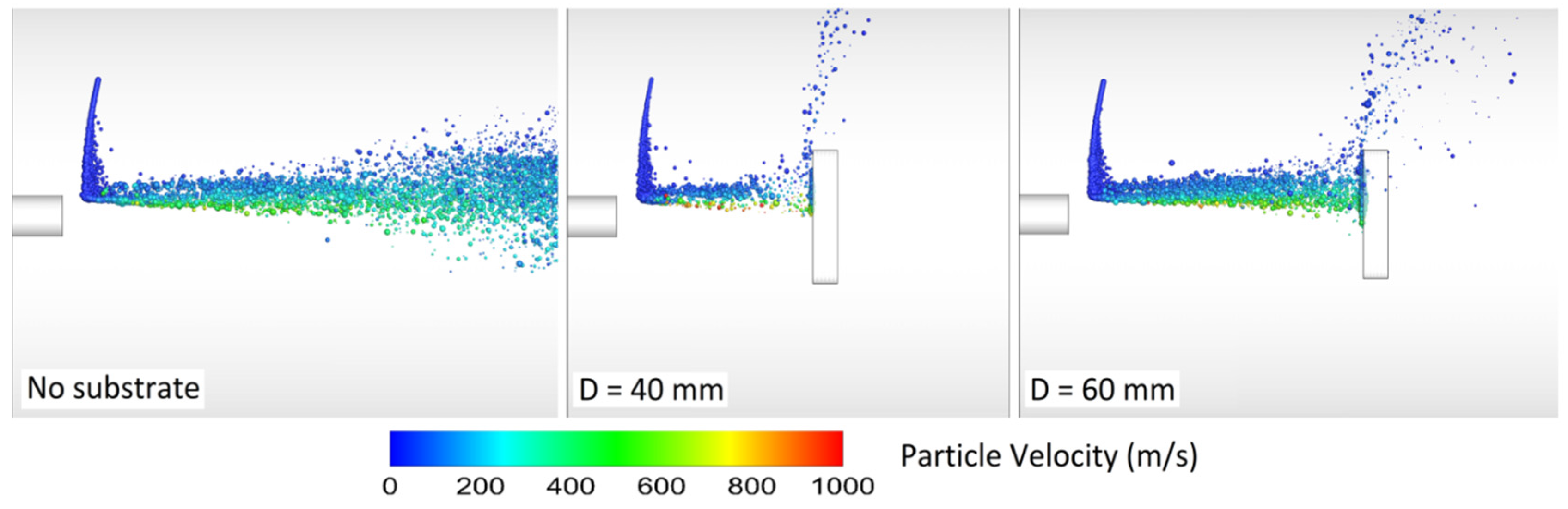
6. Conclusions and Future Works
As mentioned, many different fields such as gas/droplet/solid/slurry fuel combustion, crossflow/co-flow atomization, two-/three-phase flow gas dynamics, two-/three-phase compressible flow, turbulent flow, suspension, and nanofluid are involved in thermal spray processes. Therefore, numerical modeling of thermal sprays is very challenging. In this paper, a comprehensive review on the fundamental phenomena involved in the thermal sprays, especially HVOF and HVSFS processes, is presented. Moreover, pros and cons of the most popular numerical methods in this field such as the Eulerian-Lagrangian approach and the volume of fluid method are discussed in this article. Accurate empirical correlations for drag and thermophoretic forces, Nusselt number, atomization characteristics, and suspension properties are presented. In addition, a comprehensive review on simulation results published to date is provided.
It is also mentioned that suspension/liquid injection into the plasma/HVOF spray torches has recently attracted much attention due to the superior performance of the produced coatings. In addition, many parameters and mechanisms, especially in the suspension spraying and liquid-fueled HVOF torches, are unknowns and need to be understood for further advancement of the process. In order to fully exploit this emerging process, the effect of suspension flow rate, suspension properties, injector angle, axial and radial injection, spray atomization and injection of continuous jets, substrate shape, and location on the coatings can be simulated. Briefly, to simulate and understand the mechanisms involved in the suspension thermal spray and to control and improve the coating quality, the following steps are suggested.
- Coupling of level set (LS) and volume of fluid (VOF) methods to simulate both inertia-dominated and surface tension-dominated compressible multiphase flows (the CLSVOF method);
- Coupling the mentioned fully Eulerian methods such as CLSVOF and Lagrangian spray models to simulate both primary and secondary atomization;
- After secondary atomization modeling, tracking the droplets/particles in the domain using the Eulerian-Lagrangian approach;
- Using more accurate turbulence models such as large eddy simulation (LES);
- Measuring and correlating suspension properties, especially dynamic and static surface tensions (these parameters has significant effects on the atomization process);
- Understanding the suspension evaporation/combustion mechanisms within the high temperature jets and flames (they have some influence on the particle agglomerations' sizes and, subsequently, on the adhesion of the coating on the substrate);
- Considering the effect of the Knudsen number on the Nusselt number and heat transfer coefficient;
- Considering the thermophoretic force;
- Parametric study to optimize the torch;
- The effect of Weber, Ohnesorge, and Reynolds numbers on the atomization process and droplet size distribution in HVOF torches;
- The effect of suspension/liquid injector shape, type, and location on the droplet size distribution and droplet velocity in HVOF torches;
- The effect of operating conditions such as total flow rate and equivalence ratio on the atomization process and droplet combustion;
- The effect of combustion chamber geometry and injector angle on the droplet size distribution, droplet velocity, droplet combustion, and particle temperature and velocity;
- The effect of torch geometry on the particle temperature and oxidation;
- The effect of standoff distance and substrate shape on the deposition efficiency.
Finally, finding the optimum torch geometry and operating conditions.
Acknowledgments
The authors would like to acknowledge the support provided by Natural Sciences and Engineering Research Council of Canada (NSERC).
Conflicts of Interest
The authors declare no conflict of interest.
References
- Pawlowski, L. The Science and Engineering of Thermal Spray Coatings, 2nd ed.; John Wiley & Sons: Chichester, West Sussex, UK, 2008. [Google Scholar]
- Heimann, R.B. Plasma Spray Coating: Principles and Applications, 2nd ed.; Wiley-VCH Verlagsgesellschaft mbH: Weinheim, Germany, 1996. [Google Scholar]
- Sobolev, V.V.; Guilemany, J.M.; Nutting, J. High Velocity Oxy-Fuel Spraying: Theory, Structure-Property Relationships and Applications; Maney Publishing: London, UK, 2004. [Google Scholar]
- Li, M.; Christofides, P.D. Modeling and control of high-velocity oxygen-fuel (HVOF) thermal spray: A tutorial review. J. Therm. Spray Technol. 2009, 18, 753–768. [Google Scholar] [CrossRef]
- Cetegen, B.M.; Basu, S. Review of modeling of liquid precursor droplets and particles injected into plasmas and high-velocity oxy-fuel (HVOF) flame jets for thermal spray deposition applications. J. Therm. Spray Technol. 2009, 18, 769–793. [Google Scholar] [CrossRef]
- Oksa, M.; Turunen, E.; Suhonen, T.; Varis, T.; Hannula, S.P. Optimization and characterization of high velocity oxy-fuel sprayed coatings: Techniques, materials, and applications. Coatings 2011, 1, 17–25. [Google Scholar] [CrossRef]
- Fauchais, P.; Montavon, G.; Lima, R.S.; Marple, B.R. Engineering a new class of thermal spray nano-based microstructures from agglomerated nanostructured particles, suspensions and solutions: An invited review. J. Phys. D Appl. Phys. 2011, 44. [Google Scholar] [CrossRef]
- Dolatabadi, A. A Computational Analysis of High Speed Particle-Laden Flows. Ph.D. Thesis, University of Toronto, Toronto, ON, Canada, 2003. [Google Scholar]
- Gu, S.; McCartney, D.G.; Eastwick, C.N.; Simmons, K.A. Numerical modeling of in-flight characteristics of Inconel 625 particles during high-velocity oxy-fuel thermal spraying. J. Therm. Spray Technol. 2004, 13, 200–213. [Google Scholar] [CrossRef]
- Law, C.K. Combustion physics; Cambridge University Press: Cambridge, UK, 2006. [Google Scholar]
- Kobayashi, H.; Nakashima, T.; Tamura, T.; Maruta, K.; Niioka, T. Turbulence measurements and observations of turbulent premixed flames at elevated pressures up to 3.0 MPa. Combust. Flame 1997, 108, 104–117. [Google Scholar] [CrossRef]
- Kobayashi, H.; Tamura, T.; Maruta, K.; Niioka, T.; Williams, F.A. Burning velocity of turbulent premixed flames in a high-pressure environment. In Proceedings of the 26th Symposium (International) on Combustion, Naples, Italy, 28 July–2 August 1996; pp. 389–396.
- Kobayashi, H.; Kawabata, Y.; Maruta, K. Experimental study on general correlation of turbulent burning velocity at high pressure. In Proceedings of the 27th Symposium (International) on Combustion, Boulder, CO, USA, 2–7 August 1998; pp. 941–948.
- Kobayashi, H. Experimental study of high-pressure turbulent premixed flames. Exp. Therm. Fluid Sci. 2002, 26, 375–387. [Google Scholar] [CrossRef]
- Norman, M.L.; Winkler, K.A. Supersonic Jets. In Los Alamos Science; Los Alamos Science Center: Los Alamos National Laboratory, NM, USA, 1985. [Google Scholar]
- Anderson, J.D., Jr. Modern Compressible Flow with Historical Perspective, 2nd ed.; McGraw-Hill: Singapore, Singapore, 1990. [Google Scholar]
- Aerospaceweb. Available online: http://www.aerospaceweb.org/question/propulsion/q0224.shtml (accessed on 14 August 2015).
- Munday, D.; Gutmark, E.; Liu, J.; Kailasanath, K. Flow structure and acoustics of supersonic jets from conical convergent-divergent nozzles. Phys. Fluids 2011, 23. [Google Scholar] [CrossRef]
- Samareh, B.; Stier, O.; Luthen, V.; Dolatabadi, A. Assessment of CFD modeling via flow visualization in cold spray process. J. Therm. Spray Technol. 2009, 18, 934–943. [Google Scholar] [CrossRef]
- Andreopoulos, Y.; Agui, J.H.; Briassulis, G. Shock wave-turbulence interactions. Annu. Rev. Fluid Mech. 2000, 32, 309–345. [Google Scholar] [CrossRef]
- Garnier, E.; Adams, N.; Sagaut, P. Large Eddy Simulation for Compressible Flows; Springer: New York, NY, USA, 2009. [Google Scholar]
- Fan, L.S.; Zhu, C. Principles of Gas-Solid Flows; Cambridge University Press: Cambridge, UK, 1998. [Google Scholar]
- Rudinger, G. Relaxation in Gas-Particle Flow. Project SQUID; Technical Report No. CAL-96-PU; July 1968. [Google Scholar]
- Varma, T.D.; Chopra, N.K. Analysis of normal shock waves in a gas-particle mixture. Z. Angew. Math. Phys. 1967, 18, 650–660. [Google Scholar] [CrossRef]
- Srivastava, R.S.; Sharma, J.P. Structure of normal shock waves in a gas-particle mixture. Z. Angew. Math. Phys. 1982, 33, 819–825. [Google Scholar] [CrossRef]
- John, E.A.; Keith, T.G. Gas. Dynamics, 3rd ed.; Pearson Prentice Hall: Upper Saddle River, NJ, USA, 2006. [Google Scholar]
- Crowe, C.; Sommerfeld, M.; Tsuji, Y. Multiphase Flows with Droplets and Particles; CRC Press: Boca Raton, FL, USA, 1998. [Google Scholar]
- Berry, R.A. Ensemble Averaged Conservation Equations for Multiphase, Multi-Component, and Multi-Material Flows. In Idaho National Engineering and Environmental Laboratory, Bechtel BWXT Idaho, INEEL/EXT-03–01011; Idaho National Laboratory: Idaho Falls, ID, USA, 2003. [Google Scholar]
- Kashiwa, B.A.; Rauenzahn, R.M. A Multimaterial Formalism; Technical Report LA-UR-94-771; Los Alamos National Laboratory: Los Alamos, NM, USA, 1994. [Google Scholar]
- Elghobashi, S.E. On predicting particle-laden turbulent flows. Appl. Sci. Res. 1994, 52, 309–329. [Google Scholar] [CrossRef]
- Dolatabadi, A.; Mostaghimi, J.; Pershin, V. Modeling dense suspension of solid particles in highly compressible flows. Int. J. Comput. Fluid Dyn. 2004, 18, 125–131. [Google Scholar] [CrossRef]
- Samareh, B.; Dolatabadi, A. Dense particulate flow in a cold gas dynamic spray system. J. Fluids Eng. 2008, 130. [Google Scholar] [CrossRef]
- Crowe, C.T. Drag coefficient on particles in a rocket nozzle. AIAA J. 1967, 5, 1021–1022. [Google Scholar] [CrossRef]
- Clift, R.; Grace, J.R.; Weber, M.E. Bubbles, Drops and Particles; Academic Press: New York, NY, USA, 1978. [Google Scholar]
- Samareh Abolhassani, B. Two phase flow modeling of cold spray process. Master’s Thesis, Concordia University, Montreal, QC, Canada, 2008. [Google Scholar]
- Siegel, R.; Howell, J.R. Thermal radiation heat transfer, 2nd ed.; Hemisphere Publishing Corp: Washington, DC, USA, 1981. [Google Scholar]
- Li, M.; Shi, D.; Christofides, P.D. Modeling and control of HVOF thermal spray processing of WC-Co coatings. Powder Technol. 2005, 156, 177–194. [Google Scholar] [CrossRef]
- Viskanta, R.; Menguc, M.P. Radiation heat transfer in combustion systems. Prog. Energy Combust. Sci. 1987, 13, 97–160. [Google Scholar] [CrossRef]
- Bohren, C.F.; Huffman, D.R. Absorption and Scattering of Light by Small Particles; Wiley: New York, NY, USA, 1983. [Google Scholar]
- Van de Hulst, H.C. Light Scattering by Small Particles; Wiley: New York, NY, USA, 1957. [Google Scholar]
- Wickramasinghe, N.C. Light Scattering Functions for Small Particles; Wiley: New York, NY, USA, 1973. [Google Scholar]
- Jones, A.R. Light scattering for particle characterization. Prog. Energy Combust. Sci. 1999, 25, 1–53. [Google Scholar] [CrossRef]
- Ordal, M.A.; Long, L.L.; Bell, R.J.; Bell, S.E.; Bell, R.R.; Alexander, R.W.; Ward, C.A. Optical properties of the metals Al, Co, Cu, Au, Fe, Pb, Ni, Pd, Pt, Ag, Ti, and W in the infrared and far infrared. Appl. Opt. 1983, 22, 1099–1119. [Google Scholar] [CrossRef] [PubMed]
- Bidabadi, M.; Shabani Shahrbabaki, A.; Jadidi, M.; Montazerinejad, S. An analytical study of radiation effect on the premixed laminar flame of aluminum dust clouds. Proc. Inst. Mech. Eng. Part C J. Mech. Eng. Sci. 2010, 224, 1679–1695. [Google Scholar] [CrossRef]
- Plass, G.N. Mie scattering and absorption cross sections for aluminum oxide and magnesium oxide. Appl. Opt. 1964, 3, 867–872. [Google Scholar] [CrossRef]
- Echekki, T.; Mastorakos, E. Turbulent Combustion Modeling, Advances, New Trends and Perspectives; Springer: Dordrecht, The Netherlands, 2010. [Google Scholar]
- ANSYS FLUENT Theory Guide; Release 14.0; ANSYS, Inc.: Cecil Township, PA, USA, 2011.
- Turns, S.R. An Introduction to Combustion, Concepts and Applications, 2nd ed.; McGraw-Hill: New York, NY, USA, 2000. [Google Scholar]
- Glassman, I.; Yetter, R.A. Combustion, 4th ed.; Academic Press: Burlington, MA, USA, 2008. [Google Scholar]
- Jabbari, F.; Jadidi, M.; Wuthrich, R.; Dolatabadi, A. A numerical study of suspension injection in plasma spraying process. J. Therm. Spray Technol. 2014, 23, 3–13. [Google Scholar] [CrossRef]
- Marchand, C.; Chazelas, C.; Mariaux, G.; Vardelle, A. Liquid precursor plasma spraying: Modeling the interactions between the transient plasma jet and the droplets. J. Therm. Spray Technol. 2007, 16, 705–712. [Google Scholar] [CrossRef]
- Vincent, S.; Balmigere, G.; Caruyer, C.; Meillot, E.; Caltagirone, J.P. Contribution to the modeling of the interaction between a plasma flow and a liquid jet. Surf. Coat. Technol. 2009, 203, 2162–2171. [Google Scholar] [CrossRef]
- Caruyer, C.; Vincent, S.; Meillot, E.; Caltagirone, J.P. Modeling the first instant of the interaction between a liquid and a plasma jet with a compressible approach. Surf. Coat. Technol. 2010, 205, 974–979. [Google Scholar] [CrossRef]
- Caruyer, C.; Vincent, S.; Meillot, E.; Caltagirone, J.P.; Damiani, D. Analysis of the unsteadiness of a plasma jet and the related turbulence. Surf. Coat. Technol. 2010, 205, 1165–1170. [Google Scholar] [CrossRef]
- Cheng, C.H.; Moore, R.L. Numerical simulation of gas and particle flow in a high velocity oxygen-fuel (HVOF) torch. J. Therm. Spray Technol. 1995, 4, 358–366. [Google Scholar] [CrossRef]
- Oberkampf, W.L.; Talpallikar, M. Analysis of High Velocity Oxygen Fuel (HVOF) Thermal Spray Torch, Part 1: Numerical formulation. In Proceedings of the 7th National Thermal Spray Conference, Boston, MA, USA, 20–24 June 1994; pp. 381–386.
- Oberkampf, W.L.; Talpallikar, M. Analysis of High Velocity Oxygen Fuel (HVOF) Thermal Spray Torch, Part 2: Computational Results. In Proceedings of the 7th National Thermal Spray Conference, Boston, MA, USA, 20–24 June 1994; pp. 387–392.
- Hassan, B.; Oberkampf, W.L.; Neiser, R.A.; Roemer, T.J. Computational fluid dynamics analysis of a high-velocity oxygen-fuel (HVOF) thermal spray torch. In Proceedings of the 8th National Thermal Spray Conference, Houston, TX, USA, 11–15 September 1995.
- Westbrook, C.K.; Dryer, F.L. Simplified reaction mechanisms for the oxidation of hydrocarbon fuels in flames. Combust. Sci. Technol. 1981, 27, 31–43. [Google Scholar] [CrossRef]
- Li, M.; Christofides, P.D. Multi-scale modeling and analysis of an industrial HVOF thermal spray process. Chem. Eng. Sci. 2005, 60, 3649–3669. [Google Scholar] [CrossRef]
- Hossainpour, S.; Binesh, A.R. A CFD study of sensitive parameters effect on the combustion in a high velocity oxygen-fuel thermal spray gun. Proc. World Acad. Sci. Eng. Technol. 2008, 41, 213–220. [Google Scholar]
- Kamali, R.; Binesh, A.R. The importance of sensitive parameters effect on the combustion in a high velocity oxygen-fuel spray system. Int. Commun. Heat Mass Transf. 2009, 36, 978–983. [Google Scholar] [CrossRef]
- Dolatabadi, A.; Mostaghimi, J.; Pershin, V. Effect of a cylindrical shroud on particle conditions in high velocity oxy-fuel spray process. Sci. Technol. Adv. Mater. 2002, 3, 245–255. [Google Scholar] [CrossRef]
- Dolatabadi, A.; Mostaghimi, J.; Pershin, V. Effect of a cylindrical shroud on particle conditions in high velocity oxy-fuel (HVOF) spray process. J. Mater. Process. Technol. 2003, 137, 214–224. [Google Scholar] [CrossRef]
- Srivatsan, V.R.; Dolatabadi, A. Simulation of particle-shock interaction in a high velocity oxygen fuel process. J. Therm. Spray Technol. 2006, 15, 481–487. [Google Scholar] [CrossRef]
- Kamnis, S.; Gu, S. Numerical modeling of propane combustion in a high velocity oxygen-fuel thermal spray gun. Chem. Eng. Process. 2006, 45, 246–253. [Google Scholar] [CrossRef]
- Kamnis, S.; Gu, S. 3-D modeling of kerosene-fuelled HVOF thermal spray gun. Chem. Eng. Sci. 2006, 61, 5427–5439. [Google Scholar] [CrossRef]
- Tabbara, H.; Gu, S. Computational simulation of liquid-fuelled HVOF thermal spraying. Surf. Coat. Technol. 2009, 204, 676–684. [Google Scholar] [CrossRef]
- Dongmo, E.; Wenzelburger, M.; Gadow, R. Analysis and optimization of the HVOF process by combined experimental and numerical approaches. Surf. Coat. Technol. 2008, 202, 4470–4478. [Google Scholar] [CrossRef]
- Kadyrov, E.; Evdokimenko, Y.; Kisel, V.; Kadyrov, V.; Worzala, F. Interaction of particles with carrier gas in HVOF spraying systems. J. Therm. Spray Technol. 1994, 3, 389–397. [Google Scholar] [CrossRef]
- Cheng, D.; Xu, Q.; Trapaga, G.; Lavernia, E.J. A numerical study of high-velocity oxygen fuel thermal spraying process, part I: Gas phase dynamics. Metall. Mater. Trans. A 2001, 32A, 1609–1620. [Google Scholar] [CrossRef]
- Li, M.; Christofides, P.D. Modeling and analysis of HVOF thermal spray process accounting for powder size distribution. Chem. Eng. Sci. 2003, 58, 849–857. [Google Scholar] [CrossRef]
- Li, M.; Shi, D.; Christofides, P.D. Diamond jet hybrid HVOF thermal spray: Gas-phase and particle behavior modeling and feedback control design. Ind. Eng. Chem. Res. 2004, 43, 3632–3652. [Google Scholar] [CrossRef]
- Gu, S.; Eastwick, C.N.; Simmons, K.A.; McCartney, D.G. Computational fluid dynamic modeling of gas flow characteristics in a high-velocity oxy-fuel thermal spray system. J. Therm. Spray Technol. 2001, 10, 461–469. [Google Scholar]
- Yang, X.; Eidelman, S. Numerical analysis of a high velocity oxygen-fuel thermal spray system. J. Therm. Spray Technol. 1996, 5, 175–184. [Google Scholar] [CrossRef]
- Joshi, S.V.; Sivakumar, R. Particle behaviour during high velocity oxy-fuel spraying. Surf. Coat. Technol. 1991, 50, 67–74. [Google Scholar] [CrossRef]
- Joshi, S.V. A prediction model to assist plasma and HVOF spraying. Mater. Lett. 1992, 14, 31–36. [Google Scholar] [CrossRef]
- Sobolev, V.V.; Guilemany, J.M.; Garmier, J.C.; Calero, J.A. Modeling of particle movement and thermal behaviour during high velocity oxy-fuel spraying. Surf. Coat. Technol. 1994, 63, 181–187. [Google Scholar] [CrossRef]
- Sobolev, V.V.; Guilemany, J.M.; Miguel, J.R.; Calero, J.A. Influence of in-flight dissolution process on composite powder particle (WC-Ni) behaviour during high velocity oxy-fuel spraying. Surf. Coat. Technol. 1996, 81, 136–145. [Google Scholar] [CrossRef]
- Sobolev, V.V.; Guilemany, J.M.; Martin, A.J.; Calero, J.A. Modeling of the in-flight behaviour of the stainless steel powder particles in high velocity oxy-fuel spraying. J. Mater. Process. Technol. 1998, 79, 213–216. [Google Scholar] [CrossRef]
- Ait-Messaoudene, N.; Abdellah El-hadj, A. Effect of the substrate and of thermophoresis on the acceleration and heating of particles during HVOF spraying. Surf. Coat. Technol. 1998, 106, 140–144. [Google Scholar] [CrossRef]
- Cheng, D.; Xu, Q.; Trapaga, G.; Lavernia, E.J. The effect of particle size and morphology on the in-flight behavior of particles during high-velocity oxyfuel thermal spraying. Metall. Mater. Trans. B 2001, 32B, 525–535. [Google Scholar] [CrossRef]
- Ganser, G.H. A rational approach to drag prediction of spherical and nonspherical particles. Powder Technol. 1993, 77, 143–152. [Google Scholar] [CrossRef]
- Gu, S.; Kamnis, S. Numerical modeling of in-flight particle dynamics of non-spherical powder. Surf. Coat. Technol. 2009, 203, 3485–3490. [Google Scholar] [CrossRef]
- Kamnis, S.; Gu, S. Study of in-flight and impact dynamics of nonspherical particles from HVOF guns. J. Therm. Spray Technol. 2010, 19, 31–41. [Google Scholar] [CrossRef]
- Hackett, C.M.; Settles, G.S. The influence of nozzle design on HVOF spray particle velocity and temperature. In Proceedings of 8th National Thermal Spray Conference, Houston, TX, USA, 11–15 September 1995.
- Li, M.; Christofides, P.D. Computational study of particle in-flight behavior in the HVOF thermal spray process. Chem. Eng. Sci. 2006, 61, 6540–6552. [Google Scholar] [CrossRef]
- Lopez, A.R.; Hassan, B.; Oberkampf, W.L.; Neiser, R.A.; Roemer, T.J. Computational fluid dynamics analysis of a wire-feed high-velocity oxygen fuel (HVOF) thermal spray torch. J. Therm. Spray Technol. 1998, 7, 374–382. [Google Scholar] [CrossRef]
- Kamnis, S.; Gu, S.; Zeoli, N. Mathematical modeling of Inconel 718 particles in HVOF thermal spraying. Surf. Coat. Technol. 2008, 202, 2715–2724. [Google Scholar] [CrossRef]
- Kamnis, S.; Gu, S.; Lu, T.J.; Chen, C. Computational simulation of thermally sprayed WC-Co powder. Comput. Mater. Sci. 2008, 43, 1172–1182. [Google Scholar] [CrossRef]
- Katanoda, H.; Yamamoto, H.; Matsuo, K. Numerical simulation on supersonic flow in high-velocity oxy-fuel thermal spray gun. J. Therm. Sci. 2006, 15, 65–70. [Google Scholar] [CrossRef]
- Katanoda, H. Quasi-one dimensional analysis of the effects of pipe friction, cooling and nozzle geometry on gas/particle flows in HVOF thermal spray gun. Mater. Trans. 2006, 47, 2791–2797. [Google Scholar] [CrossRef] [Green Version]
- Hassan, B.; Lopez, A.R.; Oberkampf, W.L. Computational analysis of a three-dimensional high-velocity oxygen fuel (HVOF) thermal spray torch. J. Therm. Spray Technol. 1998, 7, 71–77. [Google Scholar] [CrossRef]
- Zeoli, N.; Gu, S.; Kamnis, S. Numerical simulation of in-flight particle oxidation during thermal spraying. Comput. Chem. Eng. 2008, 32, 1661–1668. [Google Scholar] [CrossRef]
- Neiser, R.A.; Smith, M.F.; Dykhuizen, R.C. Oxidation in wire HVOF sprayed steel. J. Therm. Spray Technol. 1998, 7, 537–545. [Google Scholar] [CrossRef]
- Dobler, K.; Kreye, H.; Schwetzke, R. Oxidation of stainless steel in the high velocity oxy-fuel process. J. Therm. Spray Technol. 2000, 9, 407–413. [Google Scholar] [CrossRef]
- Sakaki, K.; Shimizu, Y. Effect of the increase in the entrance convergent section length of the gun nozzle on the high-velocity oxygen fuel and cold spray process. J. Therm. Spray Technol. 2001, 10, 487–496. [Google Scholar] [CrossRef]
- Baik, J.S.; Kim, Y.J. Effect of nozzle shape on the performance of high velocity oxygen-fuel thermal spray system. Surf. Coat. Technol. 2008, 202, 5457–5462. [Google Scholar] [CrossRef]
- Kim, S.H.; Kim, Y.J. Flow characteristics in compact thermal spray coating systems with minimum length nozzle. Plasma Sci. Technol. 2009, 11, 550–554. [Google Scholar] [CrossRef]
- Dolatabadi, A.; Pershin, V.; Mostaghimi, J. New attachment for controlling gas flow in the HVOF process. J. Therm. Spray Technol. 2005, 14, 91–99. [Google Scholar] [CrossRef]
- Dai, S.L.; Delplanque, J.P.; Lavernia, E.J. Microstructural characteristics of 5083 Al alloys processed by reactive spray deposition for net-shape manufacturing. Metall. Mater. Trans. A 1998, 29, 2597–2611. [Google Scholar] [CrossRef]
- Haider, A.; Levenspiel, O. Drag coefficient and terminal velocity of spherical and nonspherical particles. Powder Technol. 1989, 58, 63–70. [Google Scholar] [CrossRef]
- Eidelman, S.; Yang, X. Three dimensional simulation of HVOF spray deposition of nanoscale materials. Nanostruct. Mater. 1997, 9, 79–84. [Google Scholar] [CrossRef]
- Ma, M.; Hill, R.M. Superhydrophobic surfaces. Curr. Opin. Colloid Interface Sci. 2006, 11, 193–202. [Google Scholar] [CrossRef]
- Nosonovsky, M.; Bhushan, B. Superhydrophobic surfaces and emerging applications: Non-adhesion, energy, green engineering. Curr. Opin. Colloid Interface Sci. 2009, 14, 270–280. [Google Scholar] [CrossRef]
- Bhushan, B.; Jung, Y.C. Natural and biomimetic artificial surfaces for superhydrophobicity, self-cleaning, low adhesion, and drag reduction. Prog. Mater. Sci. 2011, 56, 1–108. [Google Scholar] [CrossRef]
- Moghtadernejad, S.; Tembely, M.; Jadidi, M.; Esmail, N.; Dolatabadi, A. Shear driven droplet shedding and coalescence on a superhydrophobic surface. Phys. Fluids 2015, 27. [Google Scholar] [CrossRef]
- Moghtadernejad, S.; Jadidi, M.; Tembely, M.; Esmail, N.; Dolatabadi, A. Concurrent droplet coalescence and solidification on surfaces with various wettabilities. J. Fluids Eng. 2015, 137. [Google Scholar] [CrossRef]
- Moghtadernejad, S.; Mohammadi, M.; Jadidi, M.; Tembely, M.; Dolatabadi, A. Shear driven droplet shedding on surfaces with various wettabilities. SAE Int. J. Aerosp. 2013, 6, 459–464. [Google Scholar] [CrossRef]
- Moghtadernejad, S.; Jadidi, M.; Esmail, N.; Dolatabadi, A. Shear driven droplet coalescence and rivulet formation. Proc. Inst. Mech. Engrs. Part. C J. Mech. Engng. Sci. 2015, in press. [Google Scholar] [CrossRef]
- Moghtadernejad, S. Dynamics of Droplet Shedding and Coalescence under the Effect of Shear Flow. Ph.D. Thesis, Concordia University, Montreal, QC, Canada, 2014. [Google Scholar]
- Moghtadernejad, S.; Jadidi, M.; Esmail, N.; Dolatabadi, A. SPH simulation of rivulet dynamics on surfaces with various wettabilities. SAE Int. J. Aerosp. 2015. in Press. [Google Scholar] [CrossRef]
- Moghtadernejad, S.; Jadidi, M.; Tembely, M.; Dolatabadi, A. Shear driven rivulet dynamics on surfaces with various wettabilities. In Proceedings of the ASME 2014 International Mechanical Engineering Congress and Exposition, Montreal, QC, Canada, 14–20 November 2014.
- Aghasibeig, M.; Mousavi, M.; Ben Ettouill, F.; Moreau, C.; Wuthrich, R.; Dolatabadi, A. Electrocatalytically active nickel-based electrode coatings formed by atmospheric and suspension plasma spraying. J. Therm. Spray Technol. 2014, 23, 220–226. [Google Scholar] [CrossRef]
- Pawlowski, L. Suspension and solution thermal spray coatings. Surf. Coat. Technol. 2009, 203, 2807–2829. [Google Scholar] [CrossRef]
- Toma, F.L.; Berger, L.M.; Jacquet, D.; Wicky, D.; Villaluenga, I.; de Miguel, Y.R.; Lindelov, J.S. Comparative study on the photocatalytic behavior of titanium oxide thermal sprayed coatings from powders and suspensions. Surf. Coat. Technol. 2009, 203, 2150–2156. [Google Scholar] [CrossRef]
- Killinger, A.; Kuhn, M.; Gadow, R. High-velocity suspension flame spraying (HVSFS), a new approach for spraying nanoparticles with hypersonic speed. Surf. Coat. Technol. 2006, 201, 1922–1929. [Google Scholar] [CrossRef]
- Fazilleau, J.; Delbos, C.; Rat, V.; Coudert, J.F.; Fauchais, P.; Pateyron, B. Phenomena involved in suspension plasma spraying part 1: Suspension injection and behavior. Plasma Chem. Plasma Process 2006, 26, 371–391. [Google Scholar] [CrossRef]
- Fauchais, P.; Montavon, G.; Bertrand, G. From powders to thermally sprayed coatings. J. Therm. Spray Technol. 2010, 19, 56–80. [Google Scholar] [CrossRef]
- Gadow, R.; Killinger, A.; Rauch, J. Introduction to high-velocity suspension flame spraying (HVSFS). J. Therm. Spray Technol. 2008, 17, 655–661. [Google Scholar] [CrossRef]
- Yu, W.; France, D.M.; Routbort, J.L.; Choi, S.U.S. Review and comparison of nanofluid thermal conductivity and heat transfer enhancements. Heat Transfer Eng. 2008, 29, 432–460. [Google Scholar] [CrossRef]
- Ghadimi, A.; Saidur, R.; Metselaar, H.S.C. A review of nanofluid stability properties and characterization in stationary conditions. Int. J. Heat Mass Transfer 2011, 54, 4051–4068. [Google Scholar] [CrossRef]
- Schramm, L.L. Suspensions: Fundamentals and Applications in the Petroleum Industry; The American Chemical Society: Washington, DC, USA, 1996. [Google Scholar]
- Litchfield, D.W.; Baird, D.G. The rheology of high aspect ratio nano-particle filled liquids. Rheol. Rev. 2006, 1–60. [Google Scholar]
- Tanvir, S.; Qiao, L. Surface tension of nanofluid-type fuels containing suspended nanomaterials. Nanoscale Res. Lett. 2012, 7, 226:1–226:10. [Google Scholar] [CrossRef] [PubMed]
- Beck, M.P. Thermal Conductivity of Metal Oxide Nanofluids. PhD Thesis, Georgia Institute of Technology, Atlanta, GA, USA, 2008. [Google Scholar]
- Pabst, W. Fundamental considerations on suspension rheology. Ceram. Silik. 2004, 48, 6–13. [Google Scholar]
- Gauglitz, P.A.; Mahoney, L.A.; Blanchard, J.; Bamberger, J.A. Surface tension estimates for droplet formation in slurries with low concentrations of hydrophobic particles, polymer flocculants or surface-active contaminants. Report for the U.S. Department of Energy DE-AC05–76RL01830; Pacific Northwest National Laboratory: Richland, Washington, DC, USA, June 2011. [Google Scholar]
- Berg, J.C. An. Introduction to Interfaces and Colloids: The Bridge to Nanoscience; World Scientific: Singapore, 2010. [Google Scholar]
- Brian, B.W.; Chen, J.C. Surface tension of solid-liquid slurries. AIChE J. 1987, 33, 316–318. [Google Scholar] [CrossRef]
- Okubo, T. Surface tension of structured colloidal suspensions of polystyrene and silica spheres at the air-water interface. J. Colloid Interface Sci. 1995, 171, 55–62. [Google Scholar] [CrossRef]
- Waghmare, P.R.; Mitra, S.K. Contact angle hysteresis of microbead suspensions. Langmuir 2010, 26, 17082–17089. [Google Scholar] [CrossRef] [PubMed]
- Salager, J.L. Surfactants Types and Uses; FIRP Laboratory Booklet No: 300A; University of Los Andes: Merido, Venezuela, 2002. [Google Scholar]
- Schramm, L.L.; Stasiuk, E.N.; Marangoni, D.G. Surfactants and their applications. Annu. Rep. Prog. Chem. Sect. C Phys. Chem. 2003, 99, 3–48. [Google Scholar] [CrossRef]
- Thiessen, D.B.; Man, K.F. Surface Tension Measurement. In Measurement, Instrumentation, and Sensors Hndbook, 2nd ed.; Webster, J.G., Eren, H., Eds.; CRC Press: Boca Raton, FL, USA, 2014. [Google Scholar]
- Kihm, K.D.; Deignan, P. Dynamic surface tension of coal-water slurry fuels. Fuel 1995, 74, 295–300. [Google Scholar] [CrossRef]
- Bechtel, S.E.; Cooper, J.A.; Forest, M.G.; Petersson, N.A.; Reichard, D.L.; Saleh, A.; Venkataramanan, V. A new model to determine dynamic surface tension and elongational viscosity using oscillating jet measurements. J. Fluid Mech. 1995, 293, 379–403. [Google Scholar] [CrossRef]
- Bechtel, S.E.; Forest, M.G.; Youssef, N.T.; Zhou, H. The effect of dynamic surface tension on the oscillation of slender elliptical Newtonian jets. J. Appl. Mech. 1998, 65, 694–704. [Google Scholar] [CrossRef]
- Bechtel, S.E.; Koelling, K.W.; Nguyen, W.; Tan, G. A new technique for the measurement of the dynamic evolution of surface tension. J. Colloid Interface Sci. 2002, 245, 142–162. [Google Scholar] [CrossRef] [PubMed]
- Amini, G.; Dolatabadi, A. Capillary instability of elliptic liquid jets. Phys. Fluids 2011, 23. [Google Scholar] [CrossRef]
- Amini, G.; Ihme, M.; Dolatabadi, A. Effect of gravity on capillary instability of liquid jets. Phys. Rev. E 2013, 87. [Google Scholar] [CrossRef]
- Amini, G.; Dolatabadi, A. Axis-switching and breakup of low-speed elliptic liquid jets. Int. J. Multiph. Flow 2012, 42, 96–103. [Google Scholar] [CrossRef]
- Ronay, M. Determination of the dynamic surface tension of inks from the capillary instability of jets. J. Colloid Interface Sci. 1978, 66, 55–67. [Google Scholar] [CrossRef]
- Howell, E.A.; Megaridis, C.M.; McNallan, M. Dynamic surface tension measurements of molten Sn/Pb solder using oscillating slender elliptical jets. Int. J. Heat Fluid Flow 2004, 25, 91–102. [Google Scholar] [CrossRef]
- Alakoc, U.; Megaridis, C.M.; McNallan, M.; Wallace, D.B. Dynamic surface tension measurements with submillisecond resolution using a capillary-jet instability technique. J. Colloid Interface Sci. 2004, 276, 379–391. [Google Scholar] [CrossRef] [PubMed]
- Dumouchel, C. On the experimental investigation on primary atomization of liquid streams. Exp. Fluids 2008, 45, 371–422. [Google Scholar] [CrossRef]
- Ashgriz, N. Handbook of Atomization and Sprays: Theory and Applications; Springer: New York, NY, USA, 2011. [Google Scholar]
- Birouk, M.; Lekic, N. Liquid jet breakup in quiescent atmosphere: A review. At. Sprays 2009, 19, 501–528. [Google Scholar] [CrossRef]
- Leroux, S. Stabilite d’un jet Liquide Cylindrique, Influence de Fortes Pressions Ambiantes. Ph.D. Thesis, University of Rouen, Rouen, France, 1996. [Google Scholar]
- Wu, P.K.; Miranda, R.F.; Faeth, G.M. Effects of initial flow conditions on primary breakup of nonturbulent and turbulent round liquid jets. At. Sprays 1995, 5, 175–196. [Google Scholar] [CrossRef]
- Hiroyasu, H.; Arai, M.; Shimizu, M. Break-up length of a liquid jet and internal flow in a nozzle. In Proceedings of the 5th International Conference on Liquid Atomization and Spray Systems, Gaithersburg, MD, USA, 15–18 July 1991; pp. 275–282.
- Hiroyasu, H.; Shimizu, M.; Arai, M. The breakup length of high speed jet in a high pressure gaseous atmosphere. In Proceedings of the 2nd International Conference on Liquid Atomization and Spray Systems, Madison, WI, USA, 20–24 June 1982; pp. 69–74.
- Arai, M.; Shimizu, M.; Hiroyasu, H. Break-up length and spray angle of high speed jet. In Proceedings of the 3rd International Conference on Liquid Atomization and Spray Systems, London, UK, 8–10 July 1985.
- Lin, S.P.; Reitz, R.D. Drop and spray formation from a liquid jet. Annu. Rev. Fluid Mech. 1998, 30, 85–105. [Google Scholar] [CrossRef]
- Wu, P.K.; Tseng, L.K.; Faeth, G.M. Primary breakup in gas/liquid mixing layers for turbulent liquids. At. Sprays 1992, 2, 295–317. [Google Scholar] [CrossRef]
- Hiroyasu, H. Spray breakup mechanism from hole-type nozzle and its applications. At. Sprays 2000, 10, 511–527. [Google Scholar] [CrossRef]
- Arai, M.; Shimizu, M.; Hiroyasu, H. Breakup length and spray formation mechanism of a high speed liquid jet. In Proceedings of the 4th International Conference on Liquid Atomization and Spray Systems, Sendai, Japan, 22–24 August 1988; pp. 177–184.
- Arai, M.; Shimizu, M.; Hiroyasu, H. Similarity between the break-up lengths of a high speed liquid jet in atmospheric and pressurized conditions. In Proceedings of the 5th International Conference on Liquid Atomization and Spray Systems, Gaithersburg, USA, 15–18 July 1991; pp. 563–570.
- Arai, M.; Amagai, K. Surface wave transition before breakup of a laminar liquid jet. Int. J. Heat Fluid Flow 1999, 20, 507–512. [Google Scholar] [CrossRef]
- Reitz, R.D.; Bracco, F.V. Mechanism of atomization of a liquid jet. Phys. Fluids 1982, 25, 1730–1742. [Google Scholar] [CrossRef]
- Sterling, A.M.; Sleicher, C.A. The instability of capillary jets. J. Fluid Mech. 1975, 68, 477–495. [Google Scholar] [CrossRef]
- Ranz, W.E. On Sprays and Spraying; Department of Engineering Research Bulletin 65, The Pennsylvania State University: University Park, PA, USA, 1956. [Google Scholar]
- Miesse, C.C. Correlation of experimental data on the disintegration of liquid jets. Ind. Eng. Chem. 1955, 47, 1690–1701. [Google Scholar] [CrossRef]
- Reitz, R. Atomization and Other Breakup Regimes of a Liquid Jet. Ph.D. Thesis, Princeton University, Princeton, NJ, USA, 1978. [Google Scholar]
- Dan, T.; Yamamoto, T.; Senda, J.; Fujimoto, H. Effect of nozzle configurations for characteristics of non-reacting diesel fuel sprays. SAE 1997 Trans. J. Engines 1997, 106. [Google Scholar] [CrossRef]
- Vahedi Tafreshi, H.; Pourdeyhimi, B. The effects of nozzle geometry of water jet breakup at high Reynolds numbers. Exp. Fluids 2003, 35, 364–371. [Google Scholar] [CrossRef]
- Chigier, N.; Reitz, R.D. Regimes of Jet Breakup and Breakup Mechanisms (Physical Aspects). In Recent Advances in Spray Combustion: Spray Atomization and Drop Burning Phenomena; Kuo, K.K., Ed.; American Institute of Aeronautics and Astronautics Inc.: Reston, VA, USA, 1996; Volume 1, pp. 109–135. [Google Scholar]
- Cavaliere, A.; Ragucci, R.; Noviello, C. Bending and break-up of a liquid jet in a high pressure airflow. Exp. Therm. Fluid Sci. 2003, 27, 449–454. [Google Scholar] [CrossRef]
- Inamura, T.; Nagai, N. Spray characteristics of liquid jets traversing subsonic airstreams. J. Propul. Power 1997, 13, 250–256. [Google Scholar] [CrossRef]
- Inamura, T.; Nagai, N.; Hirai, T.; Asano, H. Disintegration phenomena of metalized slurry fuel jets in high speed air stream. In Proceedings of the 5th International Conference on Liquid Atomization and Spray Systems, Gaithersburg, MD, USA, 15–18 July 1991; pp. 839–846.
- Inamura, T. Trajectory of a liquid jet traversing subsonic airstreams. J. Propul. Power 2000, 16, 155–157. [Google Scholar] [CrossRef]
- Ingebo, R.D. Aerodynamic effect of combustor inlet-air pressure on fuel jet atomization. In Proceedings of the AIAA/SAE/ASME 20th Joint Propulsion Conference, Cincinnati, OH, USA, 11–13 June 1984.
- Wu, P.K.; Kirkendall, K.A.; Fuller, R.P.; Nejad, A.S. Breakup processes of liquid jets in subsonic crossflows. J. Propul. Power 1997, 13, 64–72. [Google Scholar] [CrossRef]
- Tambe, S.B.; Jeng, S.M.; Mongia, H.; Hsiao, G. Liquid jets in subsonic crossflow. In Proceedings of the 43rd AIAA Aerospace Sciences Meeting and Exhibit, Reno, ND, USA, 10–13 January 2005.
- Chen, T.H.; Smith, C.R.; Schommer, D.G.; Nejad, A.S. Multi-zone behavior of transverse liquid jet in high-speed flow. In Proceedings of the 31st AIAA Aerospace Sciences Meeting and Exhibit, Reno, ND, USA, 11–14 January 1993.
- Lubarsky, E.; Shcherbik, D.; Bibik, O.; Gopala, Y.; Zinn, B.T. Fuel Jet in Cross Flow—Experimental Study of Spray Characteristics. In Advanced Fluid Dynamics; Oh, H.W., Ed.; INTECH Open Access Publisher: Vienna, Austria, 2012. [Google Scholar]
- Becker, J.; Hassa, C. Breakup and atomization of a kerosene jet in crossflow at elevated pressure. At. Sprays 2002, 11, 49–67. [Google Scholar] [CrossRef]
- Less, D.M.; Schetz, J.A. Transient behavior of liquid jets injected normal to a high-velocity gas stream. AIAA J. 1986, 24, 1979–1986. [Google Scholar] [CrossRef]
- Bellofiore, A. Experimental and Numerical Study of Liquid Jets Injected in High-Density Air Crossflow. Ph.D. Thesis, University of Studies of Naples Federico II, Naples, Italy, 2007. [Google Scholar]
- Sallam, K.A.; Aalburg, C.; Faeth, G.M. Breakup of round nonturbulent liquid jets in gaseous crossflow. AIAA J. 2004, 42, 2529–2540. [Google Scholar] [CrossRef]
- Ashgriz, N. Atomization of a liquid jet in a crossflow. In Proceedings of the 4th International Meeting of Advances in Thermofluids, Melaka, Malaysia, 3–4 October 2011.
- Stenzler, J.N.; Lee, J.G.; Santavicca, D.A. Penetration of liquid jets in a crossflow. In Proceedings of the 41st Aerospace Science Meeting and Exhibit, Reno, ND, USA, 6–9 January 2003.
- Lakhamraju, R.R.; Jeng, S.M. Liquid jet breakup studies in subsonic air stream at elevated temperatures. In Proceedings of the 18th Annual Conference on Liquid and Atomization and Spray Systems, Irvine, CA, USA, 22–25 May 2005.
- Elshamy, O.M.; Jeng, S.M. Study of liquid jet in crossflow at elevated ambient pressures. In Proceedings of the 18th Annual Conference on Liquid and Atomization and Spray Systems, Irvine, CA, USA, 22–25 May 2005.
- Leong, M.Y.; McDonell, V.G.; Samvelsen, G.S. Effect of ambient pressure on an airblast spray injected into a crossflow. J. Propul. Power 2001, 17, 1076–1084. [Google Scholar]
- Costa, M.; Melo, M.J.; Sousa, J.M.M.; Levy, Y. Spray characteristics of angled liquid injection into subsonic crossflows. AIAA J. 2006, 44, 646–653. [Google Scholar] [CrossRef]
- Ahn, K.; Kim, J.; Yoon, Y. Effect of orifice internal flow on transverse injection into subsonic crossflows: Cavitation and hydraulic flip. At. Sprays 2006, 16, 15–34. [Google Scholar]
- Nguyen, T.T.; Karagozian, A.R. Liquid fuel jet in subsonic crossflow. J. Propul. Power 1992, 8, 21–29. [Google Scholar] [CrossRef]
- Inamura, T.; Nagai, N.; Watanabe, T.; Yatsuyanagi, N. Disintegration of liquid and slurry jets traversing subsonic airstreams. In Proceedings of the 3rd World Conference on Experimental Heat Transfer, Fluid Mechanics, and Thermodynamics, Honolulu, HI, USA, 31 October–5 November 1993.
- Masuda, B.J.; Hack, R.L.; McDonell, V.G.; Oskam, G.W.; Cramb, D.J. Some observations of liquid jet in crossflow. In Proceedings of 18th Annual Conference on Liquid and Atomization and Spray Systems, Irvine, CA, USA, 22–25 May 2005.
- Schetz, J.A.; Padhye, A. Penetration and breakup of liquids in subsonic airstreams. AIAA J. 1977, 15, 1385–1390. [Google Scholar] [CrossRef]
- Birouk, M.; Azzopardi, B.J.; Stabler, T. Primary breakup of a viscous liquid jet in a cross airflow. Part. Part. Syst. Charact. 2003, 20, 283–289. [Google Scholar] [CrossRef]
- Yates, C.L. Liquid Injection into a Supersonic Stream; Technical Report AFAPL-TR-71–97; Air Force Aero Propulsion Laboratory: Wright-Patterson Air Force Base, OH, USA, 1972. [Google Scholar]
- Ghenai, C.; Sapmaz, H.; Lin, C.X. Penetration height correlations for non-aerated and aerated transverse liquid jets in supersonic cross flow. Exp. Fluids 2009, 46, 121–129. [Google Scholar] [CrossRef]
- Wang, Z.; Wu, L.; Li, Q.; Li, C. Experimental investigation on structures and velocity of liquid jets in a supersonic crossflow. Appl. Phys. Lett. 2014, 105. [Google Scholar] [CrossRef]
- Lin, K.C.; Ryan, M.; Carter, C.; Gruber, M.; Raffoul, C. Raman scattering measurements of gaseous ethylene jets in Mach 2 supersonic crossflow. J. Propul. Power 2010, 26, 503–513. [Google Scholar] [CrossRef]
- Farago, Z.; Chigier, N. Morphological classification of disintegration of round liquid jets in a coaxial air stream. At. Sprays 1992, 2, 137–153. [Google Scholar]
- Mayer, W.O.H.; Branam, R. Atomization characteristics on the surface of a round liquid jet. Exp. Fluids 2004, 36, 528–539. [Google Scholar] [CrossRef]
- Lasheras, J.C.; Villermaux, E.; Hopfinger, E.J. Break-up and atomization of a round water jet by a high-speed annular air jet. J. Fluid Mech. 1998, 357, 351–379. [Google Scholar] [CrossRef]
- Lasheras, J.C.; Hopfinger, E.J. Liquid jet instability and atomization in a coaxial gas stream. Annu. Rev. Fluid Mech. 2000, 32, 275–308. [Google Scholar] [CrossRef]
- Marmottant, P.H.; Villermaux, E. On spray formation. J. Fluid Mech. 2004, 498, 73–111. [Google Scholar] [CrossRef]
- Leroux, B.; Delabroy, O.; Lacas, F. Experimental study of coaxial atomizers scaling, part I: Dense core zone. At. Sprays 2007, 17, 381–407. [Google Scholar] [CrossRef]
- Porcheron, E.; Carreau, J.L.; Prevost, L.; Le Visage, D.; Roger, F. Effect of injection gas density on coaxial liquid jet atomization. At. Sprays 2002, 12, 209–227. [Google Scholar] [CrossRef]
- Eroglu, H.; Chigier, N.; Farago, Z. Caoaxial atomizer liquid intact lengths. Phys. Fluids 1991, 3, 303–308. [Google Scholar] [CrossRef]
- Hardalupas, Y.; Tsai, R.F.; Whitelaw, J.H. Primary breakup of coaxial airblast atomizers. In Proceedings of the International Conference on Liquid Atomization and Spray Systems, Manchester, UK, 6–8 July 1998; pp. 42–47.
- Woodward, R.D.; Burch, R.L.; Kuo, K.K.; Cheung, F.B. Correlation of intact-liquid core length for coaxial injectors. In Proceedings of the International Conference on Liquid Atomization and Spray Systems, Rouen, France, 18–22 July 1994; pp. 105–112.
- Gorokhovski, M.; Herrmann, M. Modeling primary atomization. Annu. Rev. Fluid Mech. 2008, 40, 343–366. [Google Scholar] [CrossRef]
- Tryggvason, G.; Scardovelli, R.; Zaleski, S. Direct Numerical Simulations of Gas-Liquid Multiphase Flows; Cambridge University Press: Cambridge, UK, 2011. [Google Scholar]
- Prosperetti, A.; Tryggvason, G. Computational Methods for Multiphase Flow; Cambridge University Press: Cambridge, UK, 2009. [Google Scholar]
- Violeau, D. Fluid mechanics and the SPH method: Theory and Applications; Oxford University Press: Oxford, UK, 2012. [Google Scholar]
- Gingold, R.A.; Monaghan, J.J. Smoothed particle hydrodynamics: Theory and application to non-spherical stars. Mon. Not. R. Astron. Soc. 1977, 181, 375–389. [Google Scholar] [CrossRef]
- Braun, S.; Hofler, C.; Koch, R.; Bauer, H. Modeling fuel injection in gas turbines using the meshless smoothed particle hydrodynamics method. In Proceedings of ASME Turbo Expo, Turbine Technical Conference and Exposition, San Antonio, TX, USA, 3–7 June 2013.
- Muzaferija, S.; Peric, M. Computation of free-surface flows using the finite volume method and moving grids. Numer. Heat Transf. Part B 1997, 32, 369–384. [Google Scholar] [CrossRef]
- Huang, W.; Russell, R.D. Adaptive Moving Mesh Methods; Springer: New York, NY, USA, 2011. [Google Scholar]
- Tukovic, Z.; Jasak, H. A moving mesh finite volume interface tracking method for surface tension dominated interfacial fluid flow. Comput. Fluids 2012, 55, 70–84. [Google Scholar] [CrossRef]
- Unverdi, S.O.; Tryggvason, G. A front-tracking method for viscous, incompressible, multi-fluid flows. J. Comput. Phys. 1992, 100, 25–37. [Google Scholar] [CrossRef]
- Du, J.; Fix, B.; Glimm, J.; Jia, X.; Li, X.; Li, Y.; Wu, L. A simple package for front tracking. J. Comput. Phys. 2006, 213, 613–628. [Google Scholar] [CrossRef]
- Pozrikidis, C. Interfacial dynamics for Stokes flow. J. Comput. Phys. 2001, 169, 250–301. [Google Scholar] [CrossRef]
- Pozrikidis, C. Modeling and Simulation of Capsules and Biological Cells; Chapmann & Hall/CRC Press: Boca Raton, FL, USA, 2003. [Google Scholar]
- Hirt, C.W.; Nichols, B.D. Volume of fluid (VOF) method for the dynamics of free boundaries. J. Comput. Phys. 1981, 39, 201–225. [Google Scholar] [CrossRef]
- Rider, W.J.; Kothe, D.B. Reconstructing volume tracking. J. Comput. Phys. 1998, 141, 112–152. [Google Scholar] [CrossRef]
- Osher, S.; Sethian, J.A. Fronts propagating with curvature dependent speed: Algorithms based on Hamilton-Jacobi formulations. J. Comput. Phys. 1988, 79, 12–49. [Google Scholar] [CrossRef]
- Sussman, M.; Smereka, P.; Osher, S. A level set approach for computing solutions to incompressible two phase flow. J. Comput. Phys. 1994, 114, 146–159. [Google Scholar] [CrossRef]
- Francois, M.M.; Cummins, S.J.; Dendy, E.D.; Kothe, D.B.; Sicilian, J.M.; Williams, M.W. A balanced-force algorithm for continuous and sharp interfacial surface tension models within a volume tracking framework. J. Comput. Phys. 2006, 213, 141–173. [Google Scholar] [CrossRef]
- Deshpande, S.S.; Anumolu, L.; Trujillo, M.F. Evaluating the performance of the two-phase flow solver interFoam. Comput. Sci. Disc. 2012, 5. [Google Scholar] [CrossRef]
- Buelow, P.; Mao, C.; Smith, S.; Bretz, D. Application of two-phase CFD analysis to a prefilming pure-airblast atomizer. In Proceedings of the 37th AIAA/ASME/SAE/ASEE Joint Propulsion Conference, Salt Lake City, UT, USA, 8–11 July 2011.
- De Viliers, E.; Gosman, A.D.; Weller, H.G. Large Eddy Simulation of Primary Diesel Spray Atomization. SAE 2004 Ttans. J. Energies 2004, 113. [Google Scholar] [CrossRef]
- Srinivasan, V.; Salazar, A.; Saito, K. Investigation of the primary breakup of round turbulent liquid jets using LES/VOF technique. In Proceedings of the 36th AIAA Fluid Dynamics Conference and Exhibit, San Francisco, NY, USA, 5–8 June 2006.
- Zeoli, N.; Tabbara, H.; Gu, S. CFD modeling of primary breakup during metal powder atomization. Chem. Eng. Sci. 2011, 66, 6498–6504. [Google Scholar] [CrossRef]
- Farvardin, E.; Dolatabadi, A. Numerical simulation of the breakup of elliptical liquid jet in still air. J. Fluids Eng. 2013, 135. [Google Scholar] [CrossRef]
- Fuster, D.; Bague, A.; Boeck, T.; Moyne, L.L.; Leboissetier, A.; Popinet, S.; Ray, P.; Scardovelli, R.; Zaleski, S. Simulation of primary atomization with an octree adaptive mesh refinement and VOF method. Int. J. Multiph. Flow 2009, 35, 550–565. [Google Scholar] [CrossRef]
- Mehravaran, K. Direct simulations of primary atomization in moderate-speed diesel fuel injection. Int. J. Mater. Mech. Manuf. 2013, 1, 207–209. [Google Scholar] [CrossRef]
- Salvador, F.J.; Romero, J.V.; Rosello, M.D.; Jaramillo, D. Numerical simulation of primary atomization in diesel spray at low injection pressure. J. Comput. Appl. Math. 2016, 291, 94–102. [Google Scholar] [CrossRef]
- Chen, X.; Ma, D.; Yang, V.; Popinet, S. High-fidelity simulations of impinging jet atomization. At. Sprays 2013, 23, 1079–1101. [Google Scholar] [CrossRef]
- Brackbill, J.U.; Kothe, D.B.; Zemach, C. A continuum method for modeling surface tension. J. Comput. Phys. 1992, 100, 335–354. [Google Scholar] [CrossRef]
- Ghods, S.; Herrmann, M. A consistent rescaled momentum transport method for simulating large density ratio incompressible multiphase flows using level set methods. Phys. Scr. 2013. [Google Scholar] [CrossRef]
- Rudman, M. A volume-tracking method for incompressible multifluid flows with large density variations. Int. J. Numer. Methods Fluids 1998, 28, 357–378. [Google Scholar] [CrossRef]
- Xiao, F.; Ii, S.; Chen, C. Revisit to the thinc scheme: A simple algebraic VOF algorithm. J. Comput. Phys. 2011, 230, 7086–7092. [Google Scholar] [CrossRef]
- Cummins, S.J.; Francois, M.M.; Kothe, D.B. Estimating curvature from volume fractions. Comput. Struct. 2005, 83, 425–434. [Google Scholar] [CrossRef]
- Renardy, Y.; Renardy, M. PROST: A parabolic reconstruction of surface tension for the volume-of-fluid method. J. Comput. Phys. 2002, 183, 400–421. [Google Scholar] [CrossRef]
- Popinet, S. An accurate adaptive solver for surface-tension-driven interfacial flows. J. Comput. Phys. 2009, 228, 5838–5866. [Google Scholar] [CrossRef]
- Ubbink, O.; Issa, R. A method for capturing sharp fluid interfaces on arbitrary meshes. J. Comput. Phys. 1999, 153, 26–50. [Google Scholar] [CrossRef]
- OpenCFD Ltd. Homepage. Available online: http//www.openfoam.com (accessed on 14 August 2015).
- Rusche, H. Computational Fluid Dynamics of Dispersed Two-Phase Flows at High Phase Fractions. Ph.D. Thesis, Imperial College of Science Technology and Medicine, London, UK, 2002. [Google Scholar]
- Suponitsky, V.; Froese, A.; Barsky, S. Richtmyer-Meshkov instability of a liquid-gas interface driven by a cylindrical imploding pressure wave. Comput. Fluids 2014, 89, 1–19. [Google Scholar] [CrossRef]
- Jadidi, M.; Tembely, M.; Moghtadernejad, S.; Dolatabadi, A. A coupled level set and volume of fluid method with application to compressible two-phase flow. In Proceedings of the 22nd Annual Conference of the CFD Society of Canada, Toronto, ON, Canada, 1–4 June 2014.
- Farvardin, E.; Dolatabadi, A. Simulation of biodiesel jet in cross flow. In Proceedings of the 12th Triennial International Conference on Liquid Atomization and Spray Systems, Heidelberg, Germany, 2–6 September 2012.
- Xiao, F.; Dianat, M.; McGuirk, J.J. Large eddy simulation of liquid-jet primary breakup in air crossflow. AIAA J. 2013, 51, 2878–2893. [Google Scholar] [CrossRef]
- Sussman, M.; Puckett, E.G. A coupled level set and volume-of-fluid method for computing 3D and axisymmetric incompressible two-phase flows. J. Comput. Phys. 2000, 162, 301–337. [Google Scholar] [CrossRef]
- Sussman, M. A second order coupled level set and volume-of-fluid method for computing growth and collapse of vapor bubbles. J. Comput. Phys. 2003, 187, 110–136. [Google Scholar] [CrossRef]
- Kees, C.E.; Akkerman, I.; Farthing, M.W.; Bazilevs, Y. A conservative level set method suitable for variable-order approximations and unstructured meshes. J. Comput. Phys. 2011, 230, 4536–4558. [Google Scholar] [CrossRef]
- Sethian, J.A.; Smereka, P. Level set methods for fluid interfaces. Annu. Rev. Fluid Mech. 2003, 35, 341–372. [Google Scholar] [CrossRef]
- Albadawi, A.; Donoghue, D.B.; Robinson, A.J.; Murray, D.B.; Delaure, Y.M.C. Influence of surface tension implementation in volume of fluid and coupled volume of fluid with level set methods for bubble growth and detachment. Int. J. Multiph. Flow 2013, 53, 11–28. [Google Scholar] [CrossRef]
- Herrmann, M. A parallel Eulerian interface tracking/Lagrangian point particle multi-scale coupling procedure. J. Comput. Phys. 2010, 229, 745–759. [Google Scholar]
- Herrmann, M. Detailed numerical simulations of the primary atomization of a turbulent liquid jet in crossflow. J. Eng. Gas. Turbines Power 2010, 132. [Google Scholar] [CrossRef]
- Herrmann, M. The influence of density ratio on the primary atomization of a turbulent liquid jet in crossflow. Proc. Combust. Inst. 2011, 33, 2079–2088. [Google Scholar] [CrossRef]
- Tomar, G.; Fuster, D.; Zaleski, S.; Popinet, S. Multiscale simulations of primary atomization. Comput. Fluids 2010, 39, 1864–1874. [Google Scholar]
- Arienti, M.; Li, X.; Soteriou, M.C.; Eckett, C.A.; Sussman, M.; Jensen, R.J. Coupled level-set/volume-of-fluid method for simulation of injector atomization. J. Propul. Power 2013, 29, 147–157. [Google Scholar] [CrossRef]
- Guildenbecher, D.R.; Lopez-Rivera, C.; Sojka, P.E. Secondary atomization. Exp. Fluids 2009, 46, 371–402. [Google Scholar] [CrossRef]
- Shraiber, A.A.; Podvysotsky, A.M.; Dubrovsky, V.V. Deformation and breakup of drops by aerodynamic forces. At. Sprays 1996, 6, 667–692. [Google Scholar] [CrossRef]
- Hsiang, L.P.; Faeth, G.M. Near-limit drop deformation and secondary breakup. Int. J. Multiph. Flow 1992, 18, 635–652. [Google Scholar] [CrossRef]
- Pilch, M.; Erdman, C.A. Use of breakup time data and velocity history data to predict the maximum size of stable fragments for acceleration-induced breakup of a liquid drop. Int. J. Multiph. Flow 1987, 13, 741–757. [Google Scholar] [CrossRef]
- Hsiang, L.P.; Faeth, G.M. Drop deformation and breakup due to shock wave and steady disturbances. Int. J. Multiph. Flow 1995, 21, 545–560. [Google Scholar] [CrossRef]
- Brodkey, R.S. The Phenomena of Fluid Motions; Addison-Wesley: Reading, MA, USA, 1967. [Google Scholar]
- Gelfand, B.E. Droplet breakup phenomena in flows with velocity lag. Prog. Energy Combust. Sci. 1996, 22, 201–265. [Google Scholar] [CrossRef]
- Dai, Z.; Faeth, G.M. Temporal properties of secondary drop breakup in the multimode breakup regime. Int. J. Multiph. Flow 2001, 27, 217–236. [Google Scholar] [CrossRef]
- Ranger, A.A.; Nicholls, J.A. Aerodynamic shattering of liquid drops. AIAA J. 1969, 7, 285–290. [Google Scholar]
- Taylor, G.I. The Shape and Acceleration of a Drop in High-Speed Air Stream. In The Scientific Papers of Sir Geoffrey Ingram Taylor; Batchelor, G.K., Ed.; Cambridge University Press: Cambridge, UK, 1963. [Google Scholar]
- Reitz, R.D. Mechanisms of atomization processes in High-pressure Vaporizing Sprays. At. Spray Technol. 1987, 3, 309–337. [Google Scholar]
- Patterson, M.A.; Reitz, R.D. Modeling spray atomization with the kelvin-helmholtz/rayleigh-taylor hybrid model. At. Sprays 1999, 9, 623–650. [Google Scholar]
- Drazin, P.G.; Reid, W.H. Hydrodynamic Stability, 2nd ed.; Cambridge University Press: Cambridge, UK, 2004. [Google Scholar]
- Choudhury, P.R. Slurry fuels. Prog. Energy Combust. Sci. 1992, 18, 409–427. [Google Scholar] [CrossRef]
- Gan, Y.; Qiao, L. Combustion characteristics of fuel droplets with addition of nano and micron-sized aluminum particles. Combust. Flame 2011, 158, 354–368. [Google Scholar] [CrossRef]
- Gan, Y.; Lim, Y.S.; Qiao, L. Combustion of nanofluid fuels with addition of boron and iron particles at dilute and dense concentrations. Combust. Flame 2012, 159, 1732–1740. [Google Scholar] [CrossRef]
- Sirignano, W.A. Fluid Dynamics and Transport of Droplets and Sprays; Cambridge University Press: Cambridge, UK, 1999. [Google Scholar]
- Miller, R.S.; Harstad, K.; Bellan, J. Evaluation of equilibrium and non-equilibrium evaporation models for many droplet gas-liquid flow simulations. Int. J. Multiph. Flow 1998, 24, 1025–1055. [Google Scholar] [CrossRef]
- Sazhin, S.S. Advanced models of fuel droplet heating and evaporation. Prog. Energy Combust. Sci. 2006, 32, 162–214. [Google Scholar] [CrossRef]
- Taleby, M.; Hossainpour, S. Numerical investigation of high velocity suspension flame spraying. J. Therm. Spray Technol. 2012, 21, 1163–1172. [Google Scholar] [CrossRef]
- Gozali, E.; Kamnis, S.; Gu, S. Numerical investigation of combustion and liquid feedstock in high velocity suspension flame spraying process. Surf. Coat. Technol. 2013, 228, 176–186. [Google Scholar] [CrossRef]
- Gozali, E.; Mahrukh, M.; Gu, S.; Kamnis, S. Numerical analysis of multicomponent suspension droplets in high-velocity flame spray process. J. Therm. Spray Technol. 2014, 23, 940–949. [Google Scholar] [CrossRef]
- Basu, S.; Cetegen, B.M. Modeling of liquid ceramic precursor droplets in a high velocity oxy-fuel flame jet. Acta Mater. 2008, 56, 2750–2759. [Google Scholar] [CrossRef]
- Tabbara, H.; Gu, S. A study of liquid droplet disintegration for the development of nanostructured coatings. AIChE J. 2012, 58, 3533–3544. [Google Scholar] [CrossRef]
- Dongmo, E.; Killinger, A.; Wenzelburger, M.; Gadow, R. Numerical approach and optimization of the combustion and gas dynamics in high velocity suspension flame spraying (HVSFS). Surf. Coat. Technol. 2009, 203, 2139–2145. [Google Scholar] [CrossRef]
- Dongmo, E.; Gadow, R.; Killinger, A.; Wenzelburger, M. Modeling of combustion as well as heat, mass, and momentum transfer during thermal spraying by HVOF and HVSFS. J. Therm. Spray Technol. 2009, 18, 896–908. [Google Scholar] [CrossRef]
- Jadidi, M.; Mousavi, M.; Moghtadernejad, S.; Dolatabadi, A. A three-dimensional analysis of the suspension plasma spray impinging on a flat substrate. J. Therm. Spray Technol. 2015, 24, 11–23. [Google Scholar] [CrossRef]
- Pourang, K.; Moreau, C.; Dolatabadi, A. A three-dimensional analysis of the suspension plasma spray impinging on a curved substrate. In Proceedings of the International Thermal Spray Conference and Exposition, Long Beach, CA, USA, 11–14 May 2015.
© 2015 by the authors; licensee MDPI, Basel, Switzerland. This article is an open access article distributed under the terms and conditions of the Creative Commons Attribution license (http://creativecommons.org/licenses/by/4.0/).