Trajectory Optimization of Electrostatic Spray Painting Robots on Curved Surface

Abstract
:1. Introduction
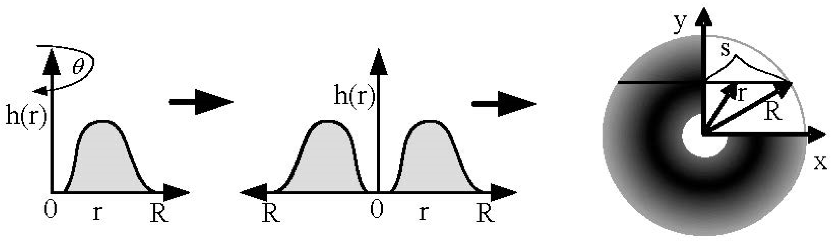
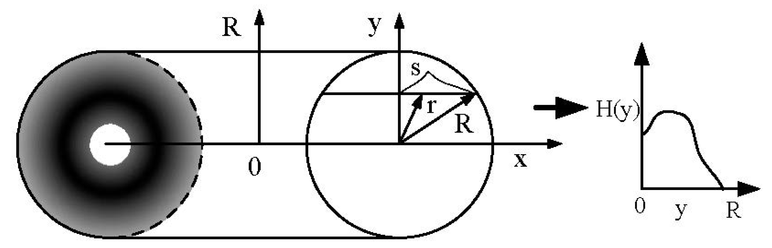
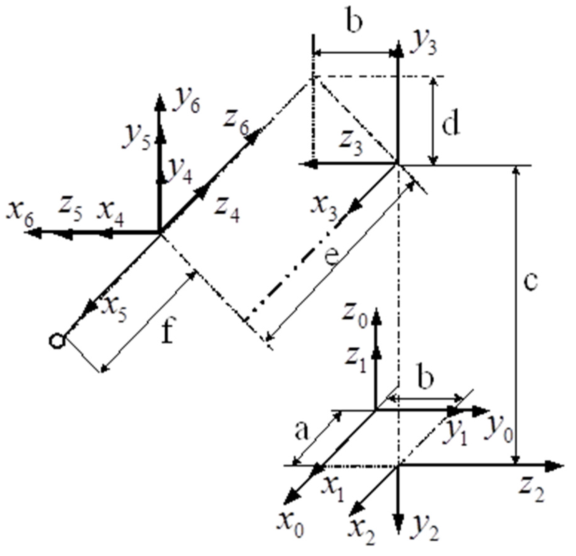
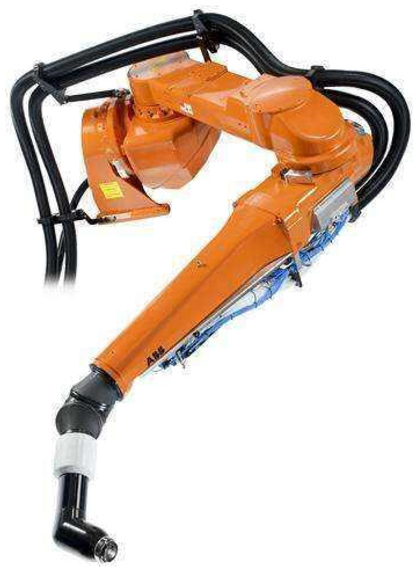
2. ESRB Spray Painting Model
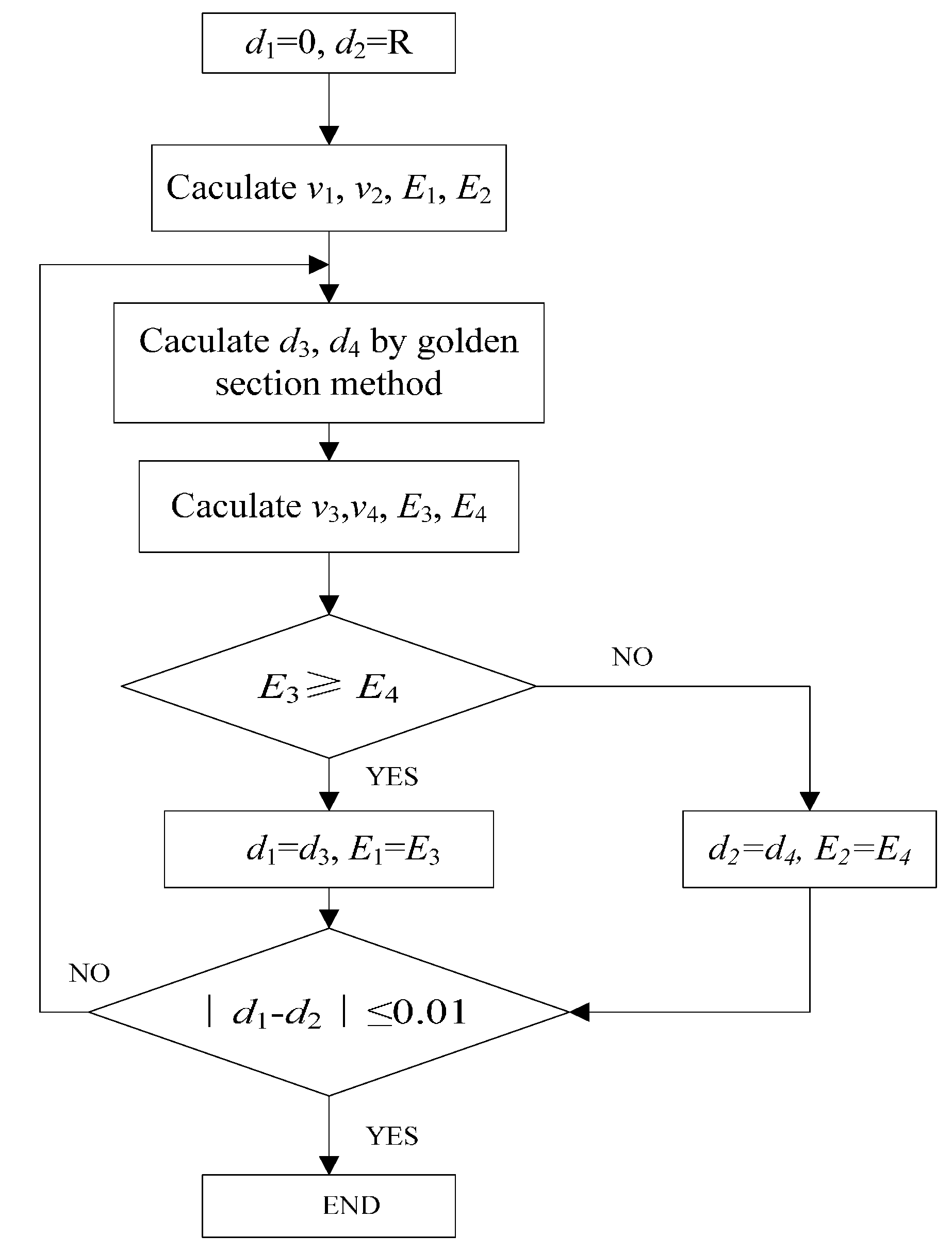
3. Spatial Path Planning Based on Cuboid Model
- 1)
- The surface is determined by the CAD (Computer Aided Design) model of the workpiece, and the surface is divided into triangular meshes. After triangulating the surface, we can express it as a mathematical expression:where Ti is the i-th triangle in the triangular facet, and M is the total number of triangular facets in the triangular mesh.M = {Ti: i = 1, …, M}
- 2)
- Calculate the normal vector of each triangular facet, and generate a number of large patches according to the topology between adjacent triangular facets. Then, suppose that the normal vector of the surface and the normal vector of the projection plane of the surface both have the maximum angle βth (only consider that the normal vectors of the two are on the same side of the surface). After determining βth, each patch of the surface can be generated. The steps of connecting the respective triangular facets into patches are as follows:
- (1)
- Specify any of the triangular facets as the initial triangular facet.
- (2)
- Find all triangular facets that are less than the spray radius from the center point of the initial triangular facet.
- (3)
- Calculate the angle between the normal vector of all triangular facets found in Step (2) and the normal vector of the original triangular facet. If the angle is smaller than βth, connect the triangular facet with the initial triangular facet.
- (4)
- Look for the triangular facets that have not been connected into patches as a new initial triangular facet, and repeat Steps (2) and (3) until all of the triangular facets are connected into patches.
- 3)
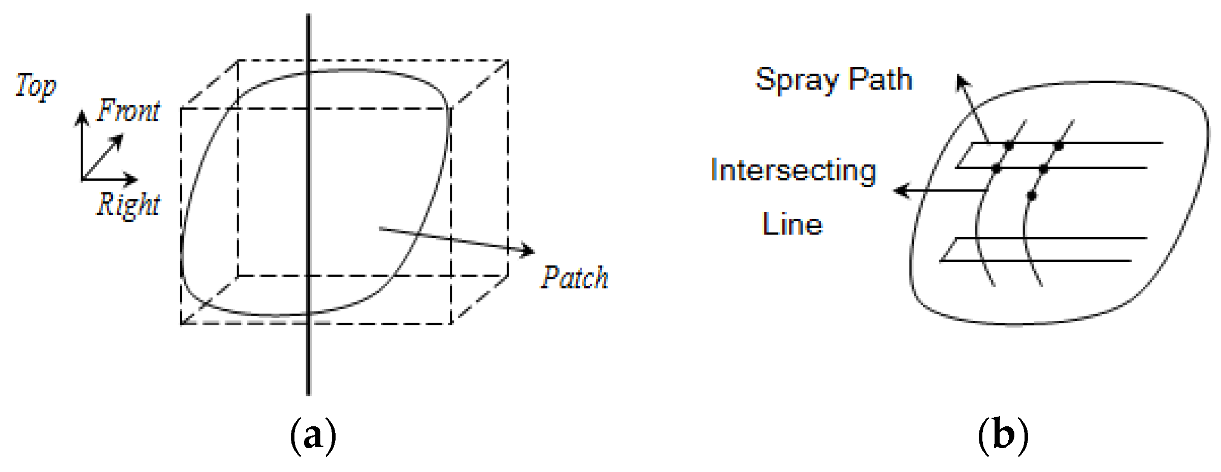
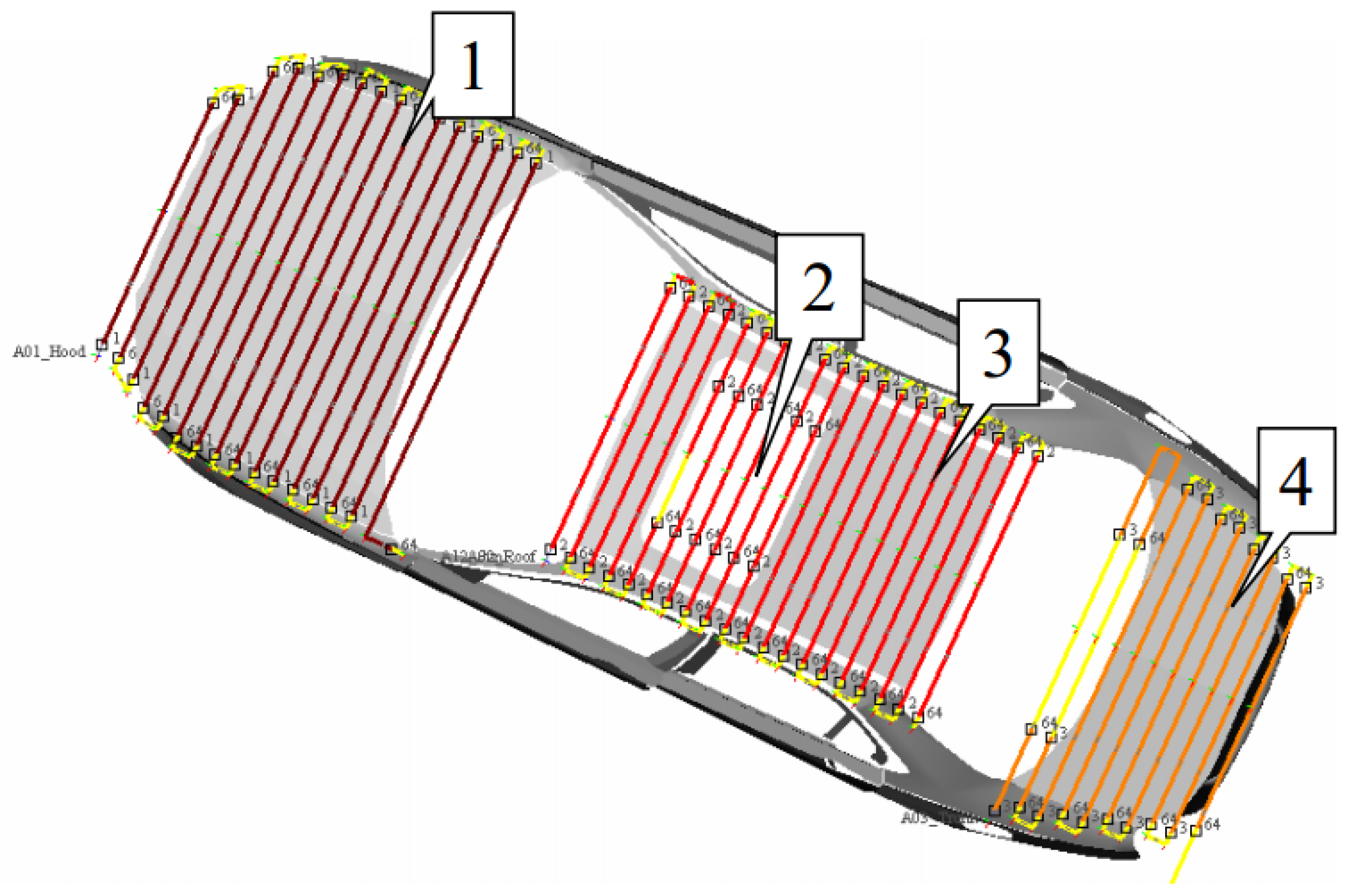
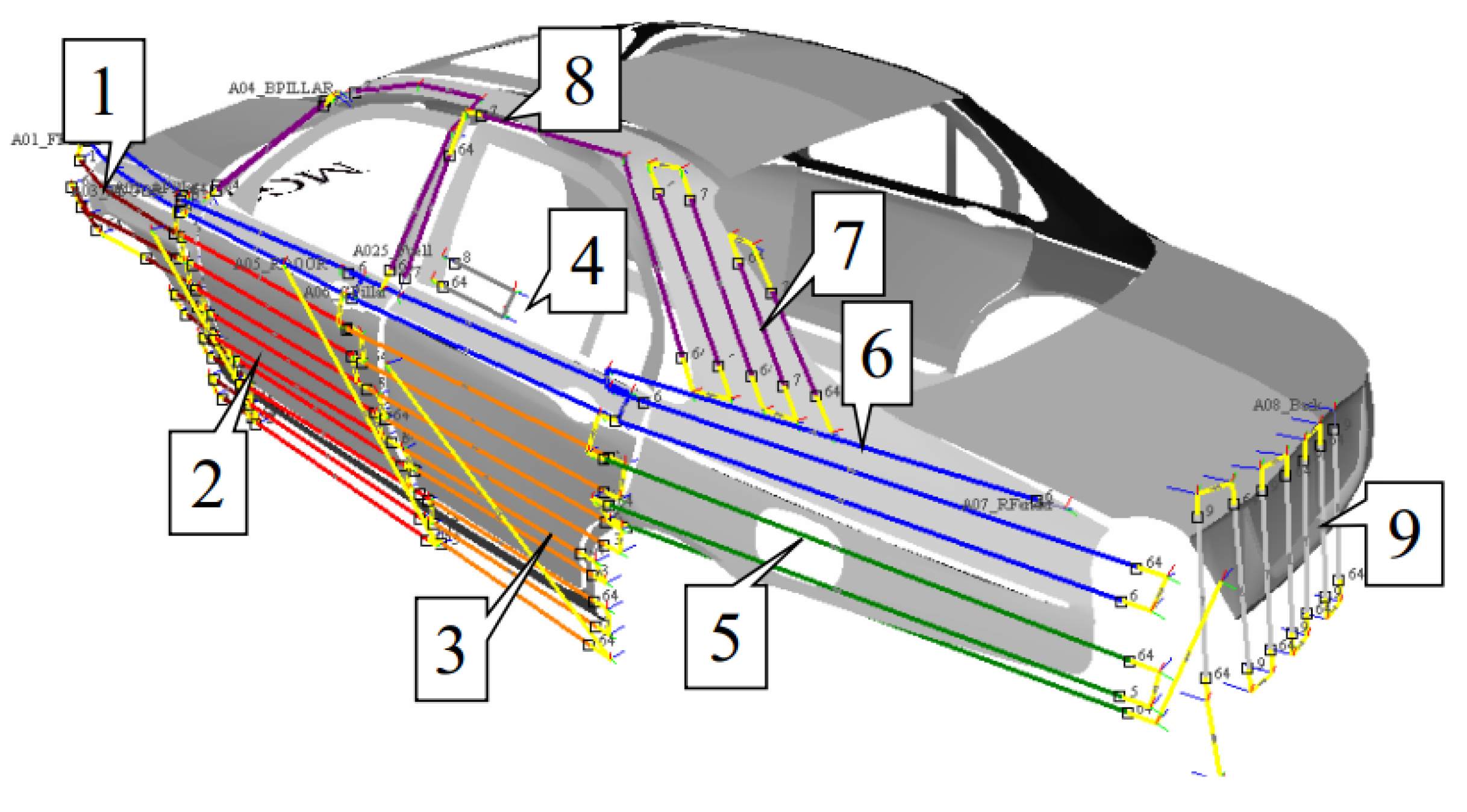
- The cuboid model is established on each patch, and the spatial path of the spray-painting robot on each patch is generated. Figure 5a shows the cuboid model established on a patch. The cuboid model is a cuboid that contains exactly the entire patch, which has two main properties: (i) its leading direction is opposite to the direction of the normal vector of the entire patch, and (ii) the area of the rectangle on each facet is as small as possible. In order to generate the spatial path of the spray-painting robot, firstly, a number of tangent planes whose distance are l (l is taken as R/2–R, R is the spray radius) are taken along the direction perpendicular to the right side of the cuboid model. Then, the intersection between the tangent plane and several segments of the curved surface can be obtained, and a series of points whose distance is d (the optimum value of the overlapping area’s width formed by two spray-painting strokes) are uniformly made on the intersecting line. Finally, these points are connected along the right side of the cuboid mode to generate the spatial path of the spray-painting robot (as shown in Figure 5b).
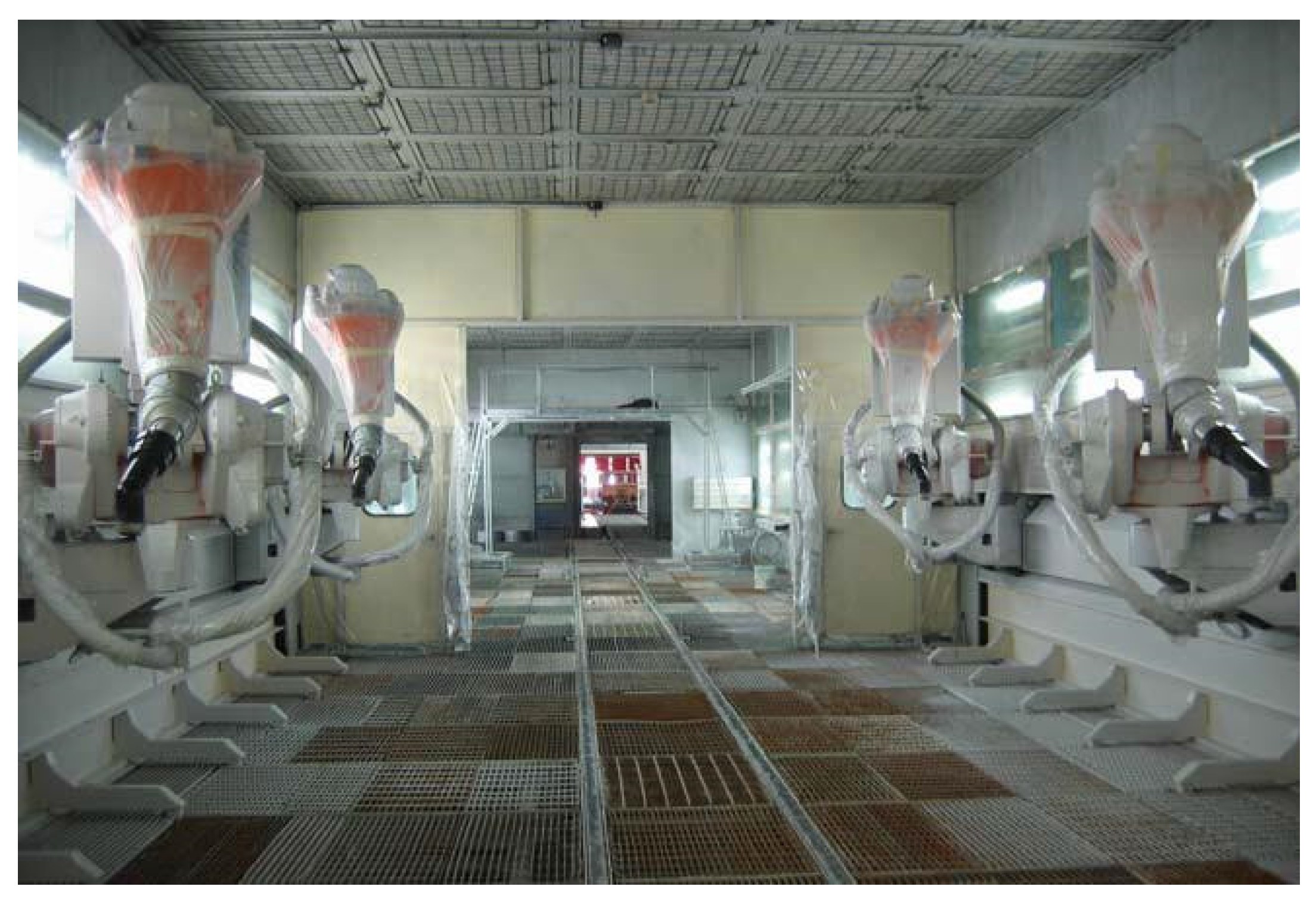
4. Electrostatic Spray-Painting Experiment
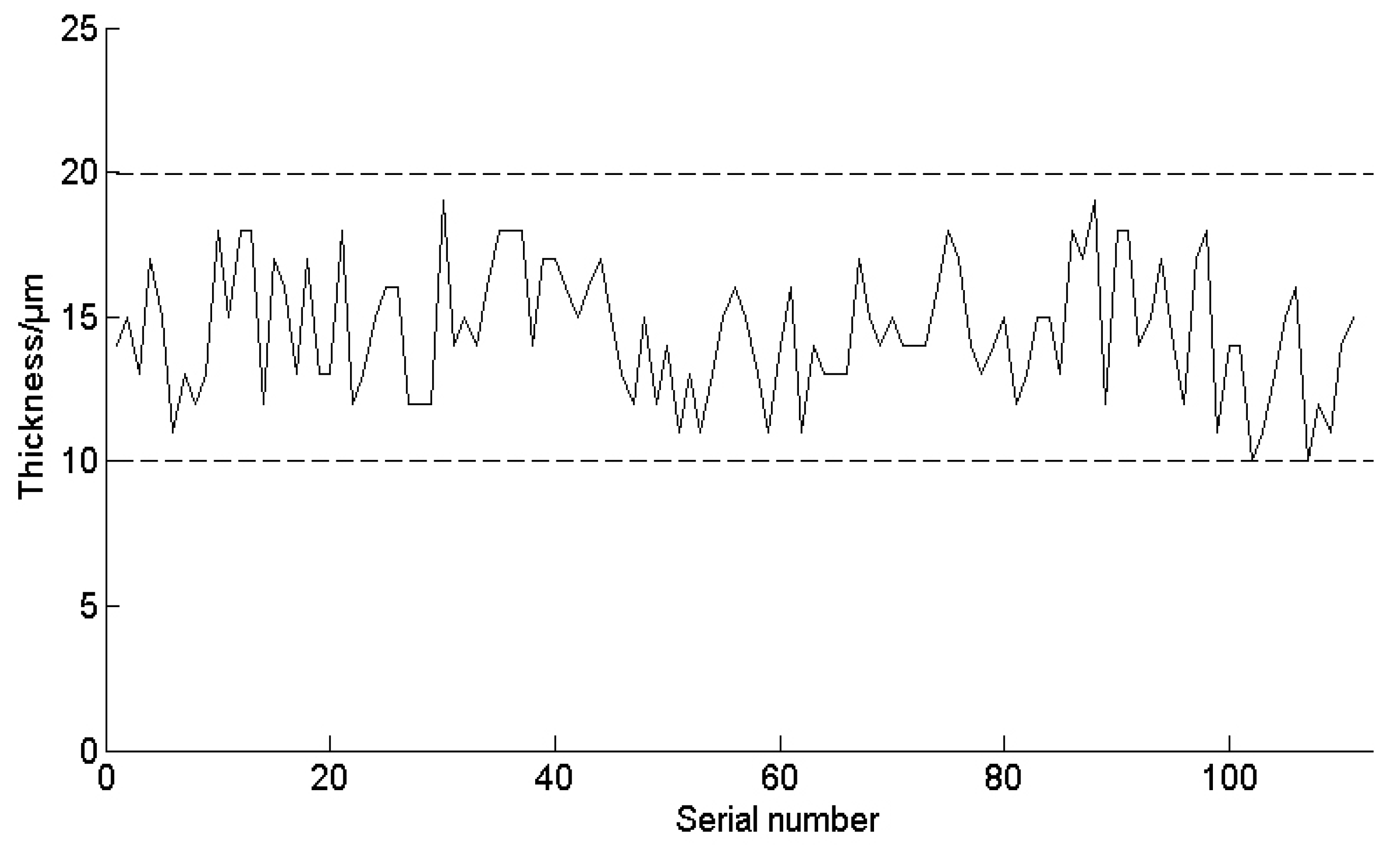
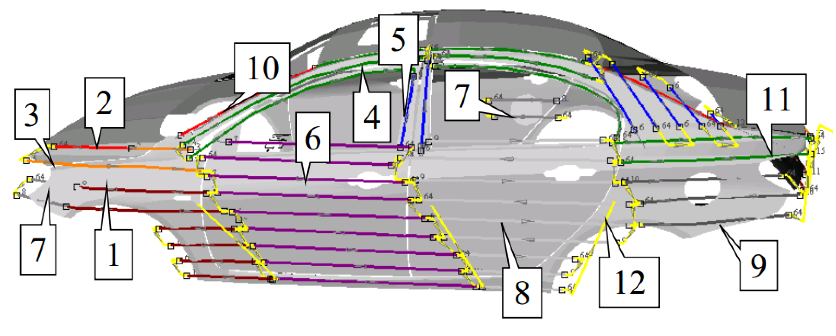
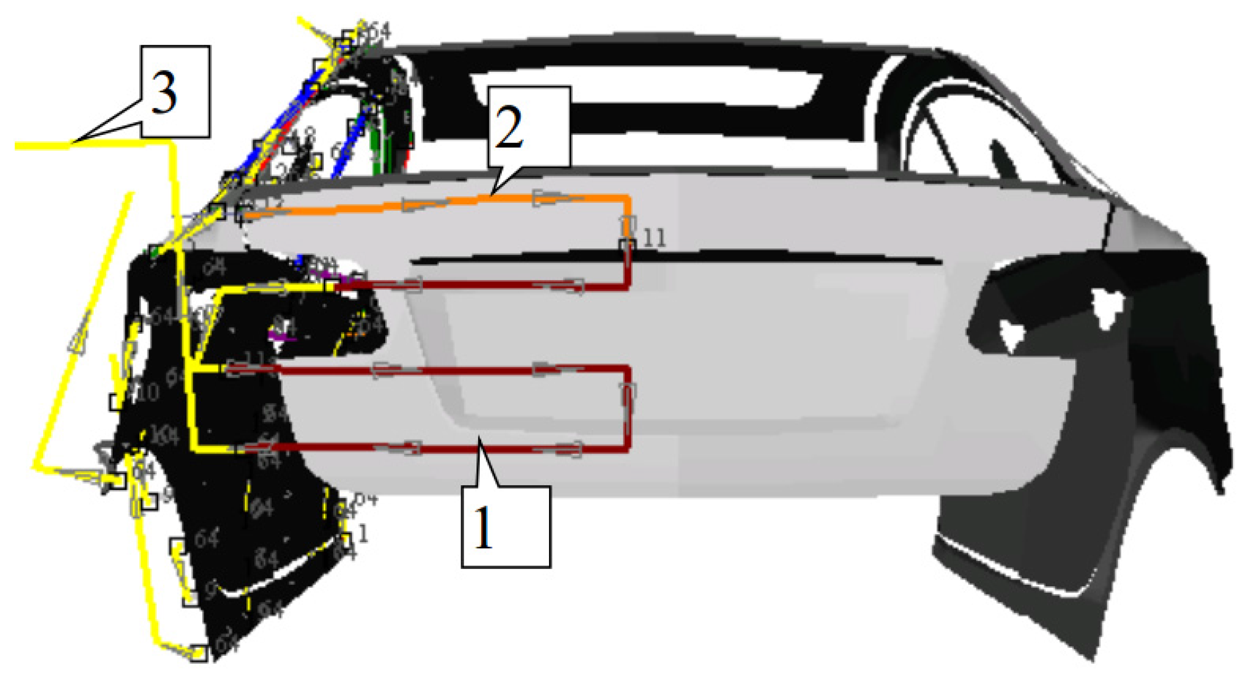
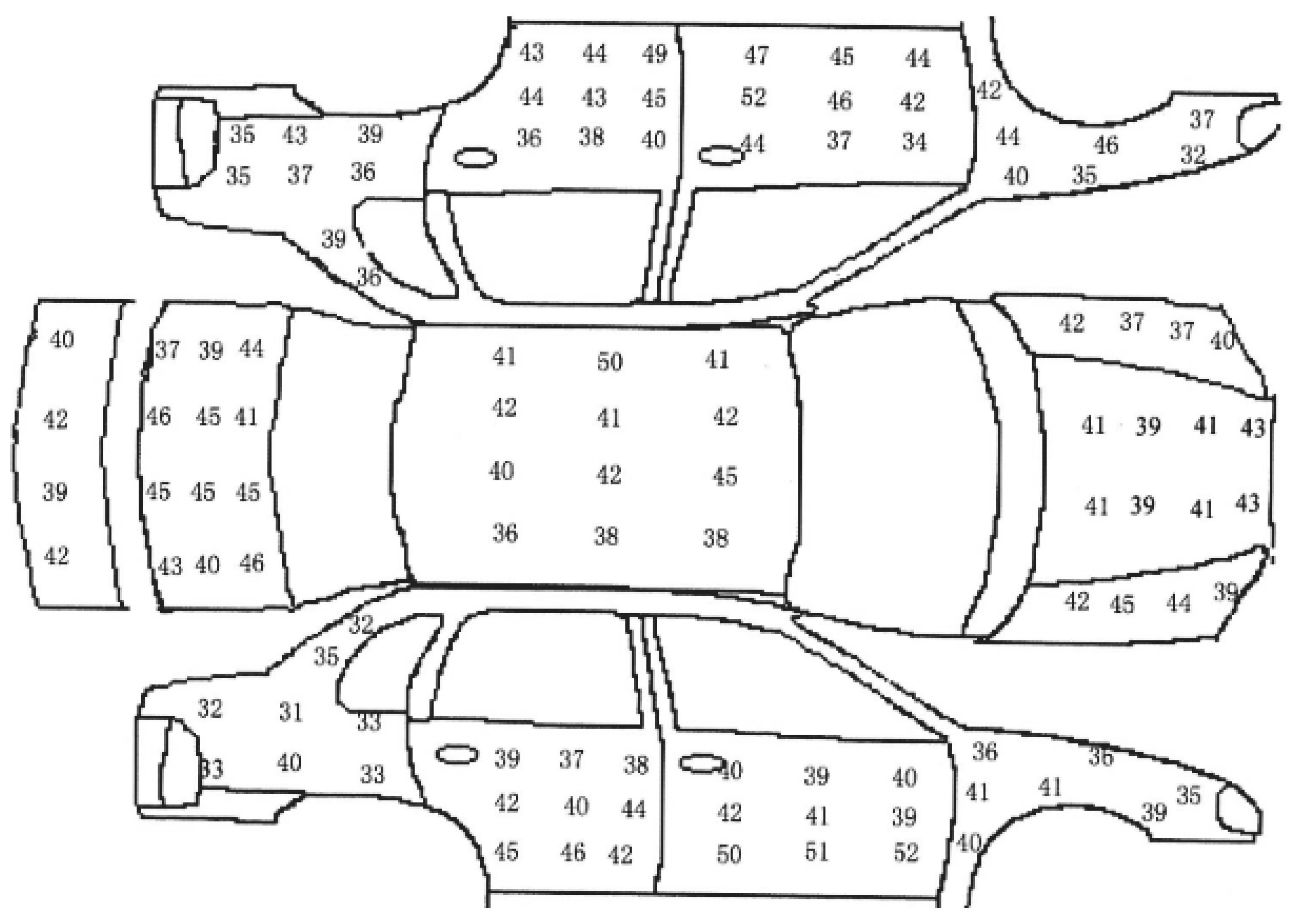
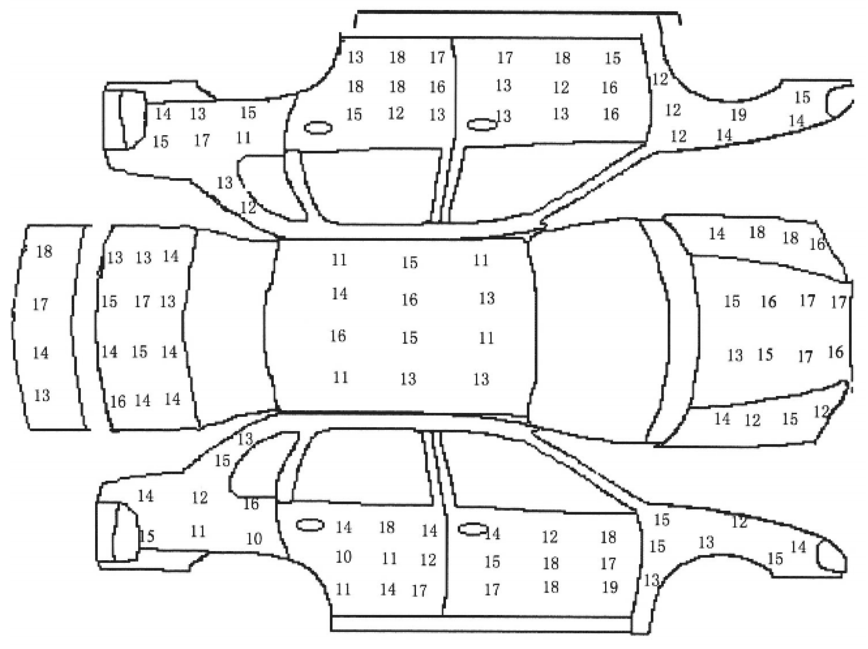
- The indicator requirements in the production process of spray-painting operation are rather high. The deviation of the maximum coating thickness set in the experiments is merely qw = ±5 × 10⁻⁶ m. For the general requirements of the spray-painting operation, the deviation of the maximum coating thickness is usually set as qw = ±10 × 10−6 m. According to this deviation threshold, the experimental result data can all meet the requirements.
- The performance of the existing spray equipment limits the consistency of the coating thickness. Due to the limitation of the memory capacity in the robot, the trajectory parameters cannot be changed unrestrictedly and continuously. Only a few trajectories can be used to approach the optimized trajectory, and the precision is not very high. When the curvature of the surface is large, the parameters of the optimized spray trajectory are greatly changed, but the parameters in the actual spray-painting operations do not change accordingly, which leads to the deviation between the results of trajectory optimization and those of the experiment.
- The curved surface of the tested automobile is too complicated. As the curved surface area of the tested automobile is large and complex and disposable spray painting is used for the whole automobile, the ESRB is in different directions when painting different parts of the body, and the effect of the gravity that affects the trajectory of the mist particles is not the same. Some parts of the surface are horizontal, some parts of the surface are tilted, and other parts of the surface are vertical. When the coating is sprayed to different surfaces, its attachment effect is also different under the influence of gravity, which is the main reason the paint thickness of the rear is small.
- Efficiency requirements of the spray painting operation are high. According to the optimization method of the spray path proposed in this paper, if we want to meet the higher spray painting requirements, more spray painting time will certainly be consumed, which will sacrifice the spray-painting efficiency. Therefore, in the actual spray painting process, the spray-painting effect and spray efficiency must reach a compromise.
5. Conclusions
Acknowledgments
Author Contributions
Conflicts of Interest
References
- Akafuah, N.; Poozesh, S.; Salaimeh, A. Evolution of the automotive body coating process—A review. Coatings 2016, 6, 24. [Google Scholar] [CrossRef]
- Akafuah, N.K.; Salazar, A.J.; Saito, K. Infrared thermography-based visualization of droplet transport in liquid sprays. Infrared Phys. Technol. 2010, 53, 218–226. [Google Scholar] [CrossRef]
- Sheng, W.H.; Xi, N.; Song, M. Automated CAD-guided robot path planning for spray painting of compound surfaces. In Proceedings of the IEEE International Conference on Intelligent Robots and Systems, Takamatsu, Japan, 30 October–5 November 2000; pp. 1918–1923. [Google Scholar]
- Freund, E.; Rokossa, D.; Roβmann, J. Process-oriented approach to an efficient off line programming of industrial robots. In Proceedings of the 24th Annual Conference of the IEEE Industrial Electronics Society, Aachen, Germany, 31 August–4 September 1998; pp. 208–213. [Google Scholar]
- Ramabhadran, R.; Antonio, J.K. Fast solution techniques for a class of optimal trajectory planning problems with applications to automated spray coating. In Proceedings of the IEEE Tansactions on Robotics and Automation, Aachen, Germany, 31 August–4 September 1998; pp. 519–530. [Google Scholar]
- Arikan, S.; Balkan, T. Process modeling, simulation and paint thickness measurement for robotic spray painting. J. Field Robot. 2000, 17, 479–494. [Google Scholar]
- Atkar, P.N.; Conner, D.C.; Greenfield, A. Hierarchical segmentation of piecewise pseudoextruded surfaces for uniform coverage. IEEE Trans. Autom. Sci. Eng. 2009, 6, 107–120. [Google Scholar] [CrossRef]
- Atkar, P.N.; Greenfield, A.; Conner, D.C. Uniform coverage of automotive surface patches. Int. J. Robotics Res. 2005, 24, 883–898. [Google Scholar] [CrossRef]
- Conner, D.C. Paint deposition modeling for trajectory planning on automotive surfaces. IEEE Trans. Autom. Sci. Eng. 2005, 2, 381–392. [Google Scholar] [CrossRef]
- Yuan, Z. Trajectory planning of Bezier curve based on improved genetic algorithm. J. Shanghai Dian Ji Univ. 2012, 15, 237–240. [Google Scholar]
- Jie, Z.; Zongyan, C.; Tiger, L.; Qingtao, L. Bézier curves of autonomous mobile robot path planning based on. J. Lanzhou Univ. 2013, 49, 249–254. [Google Scholar]
- Juhász, M.; Róth, Á. A class of generalized B-spline curves. Comput. Aided Geom. Des. 2013, 30, 85–115. [Google Scholar] [CrossRef]
- Soma, T.; Katayama, T.; Tanimoto, J. Liquid film flow on a high speed rotary bell-cup atomizer. Int. J. Multiph. Flow 2015, 70, 96–103. [Google Scholar] [CrossRef]
- Toljic, N.; Adamiak, K.; Castle, G.S.P. Three-dimensional numerical studies on the effect of the particle charge to mass ratio distribution in the electrostatic coating process. J. Electrost. 2014, 69, 189–194. [Google Scholar] [CrossRef]
- Kolakowska, E.; Smith, S.F.; Kristiansen, M. Constraint optimization model of a scheduling problem for a robotic arm in automatic systems. Robot. Autonom. Syst. 2014, 62, 267–280. [Google Scholar] [CrossRef]
- Gasparetto, A. Automatic path and trajectory planning for robotic spray painting. In Proceedings of the 7th German Conference on Robotics, Munich, German, 21–22 May 2012; pp. 211–216. [Google Scholar]
- Chen, H.P.; Sheng, W.H. Transformative industrial robot programming in surface manufacturing. In Proceedings of the IEEE International Conference on Robots and Automation, Shanghai, China, 9–13 May 2011; pp. 6059–6064. [Google Scholar]
- Chen, H.P.; Xi, N. Automated robot trajectory connection for spray forming process. J. Manuf. Sci. Eng. 2012, 134, 171–179. [Google Scholar] [CrossRef]
- Zeng, Y.; Gong, J.; Xu, N. Tool trajectory optimization of spray painting robot formany-times spray painting. Int. J. Control Autom. 2014, 7, 193–208. [Google Scholar] [CrossRef]
- Wei, C.; Yang, T.; Qiang, Z. A novel trajectory planning scheme for spray painting robot. In Proceedings of the 28th Chinese Control and Decision Conference, Yinchuan, China, 28–30 May 2016; pp. 7008–7012. [Google Scholar]
- Chen, W.; .Zhao, D. Path planning for spray painting robot of workpiece surfaces. Mathemat. Probl. Eng. 2013, 2013, 659457. [Google Scholar] [CrossRef]
- Tang, Y.; Yang, W.G.; Chen, W. Trajectory planning for spray painting robot of free-form surfaces. Appl. Mech. Mat. 2016, 543, 1309–1312. [Google Scholar] [CrossRef]
- Tang, Y.; Chen, W. Tool trajectory planning ofpainting robot and its experimental. In Proceedings of the IEEE International Conference on Mechatronics and Control, Jinzhou, China, 3–5 July 2014; pp. 872–875. [Google Scholar]
- From, P.J.; Gunnar, J.; Gravdahl, J.T. Optimal paint gun orientation in spray paint applications—Experimental results. IEEE Trans. Autom. Sci. Eng. 2013, 8, 438–442. [Google Scholar] [CrossRef]


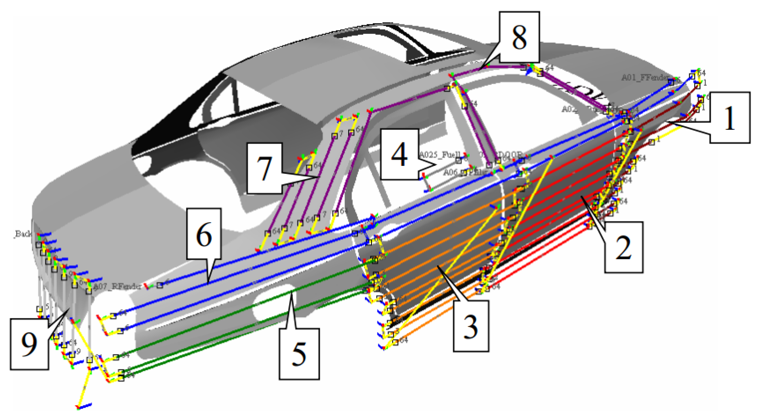
| Trajectory | Operating Parameters of Spray Trajectory on the Roof of the Tested Automobile | |||||
|---|---|---|---|---|---|---|
| No. | Colour | Del (L/min) | AM (kRPM) | SA1 (L/min) | SA2 (L/min) | HV (kV) |
| 1 |  | 290 | 40 | 250 | 180 | 60 |
| 2 |  | 240 | 40 | 250 | 180 | 60 |
| 3 |  | 300 | 40 | 250 | 220 | 60 |
| 4 |  | 200 | 40 | 250 | 180 | 60 |
| 5 |  | 200 | 40 | 250 | 180 | 60 |
| 6 |  | 280 | 40 | 250 | 180 | 60 |
| 7 |  | 0 | 40 | 280 | 180 | 60 |
| Trajectory | Operating Parameters of Spray Trajectory on the Side of the Tested Automobile | |||||
|---|---|---|---|---|---|---|
| No. | Colour | Del (L/min) | AM (kRPM) | SA1 (L/min) | SA2 (L/min) | HV (kV) |
| 1 | | 340 | 40 | 250 | 180 | 60 |
| 2 | | 100 | 40 | 250 | 180 | 60 |
| 3 | | 310 | 40 | 250 | 180 | 60 |
| 4 | | 230 | 40 | 250 | 180 | 60 |
| 5 | | 315 | 40 | 250 | 180 | 60 |
| 6 | | 285 | 40 | 250 | 180 | 60 |
| 7 |  | 370 | 40 | 250 | 180 | 60 |
| 8 |  | 285 | 40 | 250 | 180 | 60 |
| 9 |  | 310 | 40 | 250 | 180 | 60 |
| 10 | | 350 | 40 | 350 | 250 | 60 |
| 11 | | 280 | 40 | 250 | 180 | 60 |
| 12 | | 0 | 40 | 280 | 180 | 60 |
| Trajectory | Operating Parameters of Spray Trajectory on the Rear of the Tested Automobile | |||||
|---|---|---|---|---|---|---|
| No. | Colour | Del (L/min) | AM (kRPM) | SA1 (L/min) | SA2 (L/min) | HV (kV) |
| 1 | | 305 | 40 | 250 | 180 | 60 |
| 2 | | 295 | 40 | 250 | 180 | 60 |
| 3 | | 0 | 40 | 280 | 180 | 60 |
| Trajectory | Operating Parameters of Spray Trajectory on the Roof of the Tested Automobile | |||||
|---|---|---|---|---|---|---|
| No. | Colour | Del (L/min) | AM (kRPM) | SA1 (L/min) | SA2 (L/min) | HV (kV) |
| 1 | | 350 | 35 | 300 | 200 | 60 |
| 2 |  | 0 | 0 | 0 | 0 | 60 |
| 3 | | 350 | 35 | 300 | 200 | 60 |
| 4 | | 350 | 35 | 300 | 200 | 60 |
| Trajectory | Operating Parameters of Spray Trajectory on the Left and Left-Rear Parts of the Tested Automobile | |||||
|---|---|---|---|---|---|---|
| No. | Colour | Del (L/min) | AM (kRPM) | SA1 (L/min) | SA2 (L/min) | HV (kV) |
| 1 | | 350 | 35 | 300 | 200 | 60 |
| 2 | | 350 | 35 | 300 | 200 | 60 |
| 3 | | 350 | 35 | 300 | 200 | 60 |
| 4 | | 0 | 0 | 0 | 0 | 60 |
| 5 | | 350 | 35 | 300 | 200 | 60 |
| 6 | | 220 | 35 | 300 | 200 | 60 |
| 7 |  | 350 | 35 | 300 | 200 | 60 |
| 8 |  | 300 | 35 | 300 | 200 | 60 |
| 9 | | 300 | 35 | 300 | 200 | 60 |
| Trajectory | Operating Parameters of Spray Trajectory on the Right and Right-Rear Parts of the Tested Automobile | |||||
|---|---|---|---|---|---|---|
| No. | Colour | Del (L/min) | AM (kRPM) | SA1 (L/min) | SA2 (L/min) | HV (kV) |
| 1 | | 350 | 35 | 300 | 200 | 60 |
| 2 | | 350 | 35 | 300 | 200 | 60 |
| 3 | | 350 | 35 | 300 | 200 | 60 |
| 4 | | 0 | 0 | 0 | 0 | 60 |
| 5 | | 350 | 35 | 300 | 200 | 60 |
| 6 | | 220 | 35 | 300 | 200 | 60 |
| 7 | | 350 | 35 | 300 | 200 | 60 |
| 8 | | 300 | 35 | 300 | 200 | 60 |
| 9 | | 300 | 35 | 300 | 200 | 60 |
© 2017 by the authors. Licensee MDPI, Basel, Switzerland. This article is an open access article distributed under the terms and conditions of the Creative Commons Attribution (CC BY) license (http://creativecommons.org/licenses/by/4.0/).
Share and Cite
Chen, W.; Liu, H.; Tang, Y.; Liu, J. Trajectory Optimization of Electrostatic Spray Painting Robots on Curved Surface. Coatings 2017, 7, 155. https://doi.org/10.3390/coatings7100155
Chen W, Liu H, Tang Y, Liu J. Trajectory Optimization of Electrostatic Spray Painting Robots on Curved Surface. Coatings. 2017; 7(10):155. https://doi.org/10.3390/coatings7100155
Chicago/Turabian StyleChen, Wei, Hao Liu, Yang Tang, and Junjie Liu. 2017. "Trajectory Optimization of Electrostatic Spray Painting Robots on Curved Surface" Coatings 7, no. 10: 155. https://doi.org/10.3390/coatings7100155
APA StyleChen, W., Liu, H., Tang, Y., & Liu, J. (2017). Trajectory Optimization of Electrostatic Spray Painting Robots on Curved Surface. Coatings, 7(10), 155. https://doi.org/10.3390/coatings7100155