Modelling Thermal Conductivity of Porous Thermal Barrier Coatings

Abstract

Thermal conductivity of porous thermal barrier coatings was evaluated using a newly developed five-phase model. It was demonstrated that porosities distributed in coating strongly affect thermal conductivity. The decisive reason for this change in thermal conductivity can be traced back to defect morphology and its orientation, depending on the coating deposition technique and process parameters used during deposition. In this paper, the Bruggeman’s two-phase model was used as a reference, and a five-phase model was developed to evaluate the thermal conductivity of porous coatings. This approach uses microstructural details of the shape, size, orientation and volumetric fraction of defects of coatings as input parameters. The proposed model can predict thermal conductivity values better than the previous two-phase model.

1. Introduction

The progression in engineering alloys led to the design and development of the present era turbine engines [1]. The components of a turbine engine are exposed to elevated temperatures as well as to oxidative and corrosive gaseous environments [2,3,4]. These conditions lead to an early degradation of components due to high wear and tear at elevated temperatures. The motivation here is to protect the components from the excessive heat produced in the combustion chamber of the turbine engine. Heat transfer is related to one of the key thermo-physical parameter i.e., thermal conductivity [5,6].

Typically, gas turbine components such as combustor, turbine blades and vanes have a ceramic insulation coating known as a thermal barrier coating (TBC) [7,8], that lowers the heat transfer to the metallic base. Currently, in the gas turbine industry, there is a pressing need to reduce the thermal conductivity of ceramic coatings.

The structure of the TBC system consists of the ceramic top coat, intermetallic bond coat and superalloy substrate [9,10]. To date, most TBC top coats are based on Zirconia-Yttria oxides that are often produced by either plasma sprayed techniques or by electron beam physical vapour deposition [11,12]. The latter has been used mostly for aero-engines [13]. TBCs have been used to lower the heat transfer from the combustion gases to the metallic superalloy substrate [14]. It is evident that there is a reduction in heat transfer when a porous TBC is applied (approx. 100–300 °C with an internally cooled metallic base) [15,16,17]. Theories developed in this field indicate that TBCs can have additional benefits such as an increase in mean combustion temperature, reduction in heat loss to the cooling system, increase in the coefficient of thermal efficiency of the engine and enhancement in the fuel consumption rate [18,19,20,21,22,23,24,25]. Several techniques/methods are developed by researchers such as doping of elements, co-doping of elements, use of pyrochlore oxides, multilayer TBCs and some other techniques to lower thermal conductivity [26,27,28,29].

Further, the efficiency of a gas turbine engine can be increased with the selection of material combination that holds a low thermal conductivity over a specific elevated temperature range [30,31,32]. This holds true in the case of 8YSZ under prolonged heating. However, some materials/oxides may have even lower thermal conductivity compared to 8YSZ. But their use is limited due to drawbacks in material properties. Some of the issues are related to poor phase stability, lower fracture toughness and lower resistance to CMAS induced damage [33,34]. Low thermal conductivity and higher turbine inlet temperature are beneficial for higher engine efficiency. This, in turn, sets the requirement that the value of thermal conductivity should remain low for a longer interval under service conditions of high-temperature and high pressure [35]. Performance of the high-temperature TBC system depends on several parameters based on the microstructure of the coating. Such parameters can include the shape and orientation of the porosity, intrinsic properties of coatings, interfacial influences, doping elements, presence of rare earth metals, thickness of the coating layer, the number of defects present, and the process used to fabricate coating [20,36,37,38,39,40,41]. Some of the advanced coating techniques such as the solution precursor plasma spray (SPS) method provides the ability to develop a wide range of microstructures that may have more splats with a structure similar to EB-PVD. These kinds of coatings can be deposited at an ultra-fine level that will have a longer life than EB-PVD under set conditions [42,43,44].

Changes in these parameters will induce variations in thermal properties. Therefore, it is essential to design/model the desired thermal properties prior to final fabrication of actual coatings and to infer theoretically the experimental results [45,46]. The modelling of thermal conductivity is used to better understand the effects of different parameters on the matrix’s total conductivity. Indirect methods of measuring the thermal conductivity only provide the final conductivity value without providing any insights on how a lower value is achieved. The goal of this research work is to enhance the analytical modelling capability of thermal conductivity in order to better understand the effects of different size and orientation of defects and pores at macroscopic to Nano-scale level. Further modelling of thermal properties proved a quite efficient approach with respect to time and funds. Although thermal conductivity can be indirectly measured by measuring thermal diffusivity, a simple but relatively accurate approach to modelling thermal conductivity would permit a better understanding of the parameters that control the final thermal conductivity and an improved understanding of the relative influence they command on the final thermal conductivity of the coating.

To model thermal conductivity, the effect of shape, size, orientation and volumetric fraction of the defects/porosity should be considered. These considerations are present in Bruggeman’s two-phase model [47]. Therefore, in this paper, a brief introduction to Bruggeman’s two-phase is presented and the two-phase model as a reference, and then a five-phase model to predict the thermal conductivity of porous coatings is developed and applied.

2. Bruggeman Two-Phase Model for Thermal Conductivity

Thermal conductivity (k), is simply a measure of heat transfer from one surface to another through cross-sectional area A and is separated by a distance L. The thermal conductivity of free-standing materials can be evaluated by [48]

$$k=\mathsf{\alpha }·C_{\mathrm{p}}·\mathsf{\rho }$$

(1)

where ρ is the density of the free-standing material (kg/m⁻³), C_p indicates the heat capacity of the material at constant pressure (J/(kg K)), and α is the thermal diffusion rate (m²/s) [48]. Bruggeman introduced a model to predict the thermal conductivity of porous ceramic coatings [47]. He significantly improved the asymmetrical modelling capability by extending the Maxwell model to systems with random dispersions of dilute spherical particles that vary within an infinite range of values. The basis of his research was the assumption that each sphere is embedded in a continuous matrix. His model assumes that if a relatively large spherical particle is introduced into a dispersion containing much smaller particles, there will be a negligible disturbance of the field around the large sphere due to the small spheres. With this model, he showed that the limitation on a volumetric fraction of dilute dispersion can be removed (0 ≤ f ≤ 1). Bruggeman designed the model for a porous TBC system, which assumes that only one type of defect is present in a continuous matrix. Representation of such coatings can be seen in Figure 1. The Maxwell model was extended by Bruggeman as [49]

$$\frac{k-k_{\mathrm{m}}}{k+2k_{\mathrm{m}}}=f\frac{k_{\mathrm{d}}-k_{\mathrm{m}}}{k_{\mathrm{d}}+2k_{\mathrm{m}}}$$

(2)

where k is the thermal conductivity of the composite, k_m is the thermal conductivity of the matrix, k_d is the thermal conductivity of the dispersed phase and f is the volumetric fraction of the i^th phase. Further, the change in the conductivity dM i.e., k − k_m, with a change in the volume fraction f of the dispersed phase, is expressed as,

$$\frac{\mathrm{d}M}{3M}=\frac{\mathrm{d}P}{1+P}\left(\frac{k_{\mathrm{d}}-M}{k_{\mathrm{d}}+2M}\right)$$

(3)

Integrating P from 0 to f/(1 + f) and M from k_m to k leads to Bruggeman’s two-phase model, given by

$$\left(\frac{\frac{k}{k_{\mathrm{m}}}-\frac{k_{\mathrm{d}}}{k_{\mathrm{m}}}}{{\left(\frac{k}{k_{\mathrm{m}}}\right)}^{\frac{1}{3}}\left(1-\frac{k}{k_{\mathrm{d}}}\right)}\right)=(1-f)$$

(4)

In this case, it is possible to generalize the modelling to a solute dispersion of randomly oriented ellipsoids. Ellipsoids having a revolution axis corresponding to the ellipsoid axis a and with the other two equal axes i.e., b = c is the specific case of spheroids. The spheroidal shape is important because a wide range of real situations can be modelled by defining an orientation angle α, between the heat flux and the axis of revolution of the defect and by varying the ratio a/c between the two axes of the spheroid. A simple representation of a spherical shape can be seen in Figure 2. The axis a is parallel to the x-axis, b is parallel to the y-axis and c is parallel to the z-axis. There are certain shapes of the spheroid that are needed to model various types of defects. Possible shapes that can be modelled with a spheroid are shown in Figure 3. These shapes are: (i) sphere: when all axes are equal i.e., a = b = c; (ii) oblate: when axis b > a and c > a; (iii) prolate: when axis a > b and a > c.

Bruggeman’s two-phase model is simplified by the assumption that the pores/defects are non-radiating or non-conducting that means the thermal conductivity of pores/defects is assumed to be negligible, i.e., k_d = 0. This condition simplifies the model, but it should be noted that this is not a valid assumption for all temperature ranges. This assumption is only valid for temperatures where the radiative contribution to the thermal conductivity inside the pores can be neglected. Under the condition of non-radiating pores, Equation (4) reduces to,

$$\frac{k}{k\mathrm{m}}={\left(1-f\right)}^{\frac{3}{2}}$$

(5)

This equation is the special case when the pores are of spherical shape. In general, for the dispersion of an ellipsoid, the Bruggeman model is a modified version of Equation (5) and is given by [51],

$$\frac{k}{k\mathrm{m}}={\left(1-f\right)}^X$$

(6)

where X depends on certain factors such as the shape factor of the ellipsoid (F) and the orientation angle α between the heat flux and the axis of revolution. X = 3/2 for the case of spherical dispersions in a continuous matrix. The value of X can be described by [51],

$$X=\frac{1-{\cos }^2\mathsf{\alpha }}{1-F}+\frac{{\cos }^2\mathsf{\alpha }}{2F}$$

(7)

The shape factor F is an important parameter to define the value of X. It is necessary to understand the relation between the ratio of axes and the shape factor F. Corresponding to the value of a/c, the shape factor F can be obtained from the plot presented in Figure 4.

For the case of sphere-shaped defects, that is when the major and minor axis are equal (a = c), the shape factor is F = 1/3, corresponding to the axes ratio a/c = 1. When the axis a is smaller than axes b and c (c > a), the spheroid is stretched horizontally to obtain the shape of an oblate spheroid. The shape factor F for oblate (lamellas) lies between 0 and 1/3. There is an exception when the lamellae are oriented normal to the heat flux, in which case X is equal to 1. A prolate shape spheroid is obtained when pores are stretched in the vertical direction and there is a very little area in the horizontal direction. The shape factor F for prolate pores lies between 1/3 to 1/2. The value of X can also be modelled using a cylindrical shape as well. For a cylinder, the X value depends on the orientation of the major axis a. The values depend on whether the ‘a’ axis is parallel (X = 1), randomly oriented (X = 1.66) and/or perpendicular (X = 2). Figure 5 shows the ratio k/k_m as a function of the volumetric fraction of porosity at different orientations with respect to the heat flux given by the Bruggeman model in Equation (6).

3. Extension of Two-Phase Bruggeman Model to Higher Porosity Levels

In the previous section, the details regarding the Bruggeman’s two-phase model based on materials containing only one single type of defect was presented. The assumption of a material having only one type of defect is only valid for very few kinds of coatings. In reality, the TBC system is composed of a mixture of several different types of defects [36,37,51,52]. Therefore, for more realistic modelling of coatings, it becomes essential to consider several different kinds of defects that can be present in real coating’s microstructure. The models used for the evaluation of the distribution of pores can be classified as symmetrical or asymmetrical. This classification is based on the schematization of pores, either by the dispersion of the unique grains into the continuous matrix or by the symmetrical distribution of pores in the whole matrix. The modelling of several types of defects can be achieved by superimposing the contributions of different porosity types on the overall thermal conductivity. Several analytical models based on porosity have been developed and details of these are published [37,38,48,49,53,54,55,56,57]. The hybrid combination of asymmetrical and symmetrical models could predict the thermal conductivity to a higher accuracy [58]. Of these models, the Bruggeman asymmetrical model provides a better estimation of a coating’s thermal conductivity [48].

To extend the approach of coatings containing one type of defect/pore type to coatings with several types of defects/pores, an iterative approach can be used. The Bruggeman two-phase model consists of a binary mixture of dense material and spherical pores. The extension of the two-phase model to a three-phase model by using an iterative approach is presented herein.

The iterative approach works in two steps. First, the type 1 porosity is added to the continuous matrix so that the average thermal conductivity of the binary mixture of matrix and defect can be obtained. Then, for the second step, the binary mixture is considered as a continuous matrix, and subsequently, a type 2 porosity is added to the mixture. This addition of a type 2 defect at the second step will superimpose the effect of two defects on the thermal conductivity of the matrix. Consider that f₁ and f₂ are the final percentages of type 1 and type 2 porosity, respectively, then the total porosity of the coating is given by f = f₁ + f₂. There can be two ways of adding the two defects in the continuous matrix. Consider if we add a type 1 porosity first into the continuous matrix and then add a type 2 porosity, this will lead to an expression given by,

$$\left\{\mathsf{\Phi }\left[\frac{f_2}{1-f_1}\right]\mathsf{\Psi }\left(f_1\right)\right\}$$

(8)

where Ψ(f) and Φ(f) are functions describing the effect of defects on the thermal conductivity of the coating. Now consider if we first add a type 2 porosity in the continuous matrix and then type 1, this will generate an expression given by,

$$\left\{\mathsf{\Psi }\left[\frac{f_1}{1-f_2}\right]\mathsf{\Phi }\left(f_2\right)\right\}$$

(9)

The model for higher porosity content is formulated by averaging the multiple values of the constituents that directly make up the composite material. Therefore, when the two possible cases are averaged, the thermal conductivity of the three-phase mixture [50,51] is given as,

$$k=\frac{k_0}{2}\left\{\mathsf{\Psi }\left[\frac{f_1}{\left(1-f_2\right)}\right]\mathsf{\Phi }\left(f_2\right)+\mathsf{\Phi }\left[\frac{f_2}{\left(1-f_1\right)}\right]\mathsf{\Psi }\left(f_1\right)\right\}$$

(10)

This process is also known as an averaging technique. Equation (10) is symmetrical with respect to the product of Ψ(f) and Φ(f) in order to satisfy the commutative properties of the dilution process. This property helps to produce a unique solution. This process of averaging all the possible ways in which different types of defects can be added will provide the formula for n defects under consideration.

4. Proposed Five-Phase Model for Thermal Conductivity

The high-temperature performance of TBCs is greatly influenced by microstructural features [59,60,61]. Assessing the influences of microstructural changes will help to obtain the desired coating properties. Analysis of the coating microstructure can be performed experimentally or analytically. The cost-effectiveness of an analytical approach outweighs the use of the experimental method in the design of a coating. The performance of the TBC is related to porosity; hence it became essential to model the thermal properties according to the porosity distribution.

Analytical models use detailed information from previously available information to meet the complex design needs of thermal barrier coatings [62]. The thermal conductivity is strongly influenced by entrapped air or liquid in the pores. In general, coating defects can be classified as open porosity, horizontal crack, microcrack, splat interfaces, vertical crack or randomly oriented pore and crack [63]. Figure 6 provides an overview of the various types of defects.

The distribution of porosity in the analytical model can be presented precisely; however, certain conditions need to be considered. For example, the model must contain adequate microstructural details to represent the properties of the sample [64]. Even small details regarding the microstructural features of the coating must be included so that the actual properties can be modelled precisely. Some basic assumptions used in this work for effective modelling of the porous ceramic coatings are as follows: (a) The pores are assumed to be non-conducting or non-radiating i.e., the thermal conductivity of the pores is assumed to be negligible (k_d = 0) (for certain temperature limits under consideration); (b) there is an inverse proportionality between porosity content and thermal conductivity of the porous composite; (c) heat transfer is along the thickness of the coating only (or perpendicular to the bond coat–substrate interface). No lateral heat transfer is assumed; (d) the effect of connected pores is neglected.

The goal of this work is to enhance the analytical modelling capability to better predict the overall thermal conductivity of a ceramic coating by using a five-phase mixture. In the proposed five-phase model presented here, four different types of the pores/defects are assumed to be embedded into the continuous matrix. The effect of each type of defect is represented by a function. Φ(f) represents the effect of open randomly oriented pores on thermal conductivity. Ψ(f) represents the effect of pores with a revolution axis oriented parallel to heat flux. Θ(f) represents the effect of non-flat spheroidal porosities. Γ(f) represents the effect of pores with a revolution axis oriented perpendicular to heat flux.

In this work, the total porosity f is the sum of the volumetric fraction of all the different types of defects present in the coating and is given by f = f₁ + f₂ + f₃ + f₄. The effect of any type of defect is described by the functions Φ, Ψ, Θ and Γ and the values of these functions are given by the Equation (11) as

$$\mathsf{\Psi }\left(f\right)={\left(1-f\right)}^X$$

(11)

The values of the volumetric function f of different porosity types are obtained from existing works [51,52,65,66], as well as from image analysis using Image J. The addition of four different types of porosities simultaneously into the continuous matrix is carried out using the iterative approach. This gives the formula of a five-phase composite material that consists of twenty-four equations. For better understanding, the formula for the five-phase model is divided into four parts. This process does not affect the formula in any manner as all four parts simply sum. The five-phase model can be expressed as

$$k=\frac{k_0}{24}\left(A+B+C+D\right)$$

(12)

where k is the overall thermal conductivity of the porous coating, k₀ is the thermal conductivity of dense coating or matrix, and A, B, C and D provide simplification of the formula. The formula averages all the possible conditions in which the four different types of defects can be added in different orders. The expressions for A, B, C and D are given as follows:

$$\begin{array}{l}A=\left\{\{\left(\frac{\mathsf{\Psi }(f_1)}{1-\left(f_2+f_3+f_4\right)}\right)\ast \left(\frac{\mathsf{\Phi }(f_2)}{1-(f_3+f_4)}\right)\ast \left(\frac{\mathsf{\Theta }(f_3)}{1-f_4}\right)\ast (\mathsf{\Gamma }(f_4))\right\}+\\ \{\left(\frac{\mathsf{\Psi }(f_1)}{1-\left(f_2+f_3+f_4\right)}\right)\ast \left(\frac{\mathsf{\Phi }(f_2)}{1-(f_3+f_4)}\right)\ast \left(\frac{\mathsf{\Gamma }(f_4)}{1-f_3}\right)\ast (\mathsf{\Theta }(f_3))\}+\\ \{\left(\frac{\mathsf{\Psi }(f_1)}{1-\left(f_2+f_3+f_4\right)}\right)\ast \left(\frac{\mathsf{\Theta }(f_3)}{1-(f_2+f_4)}\right)\ast \left(\frac{\mathsf{\Phi }(f_2)}{1-f_4}\right)\ast (\mathsf{\Gamma }(f_4))\}+\\ \{\left(\frac{\mathsf{\Psi }(f_1)}{1-\left(f_2+f_3+f_4\right)}\right)\ast \left(\frac{\mathsf{\Theta }(f_3)}{1-(f_2+f_4)}\right)\ast \left(\frac{\mathsf{\Gamma }(f_4)}{1-f_2}\right)\ast (\mathsf{\Phi }(f_2))\}+\\ \{\left(\frac{\mathsf{\Psi }(f_1)}{1-\left(f_2+f_3+f_4\right)}\right)\ast \left(\frac{\mathsf{\Gamma }(f_4)}{1-(f_2+f_3)}\right)\ast \left(\frac{\mathsf{\Phi }(f_2)}{1-f_3}\right)\ast (\mathsf{\Theta }(f_3))\}+\\ \{\left(\frac{\mathsf{\Psi }(f_1)}{1-\left(f_2+f_3+f_4\right)}\right)\ast \left(\frac{\mathsf{\Gamma }(f_4)}{1-(f_2+f_3)}\right)\ast \left(\frac{\mathsf{\Theta }(f_3)}{1-f_2}\right)\ast (\mathsf{\Phi }(f_2))\}\end{array}$$

(13)

$$\begin{array}{l}B=\left\{\{\left(\frac{\mathsf{\Phi }(f_2)}{1-\left(f_1+f_3+f_4\right)}\right)\ast \left(\frac{\mathsf{\Psi }(f_1)}{1-(f_3+f_4)}\right)\ast \left(\frac{\mathsf{\Theta }(f_3)}{1-f_4}\right)\ast (\mathsf{\Gamma }(f_4))\right\}+\\ \{\left(\frac{\mathsf{\Phi }(f_2)}{1-\left(f_1+f_3+f_4\right)}\right)\ast \left(\frac{\mathsf{\Psi }(f_1)}{1-(f_3+f_4)}\right)\ast \left(\frac{\mathsf{\Gamma }(f_4)}{1-f_3}\right)\ast (\mathsf{\Theta }(f_3))\}+\\ \{\left(\frac{\mathsf{\Phi }(f_2)}{1-\left(f_1+f_3+f_4\right)}\right)\ast \left(\frac{\mathsf{\Theta }(f_3)}{1-(f_1+f_4)}\right)\ast \left(\frac{\mathsf{\Psi }(f_1)}{1-f_4}\right)\ast (\mathsf{\Gamma }(f_4))\}+\\ \{\left(\frac{\mathsf{\Phi }(f_2)}{1-\left(f_1+f_3+f_4\right)}\right)\ast \left(\frac{\mathsf{\Theta }(f_3)}{1-(f_1+f_4)}\right)\ast \left(\frac{\mathsf{\Gamma }(f_4)}{1-f_1}\right)\ast (\mathsf{\Psi }(f_1))\}+\\ \{\left(\frac{\mathsf{\Phi }(f_2)}{1-\left(f_1+f_3+f_4\right)}\right)\ast \left(\frac{\mathsf{\Gamma }(f_4)}{1-(f_1+f_3)}\right)\ast \left(\frac{\mathsf{\Psi }(f_1)}{1-f_3}\right)\ast (\mathsf{\Theta }(f_3))\}+\\ \{\left(\frac{\mathsf{\Phi }(f_2)}{1-\left(f_1+f_3+f_4\right)}\right)\ast \left(\frac{\mathsf{\Gamma }(f_4)}{1-(f_1+f_3)}\right)\ast \left(\frac{\mathsf{\Theta }(f_3)}{1-f_1}\right)\ast (\mathsf{\Psi }(f_1))\}\end{array}$$

(14)

$$\begin{array}{l}C=\left\{\{\left(\frac{\mathsf{\Theta }(f_3)}{1-\left(f_1+f_2+f_4\right)}\right)\ast \left(\frac{\mathsf{\Psi }(f_1)}{1-(f_2+f_4)}\right)\ast \left(\frac{\mathsf{\Phi }(f_2)}{1-f_4}\right)\ast (\mathsf{\Gamma }(f_4))\right\}+\\ \{\left(\frac{\mathsf{\Theta }(f_3)}{1-\left(f_1+f_2+f_4\right)}\right)\ast \left(\frac{\mathsf{\Psi }(f_1)}{1-(f_2+f_4)}\right)\ast \left(\frac{\mathsf{\Gamma }(f_4)}{1-f_3}\right)\ast (\mathsf{\Phi }(f_2))\}+\\ \{\left(\frac{\mathsf{\Theta }(f_3)}{1-\left(f_1+f_2+f_4\right)}\right)\ast \left(\frac{\mathsf{\Phi }(f_2)}{1-(f_1+f_4)}\right)\ast \left(\frac{\mathsf{\Psi }(f_1)}{1-f_4}\right)\ast (\mathsf{\Gamma }(f_4))\}+\\ \{\left(\frac{\mathsf{\Theta }(f_3)}{1-\left(f_1+f_2+f_4\right)}\right)\ast \left(\frac{\mathsf{\Phi }(f_2)}{1-(f_1+f_4)}\right)\ast \left(\frac{\mathsf{\Gamma }(f_4)}{1-f_1}\right)\ast (\mathsf{\Psi }(f_1))\}+\\ \{\left(\frac{\mathsf{\Theta }(f_3)}{1-\left(f_1+f_2+f_4\right)}\right)\ast \left(\frac{\mathsf{\Gamma }(f_4)}{1-(f_1+f_2)}\right)\ast \left(\frac{\mathsf{\Psi }(f_1)}{1-f_2}\right)\ast (\mathsf{\Phi }(f_2))\}+\\ \{\left(\frac{\mathsf{\Theta }(f_3)}{1-\left(f_1+f_2+f_4\right)}\right)\ast \left(\frac{\mathsf{\Gamma }(f_4)}{1-(f_1+f_2)}\right)\ast \left(\frac{\mathsf{\Phi }(f_2)}{1-f_1}\right)\ast (\mathsf{\Psi }(f_1))\}\end{array}$$

(15)

$$\begin{array}{l}D=\left\{\{\left(\frac{\mathsf{\Gamma }(f_4)}{1-\left(f_1+f_3+f_2\right)}\right)\ast \left(\frac{\mathsf{\Psi }(f_1)}{1-(f_3+f_2)}\right)\ast \left(\frac{\mathsf{\Theta }(f_3)}{1-f_2}\right)\ast (\mathsf{\Phi }(f_2))\right\}+\\ \{\left(\frac{\mathsf{\Gamma }(f_4)}{1-\left(f_1+f_3+f_2\right)}\right)\ast \left(\frac{\mathsf{\Psi }(f_1)}{1-(f_3+f_2)}\right)\ast \left(\frac{\mathsf{\Phi }(f_2)}{1-f_3}\right)\ast (\mathsf{\Theta }(f_3))\}+\\ \{\left(\frac{\mathsf{\Gamma }(f_4)}{1-\left(f_1+f_3+f_2\right)}\right)\ast \left(\frac{\mathsf{\Theta }(f_3)}{1-(f_1+f_2)}\right)\ast \left(\frac{\mathsf{\Psi }(f_1)}{1-f_2}\right)\ast (\mathsf{\Phi }(f_2))\}+\\ \{\left(\frac{\mathsf{\Gamma }(f_{14})}{1-\left(f_1+f_3+f_2\right)}\right)\ast \left(\frac{\mathsf{\Theta }(f_3)}{1-(f_1+f_2)}\right)\ast \left(\frac{\mathsf{\Phi }(f_2)}{1-f_1}\right)\ast (\mathsf{\Psi }(f_1))\}+\\ \{\left(\frac{\mathsf{\Gamma }(f_4)}{1-\left(f_1+f_3+f_2\right)}\right)\ast \left(\frac{\mathsf{\Phi }(f_2)}{1-(f_1+f_3)}\right)\ast \left(\frac{\mathsf{\Psi }(f_1)}{1-f_3}\right)\ast (\mathsf{\Theta }(f_3))\}+\\ \{\left(\frac{\mathsf{\Gamma }(f_4)}{1-\left(f_1+f_3+f_2\right)}\right)\ast \left(\frac{\mathsf{\Phi }(f_2)}{1-(f_1+f_3)}\right)\ast \left(\frac{\mathsf{\Theta }(f_3)}{1-f_1}\right)\ast (\mathsf{\Psi }(f_1))\}\end{array}$$

(16)

By averaging all the possibilities of the accumulation of defects, the five-phase formula is constructed. Each type of defect has its own shape factor F and X-factor. The systematic approach of obtaining the thermal conductivity of the coating can be understood using the flowchart in Figure 7. The calculations for shape factor F and X values are performed in the next section.

4.1. Calculation of the Values of Variables for the Five-Phase Model

It is known that the orientation of the pores and cracks can impact the overall thermal conductivity [36,67,68]. A small deviation in the axes of the pores will result in a different value for the thermal conductivity, even for materials with the same composition [69]. As discussed in the preceding section, the X values vary according to the shape under consideration.

The first step for the model is to obtain the length, height and orientation angle α of the defects from the SEM images using Image J software. SEM images reflecting coating’s structure and features have been included in Appendix A. Image analysis provides details regarding the length of the axis in horizontal and vertical directions. After obtaining the axis ratio a/c, the shape factor F is obtained by tracing back on the curve presented in Figure 4. The F values vary according to the different kinds of shapes and orientation of defects.

The value of shape factor F for horizontal types of defects or lamellae lies within the range of 0–1/3. Vertical types of defects or cylindrical defects have a shape factor F in the range of 1/3–1/2. Tiny voids are often represented by a sphere, but in most cases, these pores get elongated during thermal cycling under the influence of thermal stress and mismatch between the thermal expansion coefficient of different materials [70]. It is apparent from the work of Hasselman that the pores that are horizontal or splat-like (perpendicular to the direction of heat flow) are more beneficial in reducing thermal conductivity compared to the pores that are aligned parallel to the direction of heat flux (i.e., vertical pores) [68]. This explains the lower thermal conductivity of APS coatings as compared to EB-PVD TBCs. APS coatings have a more splat structure (lamellae porosity), which lowers the heat transfer compared to EB-PVD coatings [56].

After obtaining the values for specific shape factors and orientations, X values are calculated for the different pores using Equation (7). The values of X-factor are calculated at various angles, such as 0°, 30°, 45°, 60° and 90°. The difference caused by changing the orientation of an axis can be seen in the figures below. Figure 8 and Figure 9 represent the relation between the values of X corresponding to the values of F at an orientation angle α of 0 degrees. Changing the angle of the axis of revolution corresponding to heat flux from 0° to 30° affects the values of F and ultimately the values of X. Figure 10 represents the changes in the values of X for the variation in angle α from 0° to 30°. The change in the curvature of the graph provides evidence to support the dependence of X values on the shape factor F. 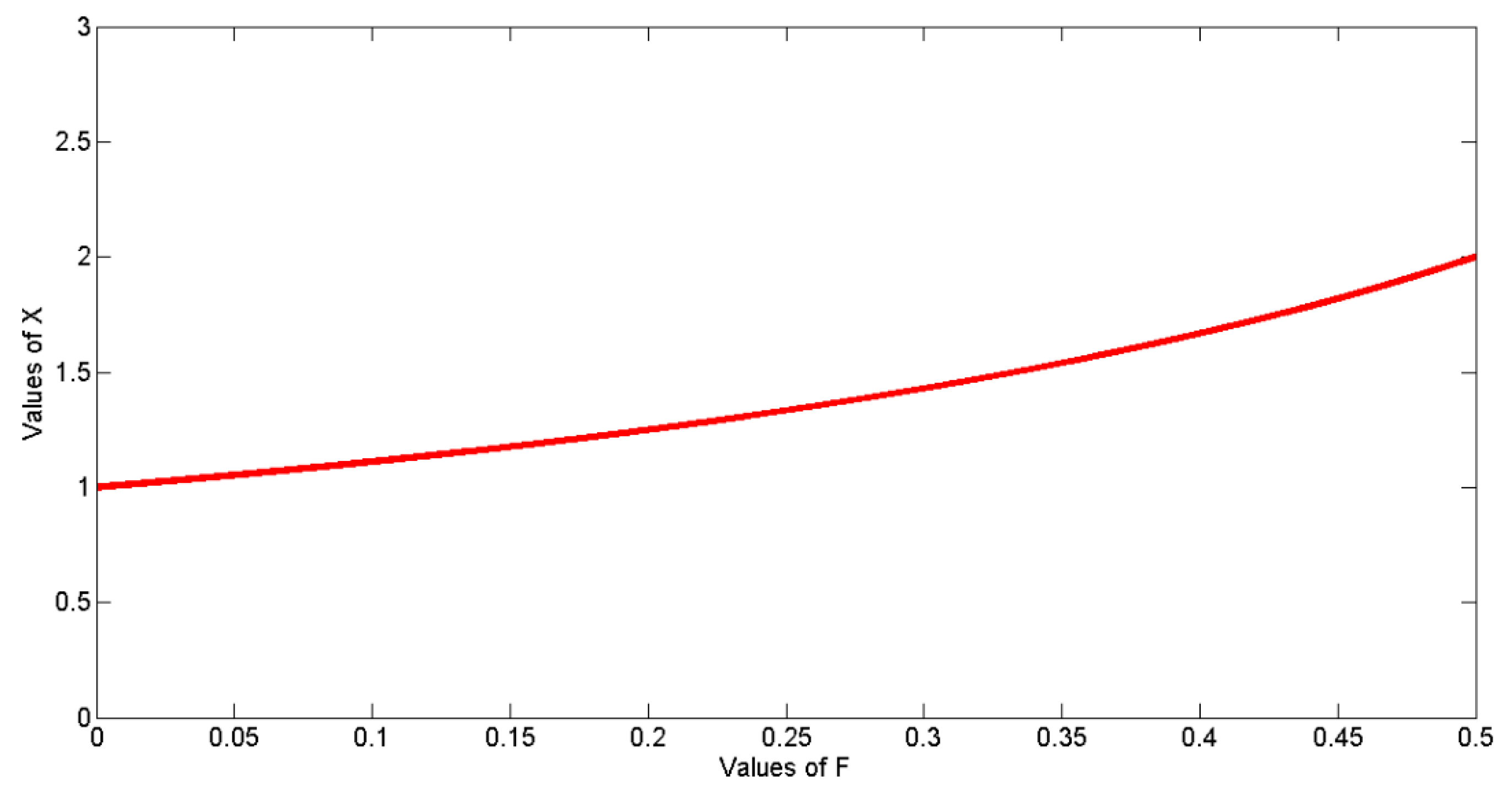Figure 11 represents the relationship between X and F for an angle α = 45°. Figure 12 illustrates the results obtained from the calculation of the X-factor corresponding to F at an angle of 60° between the axis of revolution of the spheroid and heat flux.

It can be seen from the figures presented in this section that there is a variation in the values of X with increasing angle α. When the axis of revolution is directly perpendicular to the heat flux, the value of X increases with an increase of shape factor F. This can be clearly seen in Figure 13, where the starting value of X is lowest and tends to increase with increasing value of F. The results obtained from these graphs are used in the proposed five-phase model for porous coatings to calculate the thermal conductivity of different materials.

4.2. Obtaining Values of Functions in the Five-Phase Model

For the computation of thermal conductivity using the Equation (12), the values of the functions Φ, Ψ, Θ and Γ are defined and evaluated using Equation (11) and the respective equations can be obtained from the

Table 1. The equations for different X values due to different F and α.

Function	Representation in Terms of X
Open randomly oriented–Φ(f)	${\left(1-f\right)}^{X_1}$
Revolution axis oriented parallel to heat flux–Ψ(f)	${\left(1-f\right)}^{X_2}$
Non-flat spheroids–Θ(f)	${\left(1-f\right)}^{X_3}$
Revolution axis oriented perpendicular to heat flux–Γ(f)	${\left(1-f\right)}^{X_4}$

.

When the length of the axes (a, b and c) are close to each other, then the ratio of axes is equal to one and the shape factor is F = 0.3333. At any given angle, the value of X is always equal to 1.5. This shows that the shape being modelled is a sphere, as there is no change in the value of X with a change in the orientation of the pore (see

Table 2. The X values obtained for the shape factor for F = 1/3 at different angles.

Angle α	X Values
At 0°	1.5
At 30°	1.5
At 45°	1.5
At 60°	1.5
At 90°	1.5

). In actual coatings, there are very few voids that are identical to the shape of a sphere due to the elongation of cracks and pores during thermal cycling [61]. In the calculation of X-factor, the values are obtained in the range of 1 to 10 for different shapes of pores and their orientations. A limit is set on cracks to be considered as microcracks, as it is difficult to model small cracks. The maximum utmost limit for narrow microcracks is arbitrarily chosen as 100 nm. Microcracks with length over 100 nm are treated as an open porosity.

The microcracks can be described by sharp disk-shaped spheroids (penny shape pores). Penny shaped cracks can be observed in two different orientations. Most of the cracks have a revolution axis oriented parallel to the thickness of the coatings. These types of pores can be denoted by the function Ψ. The remnant penny-shaped pores have the revolution axis oriented perpendicular to the heat flux. This type of pore can be denoted by the function Γ. The X value for these microcracks changes with the different types of material under consideration. The ratio of axes in the case of microcracks is obtained as 0.07. Using this value, the value for shape factor F is obtained using Figure 4. Further, using the value of F, the value of X is obtained for the function Ψ(f) using α = 0°. The value of Ψ(f) = 7 is obtained for most of the materials. This value is a fitting parameter in the model. Furthermore, for penny-shaped cracks, the a/c ratio is approximately equal to 10 and the corresponding shape factor F is 0.496. The angle α is equal to 90° for penny-shaped cracks. The value of the function Γ(f) varies between 1.2 or 2, due to the variation of the ratio of axes, but, for most cases, X = 2 is chosen for Γ.

Another type of porosity that is modelled is the non-flat spheroid. Non-flat spheroids are represented by the function Θ(f). The axes ratio for these types of pores is equal to 0.7. The angle α is 0° in this case. Using these values of F and α and using the Equation (7), the X value for non-flat spheroidal shaped defects is obtained as 1.7. The open randomly oriented porosity is described by the function Φ(f). In the case of randomly oriented defects/pores, the ratio of axes is 1:1.25 leading to a shape factor F of 0.3. The defects are assumed to have an angle α = 0°. The value of X for open randomly oriented porosity is obtained as 1.66, as found in the work of Schulz [71]. Different combinations of ratios a/c and their respective shape factors F with the final X-values can be obtained from

Table 3. Values of different parameters.

a	c	a/c	F (Shape Factor)	X	Defect Shape
1	1.25	0.8	0.3	1.66 *	Open Randomly Oriented
1	14	0.07	0.067–0.072	7 ^	Microcracks
10	1	10	0.496	2 *^	Penny shaped (α = 90°)
1	1.4	0.7	0.294	1.7 *	Non-flat porosity

* Value obtained from analysis and corrected with data from reference. ^ Value obtained as fitting parameter during research.

.

Table 4. Representation of functions with respective shape factor F and X value.

Function	Value of Shape Factor F		Value of X-Factor
Φ(f)	at 0°	0.30001	1.66
	at 30°	0.28632
	at 45°	0.25216
	at 60°	0.1638
	at 90°	0.3976
Ψ(f)	0.071429		7
Θ(f)	0.2941		1.7
Γ(f)	0.41665–0.24999		1.2–2

represents the values of different parameters that are used in the five-phase model corresponding to different pore shapes and their respective functions that describe the effect of the defect on the thermal conductivity of coatings. The values for randomly oriented pores are calculated at various angles and their respective shape factors are described with these angles. These values are calculated using the previously described equations for F and X. The data in Table 4 are graphically represented in Figure 14. These points are treated as valid for all the materials that are being modelled in this work.

5. Data Input Sources for the Five-Phase Model

Defect or porosity levels in the coatings can be calculated using advanced techniques such as mercury intrusion porosimetry (MIP) [72], image analysis (IA) software (1.51i), i.e., Image J [73], and SANS, i.e., small angle neutron scattering technique [74]. These methods help to evaluate the total porosity in a coating containing different types of pores, pores of different sizes and distribution, and can even obtain the orientation of small-scale defects [15,52,75]. It should be noted that mercury intrusion porosimetry only captures the interconnected porosity and the values of MIP are taken from references. Further, the MIP technique cannot be used to measure the isolated pores due to the lack of gaps and mercury cannot flow into them. Of these methods, image analysis is economical, robust and a more reliable method to characterize the TBC microstructure [76].

In this modelling work for porous materials, results obtained from IA and MIP are used as input data. It must be noted that the data used in this analytical research work is used from the literature and treated valid. Image analysis using Image J is used as a demonstration technique. The data obtained from the Image J processing depending upon the user ability and experience as it only provides an estimation of the volumetric percentage of porosity content based on the fitting parameters chosen to distinguish between different contrast levels of microstructural features. For a better estimation of porosity using Image J, at least a few sets of (5–10) SEM images of a coating must be used and then averaged to generate data close to some real values. Most of the models require the volumetric fraction, the shape and orientation distribution of pores. The properties of a thermal barrier coating rely significantly on its microstructure, including pores, cracks, oxides, impurities and other contaminations. Quantitative and/or qualitative analysis of microstructural aspects of the TBCs has been performed in the past using several techniques [7,26,38,77].

Image J uses the cross-sectional images of the coatings to obtain information regarding the pores, cracks, other defects and their orientation. Often scanning electron microscopy (SEM) [78], and optical microscopy (LOM) [79] are used to obtain better quality cross-sectional images of coatings. The data in this work is obtained using Image J along with the data from references that used image analysis and MIP [50,51,52,58,68,72,75,80,81].

Table 5. A simple comparison of the different models used in this research work.

Models	Basic Description	Basic Formula
Bruggeman two-phase model (reference model)	A matrix with spheroidal pores is considered.	$\frac{k}{k\mathrm{m}}={\left(1-f\right)}^{\frac{3}{2}}$
3-phase model	A matrix with 2 types of defects is considered.	$k=\frac{k_0}{2}\left\{\mathsf{\Psi }\left[\frac{f_1}{\left(1-f_2\right)}\right]\mathsf{\Phi }\left(f_2\right)+\mathsf{\Phi }\left[\frac{f_2}{\left(1-f_1\right)}\right]\mathsf{\Psi }\left(f_1\right)\right\}$
4-phase model	A matrix with 3 types of defects is considered.	An iterative approach is used to rebuild an equation for 4-phase model, but not presented here.
5-phase model	A matrix with 4 types of defects is considered.	$k=\frac{k_0}{24}\left(A+B+C+D\right)$ (See Equations (12–16))
FEA model	A computer-based finite element model of coatings is created.	(Note: Only ref. data available)

provides a simple comparison of the different types of models used in this work. It should be noted that the basis of the models is the same except for the FEA model. Several different numbers of defects are considered in a continuous matrix and then their effect on the matrix is evaluated and linked to the changes to thermal conductivity.

6. Results

The details regarding the evaluation of functions and shape factors have been discussed in the preceding sections. This section provides an insight to obtain the final thermal conductivity of coatings using the proposed five-phase model. The SEM images of yttria partially stabilized zirconia (YPSZ), magnesia-stabilized zirconia (MSZ) and ceria stabilized zirconia (CSZ) are used to obtain the microstructural details [51,58]. 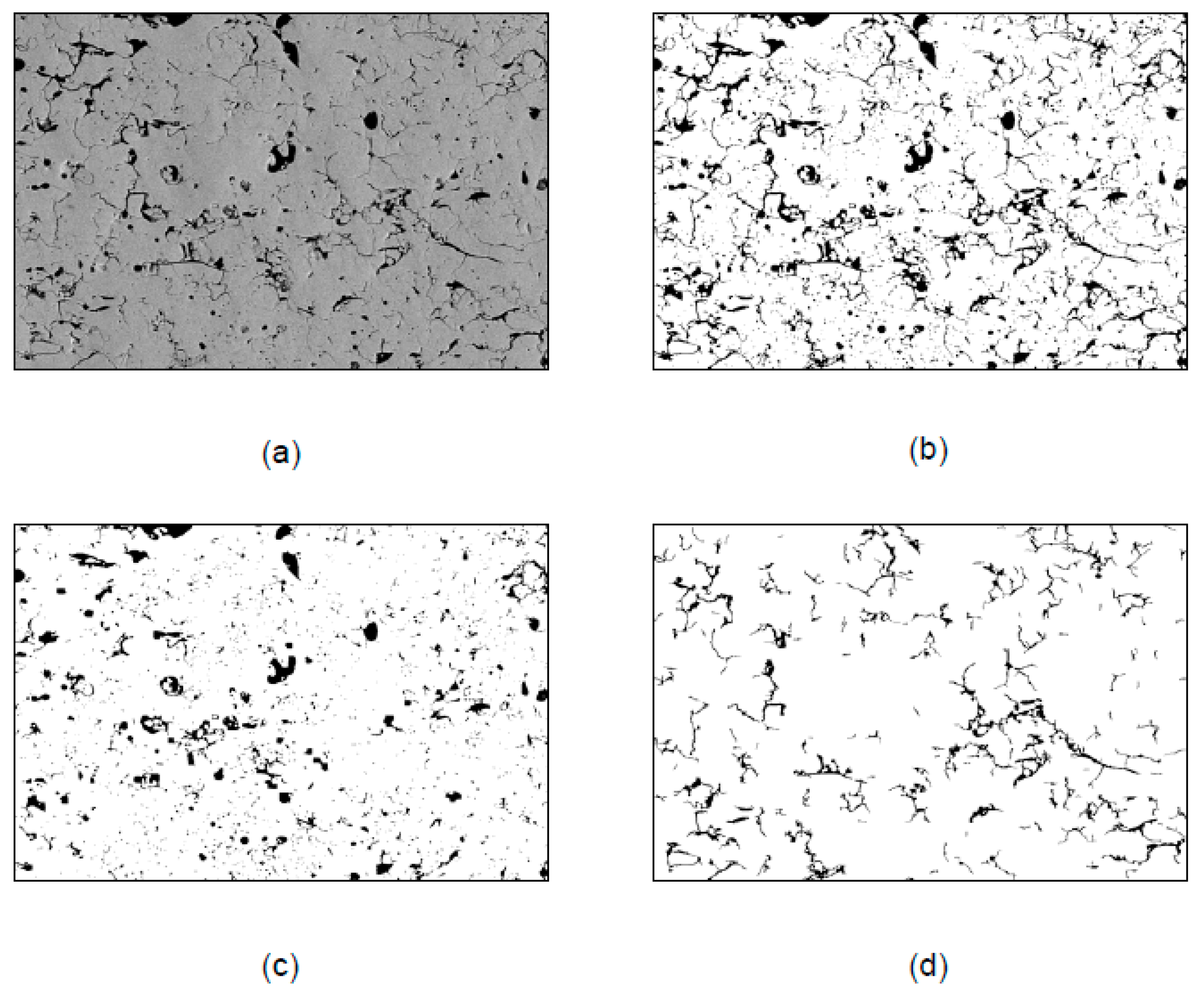The composition of these materials is (8YSZ) 8Y₂O₃-ZrO₂, (22MSZ) 22MgO-ZrO₂ and (25 CSZ) 25CeO₂-2.5Y₂O₃-ZrO₂. A single image of the cross-section is used to calculate the porosity content using Image J as shown in Figure 15. It should be noted that different images of the same coating (at different layer thickness) may produce different results for the porosity content. The porosity of sprayed coatings was evaluated using the Image J and is presented in

Table 6. Input parameters for the four-phase model [51].

Sample Materials	8YPSZ	22MSZ	25CSZ
Bulk thermal conductivity (W/(m.K))	2.8	2.2	2.8
Overall porosity (%) (As sprayed)	24.9 ± 0.08	16.4 ± 1.0	18.7 ± 0.05
Overall porosity (%) (Annealed)	19.7 ± 0.09	15.1 ± 0.7	13.9 ± 0.03
Open randomly oriented porosity (As sprayed)	0.9 ± 0.03	4.5 ± 0.08	3.9 ± 0.04
Open randomly oriented porosity (%) (Annealed)	5.2 ± 0.02	10.4 ± 0.05	3.4 ± 0.02
Microcracks (%) (As sprayed)	9.4 ± 0.05	5 ± 0.1	6.5 ± 0.04
Microcracks (%) (Annealed)	2.8 ± 0.01	3.3 ± 0.03	7.5 ± 0.05
Non-flat porosity (%) (As sprayed)	14.6 ± 0.06	9.6 ± 0.02	8.3 ± 0.04
Non-flat porosity (%) (Annealed)	11.7 ± 0.01	1.4 ± 0.04	5.4 ± 0.03

and this data is used as input parameters for the four-phase model. The porosity content of different coating materials is presented in Figure 16. The blue bars represent the porosity content of as-sprayed coatings and red bars represent the porosity content of heat-treated (annealed) coatings. A drop in the porosity content can be seen for the heat-treated coatings. This drop in the porosity is due to sintering of the coatings related to thermal cycling [17,82,83]. Further data are collected for three different forms of yttria-stabilized zirconia coatings. The results for porosity content are obtained for as-sprayed and annealed coatings using Image J. These YSZ coatings are FC (fused and crushed), AS (agglomerated and sintered) and HOSP (plasma densified hollow spheres) [80,84]. The porosity content of these YSZ coatings is presented in

Table 7. Calculated porosity for different YSZ samples using Image J.

YSZ Samples	Overall Porosity (%) (As-Sprayed)	Overall Porosity (%) (Annealed)
FC	21.3 ± 0.6	16.9 ± 0.3
AS	17.9 ± 0.1	16.1 ± 0.25
HOSP	19.0 ± 0.4	14.4 ± 0.2

. A graphical representation of the three different YSZ coatings is given in Figure 17 where the blue bars represent the porosity content of as-sprayed coatings and the red bars represent the porosity content of heat-treated annealed coatings.

The five-phase model is used to calculate the thermal conductivity of Molybdenum, 8YSZ, 22MSZ, 25CSZ, FC, AS and HOSP [50]. The data used in the calculation of thermal conductivity for the five-phase model and the results obtained after calculations can be obtained from

Table 8. Results obtained from the five-phase model for different materials [50].

Sample Material	Molybdenum	8YSZ	8YSZ (H.T)	22MSZ	22MSZ (H.T)	25CSZ	25CSZ (H.T)
Bulk thermal conductivity	142	2.8	2.8	2.2	2.2	2.8	2.8
Obtained thermal conductivity using the five-phase model	15.76 ± 0.05	1.18 ± 0.02	1.60 ± 0.03	1.14 ± 0.03	1.35 ± 0.02	1.175 ± 0.01	1.93 ± 0.04
Total porosity	50.5 ± 0.1	24.55 ± 0.09	20.7 ± 0.5	18.9 ± 0.12	16.8 ± 0.04	23.7 ± 0.08	13.9 ± 0.03
Open randomly oriented porosity (>100 nm)	9 ± 0.03	1.25 ± 0.04	5.2 ± 0.03	4.5 ± 0.02	10.4 ± 0.02	3.9 ± 0.01	5.1 ± 0.03
Microcracks (<100 nm)	13 ± 0.02	6.2 ± 0.01	2.8 ± 0.02	5 ± 0.01	3 ± 0.02	6.5 ± 0.04	1.9 ± 0.01
Non-flat porosity	13 ± 0.01	14.3 ± 0.03	11.7 ± 0.03	6.9 ± 0.04	1.4 ± 0.03	8.3 ± 0.05	3.8 ± 0.02
Penny shaped	15.5 ± 0.02	2.8 ± 0.01	1 ± 0.01	2.5 ± 0.02	2 ± 0.01	5 ± 0.04	3.1 ± 0.03

. Porosity content of the coating materials is presented in Figure 16 where the blue and red bars represent the porosity content of as-sprayed and annealed coatings respectively. The overall porosity is the combination of four different categories of pores, i.e., open randomly oriented pores, microcracks, non-flat porosity and penny-shaped cracks.

The thermal conductivity values obtained from the five-phase model for different as-sprayed and annealed coatings are presented in Figure 18. The overall porosity, porosity distribution among various contributing factors and the results obtained from the five-phase model are presented in

Table 9. Calculation of thermal conductivity for different YSZ samples using the five-phase model [50].

Sample Material	HOSP (As Sprayed)	HOSP (H.T)	FC (As Sprayed)	FC (H.T)	AS (As Sprayed)	AS (H.T)
Bulk thermal conductivity	2.8	2.8	2.8	2.8	2.8	2.8
Obtained thermal conductivity using the five-phase model	1.12 ± 0.03	1.36 ± 0.02	1.2 ± 0.05	1.79 ± 0.05	1.33 ± 0.03	1.56 ± 0.04
Total porosity	19 ± 0.01	14.4 ± 0.03	21.3 ± 0.02	16.9 ± 0.04	17.9 ± 0.04	16.1 ± 0.05
Open randomly oriented porosity (>100 nm)	3.6 ± 0.01	2.2 ± 0.01	6 ± 0.02	5.8 ± 0.01	4.99 ± 0.03	2 ± 0.01
Microcracks (<100 nm)	9.4 ± 0.03	8 ± 0.03	7.2 ± 0.03	2 ± 0.01	6.87 ± 0.01	4.8 ± 0.04
Non-flat porosity	3.5 ± 0.02	3 ± 0.01	3.1 ± 0.02	4.7 ± 0.02	4.05 ± 0.01	7.8 ± 0.03
Penny shaped	2.5 ± 0.01	1.2 ± 0.0	5 ± 0.04	4.4 ± 0.02	2 ± 0.01	1.5 ± 0.0

[50]. Blue bars represent the thermal conductivity of as-sprayed coatings and orange bars represent the thermal conductivity of annealed coatings. The increase in the thermal conductivity is attributed to sintering as small microcracks and vertical cracks or pores tends to diminish during the thermal cycling due to the expansion of coating material during heating [15,82].

7. Validation of the Calculated Results

To validate the results of the five-phase model, data are obtained from prior models, FEA models and experimental results for comparison with the five-phase model [4,7,37,45,50,51,58,80,82,83,84]. Comparison of results obtained from the five-phase model with results obtained from other models is drawn and the graphical representation of this comparison can be seen in Figure 19. Blue bars represent the thermal conductivity obtained from the five-phase model for composite materials, grey bars represent the thermal conductivity obtained from the four-phase model for composite materials and the orange bars represent the values obtained from experimental results. The value obtained from the experimental data in the case of 22MSZ (annealed) coating is much higher than the 22MSZ (as-sprayed). The bulk thermal conductivity of 22MSZ is 2.2 W/(m.K). The value obtained for heat-treated 22MSZ is near 4 W/(m.K), which is higher than the bulk thermal conductivity. Given the outlier nature of this point, it was assumed that this value was an error in the reference document.

A comparison is performed between the results obtained from the four-phase model, five-phase model and experimental results (

Table 10. Comparison of five-phase results with experimental results [50,62,78,80,82,83].

Sample	Experimental Thermal Conductivity		Simulated Thermal Conductivity Using the Five-Phase Model		Thermal Conductivity Obtained from the Four-Phase Model
	Before (H.T)	After (H.T)	Before (H.T)	After (H.T)	Before (H.T)	After (H.T)
8YSZ	1.2	1.62	1.18 ± 0.02	1.60 ± 0.03	1.0	1.68
22MSZ	1.1	4.37	1.14 ± 0.03	1.35 ± 0.03	1.2	1.37
25CSZ	1.19	2.05	1.175 ± 0.01	1.93 ± 0.04	1.13	1.68
Molybdenum	14.2–15.8	N/A	15.76 ± 0.02	N/A	N/A	N/A

) [50]. This comparison provides a better understanding of the results obtained since the five-phase model depicts the results better than the four-phase model. In

Table 11. Difference between results from the five-phase model and four-phase model.

Sample	Difference Between the Five-Phase Model and Four-Phase Model
8YSZ (As-sprayed)	15.25%
8YSZ (Annealed)	−5%
22MSZ (As-sprayed)	−5.2%
22MSZ (Annealed)	−1.48%
25CSZ (As-sprayed)	3.8%
25CSZ (Annealed)	12.95%

, the percentage difference between the results obtained from the five-phase model and four-phase model is calculated. A negative sign represents a percentage decrease in the values obtained using the five-phase model with respect to the four-phase model. In

Table 12. Thermal conductivity difference between the experimental results and the different models.

Sample	Thermal Conductivity Difference Between Experimental Values and Five-Phase Model	Thermal Conductivity Difference Between the Experimental Results Model and Four-Phase Model
8YSZ (As-sprayed)	−1.66%	−16.7%
8YSZ (Annealed)	−1.23%	3.7%
22MSZ (As-sprayed)	3.6%	9.1%
22MSZ (Annealed)	−69%	−68.6%
25CSZ (As-sprayed)	−1.26%	−5%
25CSZ (Annealed)	−5.85%	−18%
Molybdenum (As-sprayed)	−0.25% with maximum experimental value	N/A

, the difference between the thermal conductivity values obtained from experimental results and results from the five-phase model is calculated and presented in the second column. These results are compared with the difference between experimental thermal conductivity values and results from the four-phase model, which are presented in the third column. It can clearly be seen that the results obtained from the five-phase model are closer to the experimental values than those obtained from the four-phase model.

In Table 12, the percentage change in the difference obtained from experimental results and modelled results are presented. The negative sign represents the results that are below the experimental results. In most of the cases, the values obtained from the five-phase modelling are closer to the experimental values, neglecting the outlier results of 22MSZ. The results obtained using the proposed five-phase model are within 6% of experiment results [50].

In

Table 13. Comparison of the five-phase model with experimental and FEA results for three YSZ samples [50,80,84].

Samples	Experimental Thermal Conductivity (W/(m.K))	Five-Phase Model Thermal Conductivity (W/(m.K))	Thermal Conductivity Obtained from FEA (W/(m.K))
HOSP (As-sprayed)	1.10 ± (0.09)	1.12 ± (0.03)	1.32 ± (0.13)
HOSP (Annealed)	1.30 ± (0.1)	1.36 ± (0.02)	1.42 ± (0.14)
FC (As-sprayed)	1.23 ± (0.1)	1.2 ± (0.05)	1.56 ± (0.16)
FC (Annealed)	1.85 ± (0.15)	1.79 ± (0.05)	1.78 ± (0.18)
AS (As-sprayed)	1.12 ± (0.09)	1.33 ± (0.03)	1.75 ± (0.18)
AS (Annealed)	1.43 ± (0.11)	1.56 ± (0.04)	1.77 ± (0.18)

, thermal conductivity values obtained from three different YSZ coating materials are presented. These values were obtained from experimental results [51,80], FEA results [80] and from the five-phase modelling [50]. A comparison was performed between the values obtained for the different coatings.

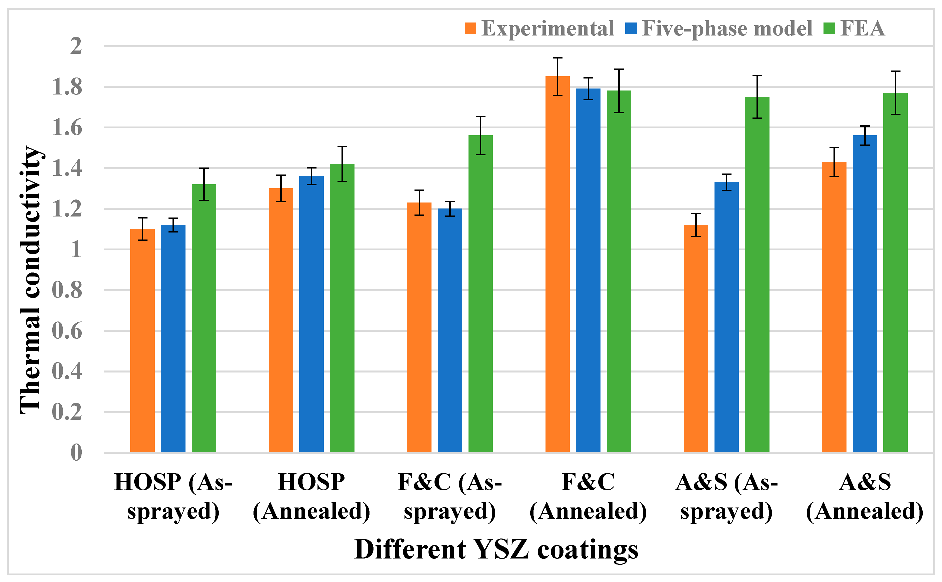
Table 13 and Figure 20 provide an overall comparison of the three different YSZ coatings, HOSP, FC and AS. Orange bars represent the experimental results, the blue bars represent the values obtained from the five-phase model and the green bars represent the values obtained from the FEA model. The FEA results are from the work of [80,84].

The values in

Table 14. Difference between the experimental and five-phase model results, and the difference between the FEA and five-phase model results.

Samples Obtained for Different YSZ Coatings	Difference between Thermal Conductivity Values from Experimental and Five-Phase Model	Difference between Thermal Conductivity Values from FEA and Five-Phase Model
HOSP (As-sprayed)	1.2%	−15.5%
HOSP (Annealed)	4.6%	−4.2%
FC (As-sprayed)	−2.4%	−23%
FC (Annealed)	−3.24%	0.5%
AS (As-sprayed)	18.7%	−24%
AS (Annealed)	9%	−11.8%

show the closeness of the values from the five-phase model to the experimental and FEA results. The negative percentage change represents values that are lower than the experimental and/or FEA results. It is concluded that the five-phase model predicts the thermal conductivity better than the FEA model [50].

8. Conclusions

A five-phase model to predict the thermal conductivity of thermal barrier coatings was developed in this work and validated against the results from the four-phase model, FEA model and experimental results. The presented model takes into consideration different types of pores/defects that are mostly present in a topcoat. The parameters used in the model were obtained from calculations performed during work, previous models and fitting parameters.

By comparing the simulated values with experimental results, it is shown that the proposed five-phase model can predict the thermal conductivity of ceramic coatings closer to the actual values. The proposed model uses real microstructure images and MIP results to obtain porosity content in the coatings to predict the thermal conductivity. The proposed model has the potential to predict microstructure-based properties and their relation.

The presence of different types of pores and cracks influences the overall thermal conductivity of the coatings. Microcracks present in the coating’s microstructure influence the thermal conductivity. The density of microcracks is affected by heat treatment due to the expansion of the coating material. Smaller cracks disappear in the coating due to sintering and lead to lower porosity content, which leads to an increase in thermal conductivity.

The thermal conductivity of the coatings was predicted based on the porosity content present in the top-coat. The five-phase model can predict the values of thermal conductivity within 6% of the experimental results. There is one exceptional case for 22MSZ, where the experimental result was much higher than the simulated value. In this specific case, the simulated results from both the four-phase and five-phase model were less than the experimental result. It is possible that a faulty data source that led to an error in the experimental results. Therefore, the data point for 22MSZ was treated as an outlier and neglected.

The results obtained from the five-phase model were in accordance with experimental results. The calculated results were better than those predicted by the FEA model. The difference in predicted value and experimental results were found to be within an acceptable error range. The modelling approach proposed in this paper could be used as a tool to model and measure the thermal conductivity of coatings and to design coatings with an optimized microstructure to enhance the performance of TBCs.