
Contributions to Management Strategies in the NE Atlantic Regarding the Life History and Population Structure of a Key Deep-Sea Fish (Mora Moro)

 , , , and
Abstract
:Simple Summary
Abstract
1. Introduction
2. Material and Methods
2.1. Datasets
2.2. Data Analyses
3. Results
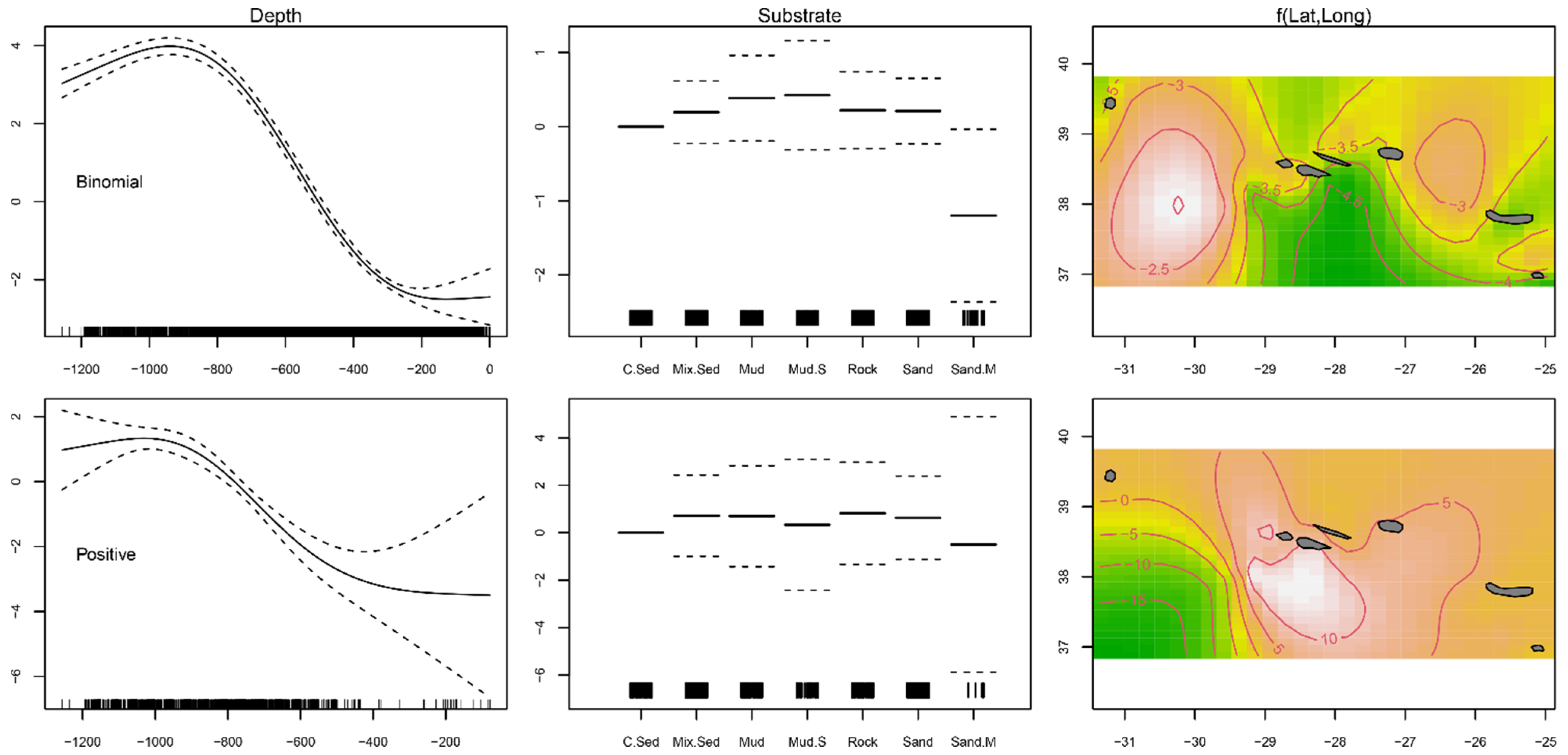
3.1. Habitat Preferences
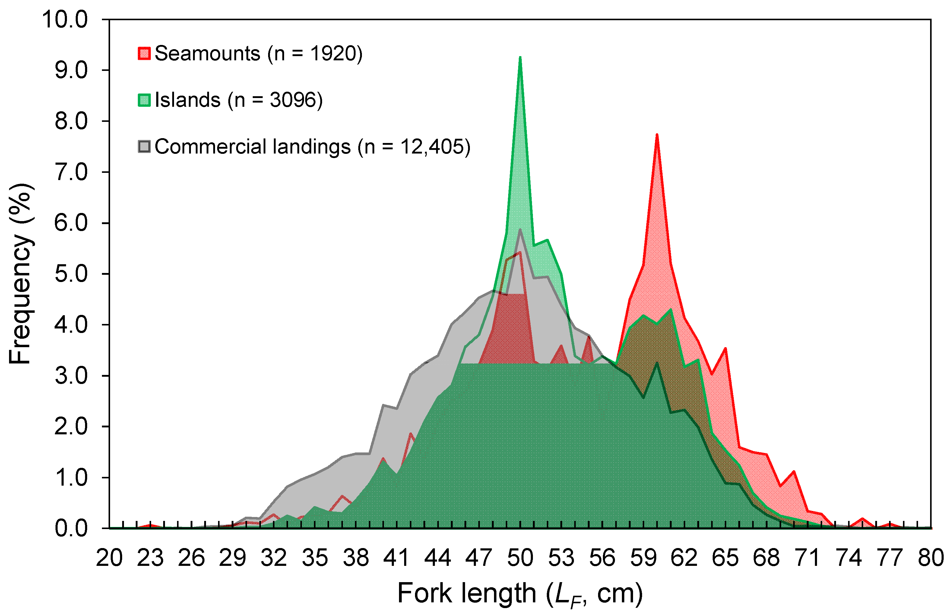
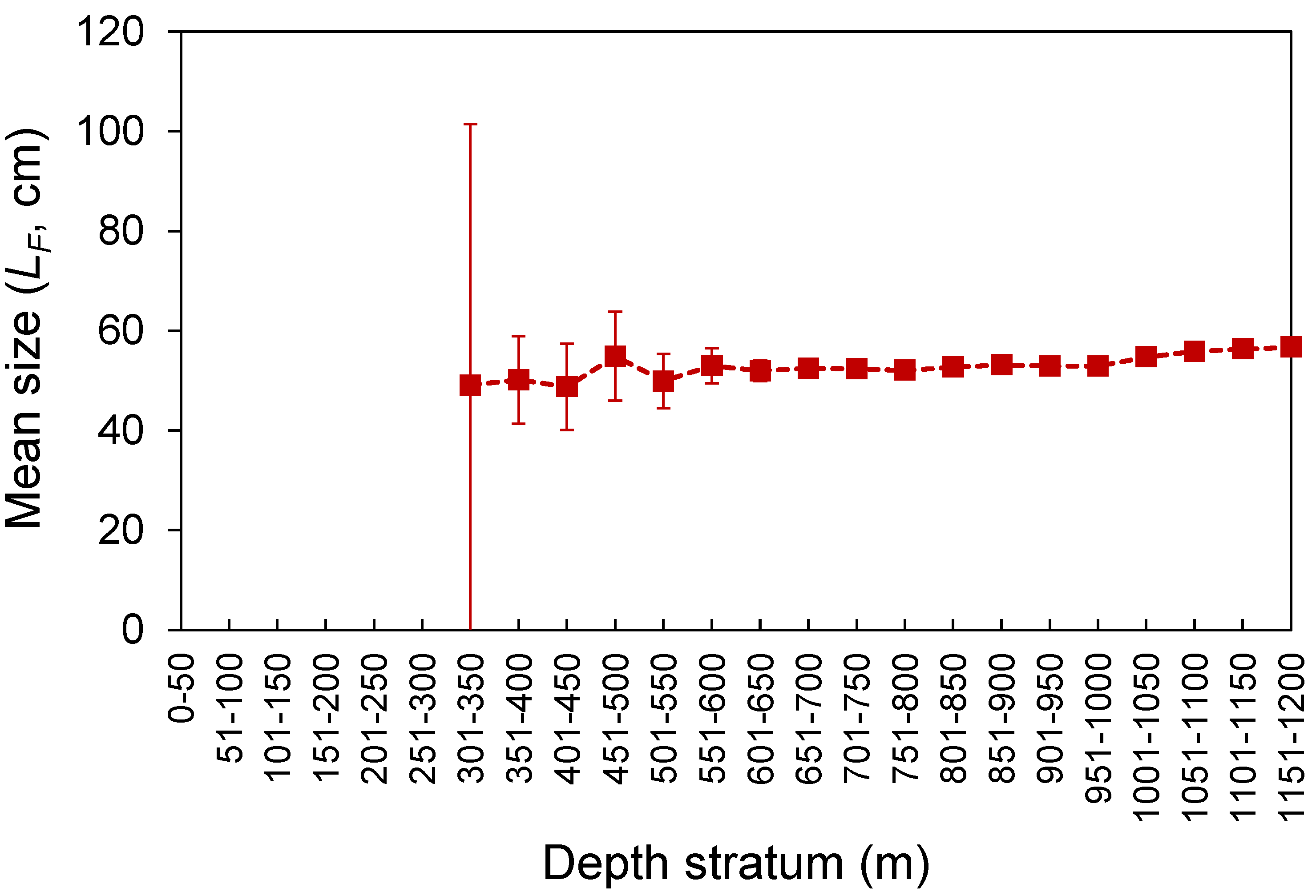
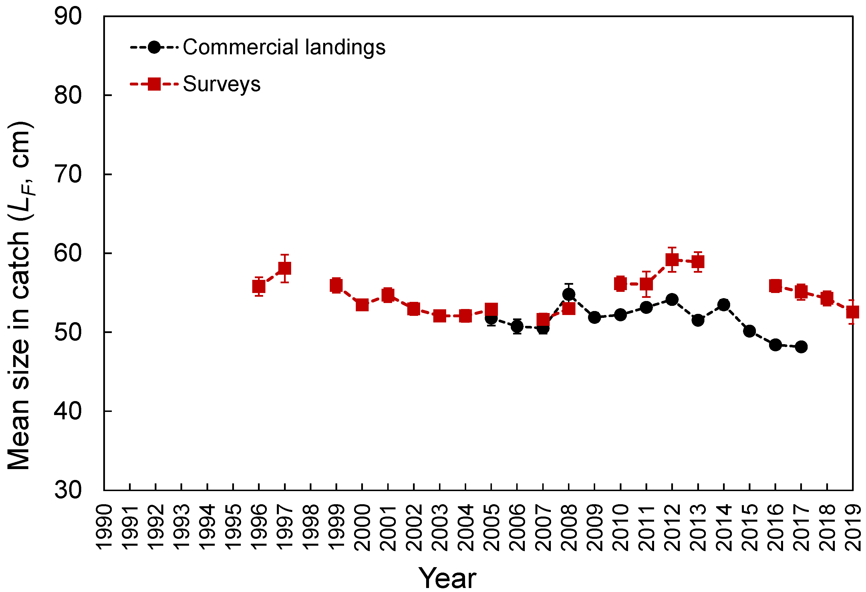
3.2. Size Structure
3.3. Growth Parameters
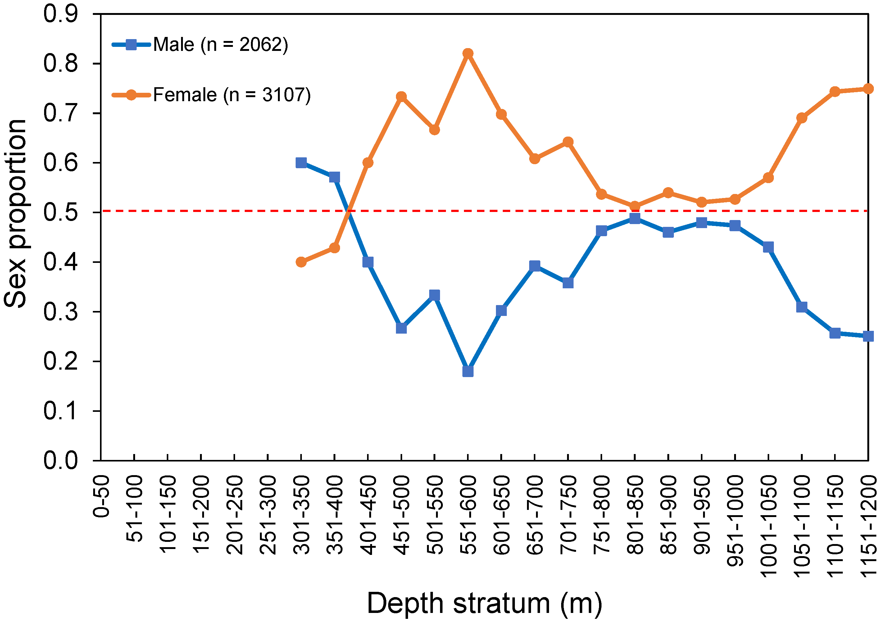
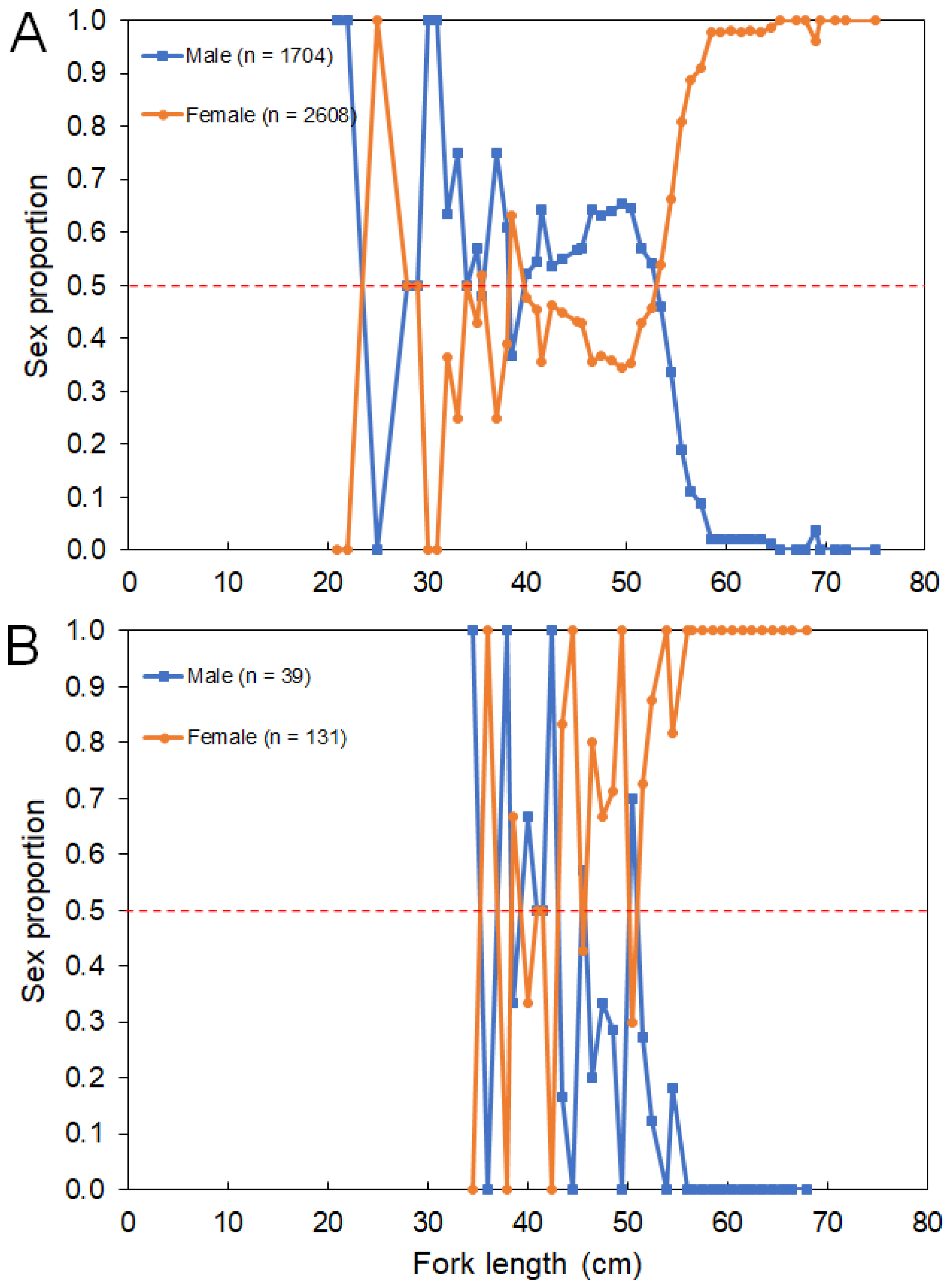
3.4. Sex Ratio
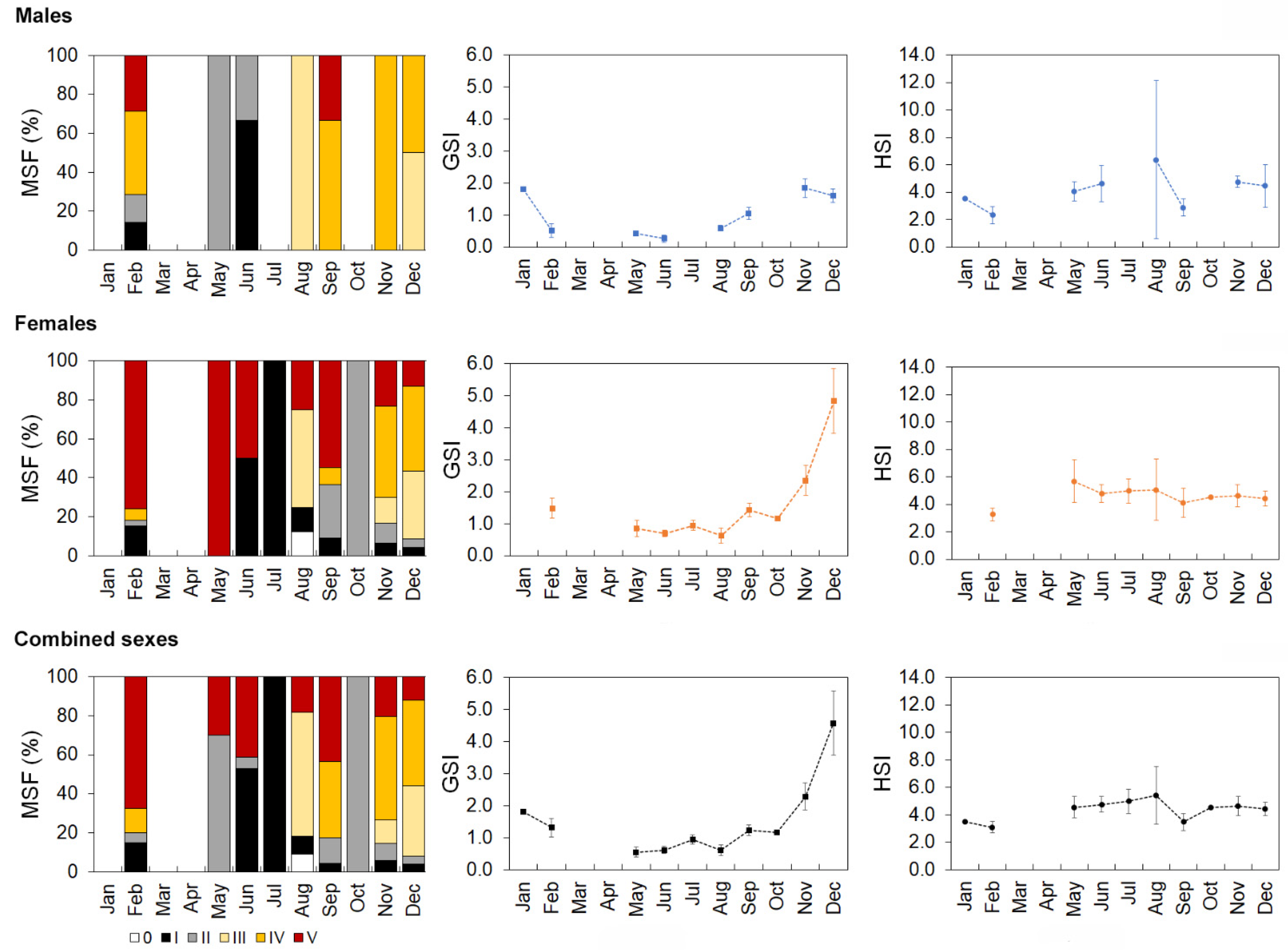
3.5. Reproduction
3.6. Mortality, Exploitation Rate, and Size at Capture
3.7. Catches and Landings
3.8. Fishing Effort
4. Discussion
5. Conclusions
Supplementary Materials
Author Contributions
Funding
Institutional Review Board Statement
Informed Consent Statement
Data Availability Statement
Acknowledgments
Conflicts of Interest
References
- Jennings, S.; Kaiser, M.J. The effects of fishing on marine ecosystems. Adv. Mar. Biol. 1998, 34, 201–212. [Google Scholar] [CrossRef]
- Food and Agriculture Organization of the United Nations (FAO). The State of World Fisheries and Aquaculture 2020; FAO: Rome, Italy, 2020; ISBN 9789251326923. [Google Scholar]
- Bennett, A.; Patil, P.; Kleisner, K.; Rader, D.; Virdin, J.; Basurto, X. Contribution of Fisheries to Food and Nutrition Security: Current Knowledge, Policy and Research; Duke University: Durham, NC, USA, 2018. [Google Scholar]
- Norse, E.A.; Brooke, S.; Cheung, W.W.L.; Clark, M.R.; Ekeland, I.; Froese, R.; Gjerde, K.M.; Haedrich, R.L.; Heppell, S.S.; Morato, T.; et al. Sustainability of deep-sea fisheries. Mar. Policy 2012, 36, 307–320. [Google Scholar] [CrossRef] [Green Version]
- Santos, R.V.S.; Silva, W.M.M.L.; Novoa-Pabon, A.M.; Silva, H.M.; Pinho, M.R. Long-term changes in the diversity, abundance and size composition of deep sea demersal teleosts from the Azores assessed through surveys and commercial landings. Aquat. Living Resour. 2019, 32, 25. [Google Scholar] [CrossRef] [Green Version]
- Cohen, D.M. Moridae. In Fishes of the North-Eastern Atlantic and the Mediterranean; Whitehead, P.J.P., Bauchot, M.-L., Hureau, J.-C., Nielson, J., Tortonese, E., Eds.; UNESCO: Paris, France, 1986; pp. 713–726. [Google Scholar]
- Santos, R.; Medeiros-Leal, W.; Pinho, M. Synopsis of biological, ecological and fisheries-related information on priority marine species in the Azores region. Arquipel. Life Mar. Sci. 2020, 1, 1–138. [Google Scholar]
- Froese, R.; Pauly, D. FishBase. Available online: https://www.fishbase.se/search.php (accessed on 5 March 2021).
- International Council for the Exploration of the Sea (ICES). Azores ecoregion—Ecosystem overview. In Report of the ICES Advisory Committee, 2020; ICES Advice 2020, Section 3.1; ICES: Reykjavik, Iceland, 2020. [Google Scholar]
- Açores. Ordinance No 101/2002 of October 2002 concerning the line fishing regulation in the Autonomous Region of the Azores. J. Of. Região Autónoma Açores I 2002, 43, 1132–1134. [Google Scholar]
- Açores. Ordinance No 50/2012 of April 2012 concerning the line fishing regulation in the Autonomous Region of the azores. J. Of. Região Autónoma Açores I 2012, 67, 1384–1393. [Google Scholar]
- Santos, R.; Medeiros-Leal, W.; Pinho, M. Stock assessment prioritization in the Azores: Procedures, current challenges and recommendations. Arquipel. Life Mar. Sci. 2020, 20–45. [Google Scholar]
- Fauconnet, L.; Pham, C.K.; Canha, A.; Afonso, P.; Diogo, H.; Machete, M.; Silva, H.M.; Vandeperre, F.; Morato, T. An overview of fisheries discards in the Azores. Fish. Res. 2019, 209, 230–241. [Google Scholar] [CrossRef]
- ICES Working Group on the Biology and Assessment of Deep-sea Fisheries Resources (WGDEEP). Report of the Working Group on the Biology and Assessment of Deep-sea Fisheries Resources (WGDEEP). ICES Sci. Rep. 2020, 2, 1–928. [Google Scholar] [CrossRef]
- Sparre, P.; Venema, S.C. Introduction To Tropical Fish Stock Assessment. Part 1: Manual—Part 2: Exercises; Food and Agriculture Organization of the United Nations (FAO): Rome, Italy, 1998; pp. 1–423. [Google Scholar]
- Uriarte, A.; Zarauz, L.; Aranda, M.; Santurtún, M.; Iriondo, A.; Berthou, P.; Castro, J.; Delayat, S.; Falcón, J.M.; García, J.; et al. Guidelines for the Definition of Operational Management Units; European Union: Brussels, Belgium, 2014. [Google Scholar]
- Staples, D.; Brainard, R.; Capezzuoli, S.; Funge-Smith, S.; Grose, C.; Heenan, A.; Hermes, R.; Maurin, P.; Moews, M.; O’Brien, C.; et al. Essential EAFM. Ecosystem Approach to Fisheries Management Training Course. Volume I—For Trainees; Food and Agriculture Organization of the United Nations (FAO): Bangkok, Thailand, 2014. [Google Scholar]
- Santos, R.V.S.; Novoa-Pabon, A.M.; Silva, H.M.; Pinho, M.R. Can we consider the stocks of alfonsinos Beryx splendens and Beryx decadactylus from the Azores a discrete fishery management unit? J. Fish Biol. 2019, 94. [Google Scholar] [CrossRef] [Green Version]
- Vieira, A.R.; Figueiredo, I.; Figueiredo, C.; Menezes, G.M. Age and growth of two deep-water fish species in the Azores Archipelago: Mora moro (Risso, 1810) and Epigonus telescopus (Risso, 1810). Deep. Res. Part II Top. Stud. Oceanogr. 2013, 98, 148–159. [Google Scholar] [CrossRef]
- Pinho, M.; Medeiros-Leal, W.; Sigler, M.; Santos, R.; Novoa-Pabon, A.; Menezes, G.; Silva, H. Azorean demersal longline survey abundance estimates: Procedures and variability. Reg. Stud. Mar. Sci. 2020, 39, 101443. [Google Scholar] [CrossRef]
- European Union. EU Council Regulation (EC) No 199/2008 of 25 February 2008 concerning the establishment of a Community framework for the collection, management and use of data in the fisheries sector and support for scientific advice regarding the Common Fisheries Policy. Off. J. Eur. Union L 2008, 60, 1–12. [Google Scholar]
- Deutsche Gesellschaft für Rechtsmedizin (DGRM). Work Plan for Data Collection in the Fisheries and Aquaculture Sectors; DGRM: Lisbon, Paortugal, 2016; pp. 1–43. [Google Scholar]
- Hastie, T.J.; Tibshirani, R.J. Generalized Additive Models; CRC Press: Boca Ratoon, FL, USA, 1990; Volume 43. [Google Scholar]
- Guisan, A.; Edwards, T.C.; Hastie, T. Generalized linear and generalized additive models in studies of species distributions: Setting the scene. Ecol. Modell. 2002, 157, 89–100. [Google Scholar] [CrossRef] [Green Version]
- Lo, N.C.; Jacobson, L.D.; Squire, J.L. Indices of Relative Abundance from Fish Spotter Data based on Delta-Lognornial Models. Can. J. Fish. Aquat. Sci. 1992, 49, 2515–2526. [Google Scholar] [CrossRef]
- Stefánsson, G. Analysis of groundfish survey abundance data: Combining the GLM and delta approaches. ICES J. Mar. Sci. 1996, 53, 577–588. [Google Scholar] [CrossRef]
- Wood, S.N. Fast stable restricted maximum likelihood and marginal likelihood estimation of semiparametric generalized linear models. J. R. Stat. Soc. 2011, 73, 3–36. [Google Scholar] [CrossRef] [Green Version]
- Wood, S.N.; Pya, N.; Safken, B. Smoothing parameter and model selection for general smooth models (with discussion). J. Am. Stat. Assoc. 2016, 111, 1548–1575. [Google Scholar] [CrossRef]
- Wood, S.N. Stable and efficient multiple smoothing parameter estimation for generalized additive models. J. Am. Stat. Assoc. 2004, 99, 673–686. [Google Scholar] [CrossRef] [Green Version]
- Wood, S.N. Generalized Additive Models: An Introduction with R, 2nd ed.; Chapman and Hall/CRC: London, UK, 2017. [Google Scholar]
- Wood, S.N. Thin-plate regression splines. J. R. Stat. Soc. 2003, 65, 95–114. [Google Scholar] [CrossRef]
- R Core Team. R: A Language and Environment for Statistical Computing; R Foundation for Statistical Computing: Vienna, Austria, 2020. [Google Scholar]
- Dag, O.; Dolgun, A.; Konar, N.M. Onewaytests: An R Package for One-Way Tests in Independent Groups Designs. R J. 2018, 10, 175–199. [Google Scholar] [CrossRef] [Green Version]
- von Bertalanffy, L. A quantitative theory of organic growth (inquires on growth laws. II). Hum. Biol. 1938, 10, 181–213. [Google Scholar]
- Schwamborn, R.; Mildenberger, T.K.; Taylor, M.H. Assessing sources of uncertainty in length-based estimates of body growth in populations of fishes and macroinvertebrates with bootstrapped ELEFAN. Ecol. Model. 2019, 393, 37–51. [Google Scholar] [CrossRef] [Green Version]
- Mildenberger, T.K.; Taylor, M.H.; Wolff, M. TropFishR: An R package for fisheries analysis with length-frequency data. Methods Ecol. Evol. 2017, 8, 1520–1527. [Google Scholar] [CrossRef] [Green Version]
- Taylor, M.H.; Mildenberger, T.K. Extending electronic length frequency analysis in R. Fish. Manag. Ecol. 2017, 24, 230–238. [Google Scholar] [CrossRef]
- Pauly, D.; Munro, J.L. Once more on the comparison of growth in fish and invertebrates. Fishbyte 1984, 2, 1–21. [Google Scholar]
- Holden, M.J.; Raitt, D.F.S. Manual of Fisheries Science. Part 2: Methods of Resource Investigation and Their Application; Food and Agriculture Organization of the United Nations (FAO): Rome, Italy, 1974; Volume 1. [Google Scholar]
- Torrejon-Magallanes, J. sizeMat: An R Package to Estimate Size at Sexual Maturity; R Foundation for Statistical Computing: Vienna, Austria, 2020. [Google Scholar]
- Gedamke, T.; Hoenig, J.M. Estimating Mortality from Mean Length Data in Nonequilibrium Situations, with Application to the Assessment of Goosefish. Trans. Am. Fish. Soc. 2006, 135, 476–487. [Google Scholar] [CrossRef]
- Then, A.Y.; Hoenig, J.M.; Huynh, Q.C. Estimating fishing and natural mortality rates, and catchability coefficient, from a series of observations on mean length and fishing effort. ICES J. Mar. Sci. 2017, 75, 610–620. [Google Scholar] [CrossRef]
- Gulland, J.A. The Fish Resources of the Ocean; Fishing News (Books) Ltd.: West Byfleet, UK, 1971. [Google Scholar]
- Ortiz, M.; Arocha, F. Alternative error distribution models for standardization of catch rates of non-target species from a pelagic longline fishery: Billfish species in the Venezuelan tuna longline fishery. Fish. Res. 2004, 70, 275–297. [Google Scholar] [CrossRef]
- Zuur, A.F.; Ieno, E.N. Beginner’s Guide to Zero-Inflated Models with R; Highland Statistics Ltd.: Newburgh, UK, 2016; ISBN 978-0-9571741-8-4. [Google Scholar]
- Lenth, R. V Least-Squares Means: The {R} Package {lsmeans}. J. Stat. Softw. 2016, 69, 1–33. [Google Scholar] [CrossRef] [Green Version]
- Pante, E.; Simon-Bouhet, B. marmap: A Package for Importing, Plotting and Analyzing Bathymetric and Topographic Data in R. PLoS ONE 2013, 8, e73051. [Google Scholar] [CrossRef] [PubMed]
- Santos, R.; Medeiros-Leal, W.; Novoa-Pabon, A.; Silva, H.; Pinho, M. Demersal fish assemblages on seamounts exploited by fishing in the Azores (NE Atlantic). J. Appl. Ichthyol. 2021, 37, 198–215. [Google Scholar] [CrossRef]
- Bianchi, G. Demersal Assemblages of Tropical Continental Shelves. Ph.D. Thesis, University of Bergen, Bergen, Norway, 1992. [Google Scholar]
- Gaertner, J.C. Seasonal organization patterns of demersal assemblages in the Gulf of Lions (north-western Mediterranean Sea). J. Mar. Biol. Assoc. 2000, 80, 777–783. [Google Scholar] [CrossRef]
- Parra, H.E.; Pham, C.K.; Menezes, G.M.; Rosa, A.; Tempera, F.; Morato, T. Predictive modeling of deep-sea fish distribution in the Azores. Deep. Res. Part II Top. Stud. Oceanogr. 2017, 145, 49–60. [Google Scholar] [CrossRef]
- Fernandez-Arcaya, U.; Rotllant, G.; Ramirez-Llodra, E.; Recasens, L.; Aguzzi, J.; Flexas, M.M.; Sanchez-Vidal, A.; López-Fernández, P.; García, J.A.; Company, J.B. Reproductive biology and recruitment of the deep-sea fish community from the NW Mediterranean continental margin. Prog. Oceanogr. 2013, 118, 222–234. [Google Scholar] [CrossRef]
- Santos, R.; Pabon, A.; Silva, W.; Silva, H.; Pinho, M. Population structure and movement patterns of blackbelly rosefish in the NE Atlantic Ocean (Azores archipelago). Fish. Oceanogr. 2020, 29. [Google Scholar] [CrossRef]
- Gordon, J.D.M.; Mauchline, J. The distribution and diet of the dominant, slope-dwelling eel, Synaphobranchus kaupi, of the Rockall Trough. J. Mar. Biol. Assoc. 1996, 76, 493–503. [Google Scholar] [CrossRef]
- Capezzuto, F.; Carlucci, R.; Maiorano, P.; Sion, L.; Battista, D.; Giove, A.; Indennidate, A.; Tursi, A.; D’Onghia, G. The bathyal benthopelagic fauna in the north-western Ionian Sea: Structure, patterns and interactions. Chem. Ecol. 2010, 26, 199–217. [Google Scholar] [CrossRef]
- Stefanescu, C.; Rucabado, J.; Lloris, D. Depth-size trends in western Mediterranean demersal deep-sea fishes. Mar. Ecol. Prog. Ser. 1992, 81, 205–213. [Google Scholar] [CrossRef]
- Moranta, J.; Palmer, M.; Massutí, E.; Stefanescu, C.; Morales-Nin, B. Body fish size tendencies within and among species in the deep-sea of the western Mediterranean. Sci. Mar. 2004, 68, 141–152. [Google Scholar] [CrossRef] [Green Version]
- Rotllant, G.; Moranta, J.; Massutí, E.; Sardà, F.; Morales-Nin, B. Reproductive biology of three gadiform fish species through the Mediterranean deep-sea range (147–1850 m). Sci. Mar. 2002, 66, 157–166. [Google Scholar] [CrossRef] [Green Version]
- MacGibbon, D.J. Fishery Characterisation and Standardised CPUE Analyses for Ribaldo, Mora moro (Risso, 1810) (Moridae), 1989–1990 to 2012–13; New Zealand Government: Wellington, New Zealand, 2015. [Google Scholar]
- Fossen, I.; Bergstad, O.A. Distribution and biology of blue hake, Antimora rostrata (Pisces: Moridae), along the mid-Atlantic Ridge and off Greenland. Fish. Res. 2006, 82, 19–29. [Google Scholar] [CrossRef]
- D’Onghia, G.; Indennidate, A.; Giove, A.; Savini, A.; Capezzuto, F.; Sion, L.; Vertino, A.; Maiorano, P. Distribution and behaviour of deep-sea benthopelagic fauna observed using towed cameras in the Santa Maria di Leuca cold-water coral province. Mar. Ecol. Prog. Ser. 2011, 443, 95–110. [Google Scholar] [CrossRef] [Green Version]
- Dallarés, S.; Constenla, M.; Padrós, F.; Cartes, J.E.; Solé, M.; Carrassón, M. Parasites of the deep-sea fish Mora moro (Risso, 1810) from the NW Mediterranean Sea and relationship with fish diet and enzymatic biomarkers. Deep. Res. Part I Oceanogr. Res. Pap. 2014, 92, 115–126. [Google Scholar] [CrossRef]
- ICES Advisory Committee. Report of the Workshop for Maturity Staging Chairs (WKMATCH); ICES: Copenhagen, Denmark, 2014; pp. 1–57. [Google Scholar]
- Silva, H.M.; Pinho, M.R. Small-Scale Fishing on Seamounts. In Seamounts: Ecology, Fisheries & Conservation; John Wiley & Sons, Ltd.: Hoboken, NJ, USA, 2007; pp. 333–360. ISBN 9780470691953. [Google Scholar]
- Froese, R.; Binohlan, C. Empirical relationships to estimate asymptotic length, length at first maturity and length at maximum yield per recruit in fishes, with a simple method to evaluate length frequency data. J. Fish Biol. 2000, 56, 758–773. [Google Scholar] [CrossRef]
- Pauly, D. Theory and Management of Tropical Multi-Species Stocks: A Review, with Emphasis on the Southeast Asian Demersal Fisheries; International Center for Living Aquatic Resources Management: Manila, Philippines, 1979; Volume 1. [Google Scholar]
- Santos, R.; Novoa-Pabon, A.; Silva, H.; Pinho, M. Elasmobranch species richness, fisheries, abundance and size composition in the Azores archipelago (NE Atlantic). Mar. Biol. Res. 2020, 16. [Google Scholar] [CrossRef]
- Medeiros-Leal, W.; Santos, R.; Novoa-Pabon, A.; Silva, H.; Pinho, M. Population structure of the European conger Conger conger from the mid-North Atlantic Ocean inferred from bathymetric distribution, length composition and movement patterns analyses. Fish. Manag. Ecol. 2021. [Google Scholar] [CrossRef]
- Santos, R.; Medeiros-Leal, W.; Novoa-Pabon, A.; Pinho, M.; Isidro, E.; Melo, O.; Santos, R.; Medeiros-Leal, W.; Novoa-Pabon, A.; Pinho, M.; et al. Unraveling distributional patterns and life-history traits of a deep-water shrimp Plesionika edwardsii (Decapoda, Pandalidae) under unexploited virgin conditions: A benchmark for fisheries management. Nauplius 2021, 29. [Google Scholar] [CrossRef]
- Santos, R.; Pinho, M.; Melo, O.; Gonçalves, J.; Leocádio, A.; Aranha, A.; Menezes, G.; Isidro, E. Biological and ecological aspects of the deep-water red crab populations inhabiting isolated seamounts to the west of the Azores (Mid-Atlantic Ridge). Fish. Oceanogr. 2019, 28. [Google Scholar] [CrossRef]
- Thorson, J.T.; Munch, S.B.; Cope, J.M.; Gao, J. Predicting life history parameters for all fishes worldwide. Ecol. Appl. 2017, 27, 2262–2276. [Google Scholar] [CrossRef]
- Then, A.Y.; Hoenig, J.M.; Hall, N.G.; Hewitt, D.A. Evaluating the predictive performance of empirical estimators of natural mortality rate using information on over 200 fish species. ICES J. Mar. Sci. 2014, 72, 82–92. [Google Scholar] [CrossRef]


| Family | Link Function | Formula | Adjusted R2 | Deviance Explained | |||||
|---|---|---|---|---|---|---|---|---|---|
| Binomial | logit | RPN.Bi ~ s (Longitude, Latitude) + s (Depth, k = 4) + Substrate | 0.442 | 45.40% | |||||
| Gaussian | identity | RPN ~ s (Longitude, Latitude) + s (Depth, k = 4) + Substrate | 0.223 | 23.90% | |||||
| Binomial | Gaussian | ||||||||
| Parametric coefficients | |||||||||
| Estimate | Std. Error | z Value | Pr(>|z|) | Estimate | Std. Error | z Value | Pr(>|z|) | ||
| (Intercept) | −3.131 | 0.219 | −14.329 | <0.001 | (Intercept) | 3.301 | 0.820 | 4.028 | <0.001 |
| SubstrateMix.Sed | 0.195 | 0.210 | 0.928 | 0.354 | SubstrateMix.Sed | 0.718 | 0.855 | 0.840 | 0.401 |
| SubstrateMud | 0.384 | 0.289 | 1.331 | 0.183 | SubstrateMud | 0.695 | 1.062 | 0.654 | 0.513 |
| SubstrateMud.S | 0.425 | 0.368 | 1.154 | 0.248 | SubstrateMud.S | 0.334 | 1.379 | 0.242 | 0.809 |
| SubstrateRock | 0.223 | 0.259 | 0.858 | 0.391 | SubstrateRock | 0.818 | 1.078 | 0.759 | 0.448 |
| SubstrateSand | 0.211 | 0.221 | 0.955 | 0.340 | SubstrateSand | 0.633 | 0.876 | 0.722 | 0.470 |
| SubstrateSand.M | −1.199 | 0.583 | −2.059 | 0.040 | SubstrateSand.M | −0.496 | 2.693 | −0.184 | 0.854 |
| Approximate Significance of Smooth Terms | |||||||||
| edf | Ref. df | Chi. sq | p-Value | edf | Ref. df | Chi. sq | p-Value | ||
| s (Longitude, Latitude) | 24.430 | 27.530 | 74.540 | <0.001 | s (Longitude, Latitude) | 27.832 | 28.893 | 16.840 | <0.001 |
| s (Depth) | 2.990 | 3.000 | 1610.380 | <0.001 | s (Depth) | 2.866 | 2.987 | 25.990 | <0.001 |
| Parameters | Method | Estimates | Lower | Upper |
|---|---|---|---|---|
| Asymptotic length (L∞; cm LF) | ELEFAN_GA_Boot [35] | 77.68 | 75.17 a | 79.61 a |
| Growth coefficient (k; year−1) | ELEFAN_GA_Boot [35] | 0.07 | 0.05 a | 0.08 a |
| Growth performance index (⏀) | ELEFAN_GA_Boot [35] | 2.63 | 2.54 a | 2.71a |
| Natural mortality (M; year−1) | [42] | 0.16 | −0.03 b | 0.35 b |
| Total mortality (Z; year−1) | [41] | 0.21 | 0.20 c | 0.22 c |
| Fishing mortality (F; year−1) | [42] | 0.05 | 0.03 b | 0.07 b |
| Exploitation rate (E) | [43] | 0.24 | ||
| Catchability coefficient (q) | [42] | 0.03 | −0.08 b | 0.14 b |
| Length of full selectivity (Lc; cm LF) | [41] | 50.0 |
Publisher’s Note: MDPI stays neutral with regard to jurisdictional claims in published maps and institutional affiliations. |
© 2021 by the authors. Licensee MDPI, Basel, Switzerland. This article is an open access article distributed under the terms and conditions of the Creative Commons Attribution (CC BY) license (https://creativecommons.org/licenses/by/4.0/).
Share and Cite
Santos, R.; Medeiros-Leal, W.; Crespo, O.; Novoa-Pabon, A.; Pinho, M. Contributions to Management Strategies in the NE Atlantic Regarding the Life History and Population Structure of a Key Deep-Sea Fish (Mora Moro). Biology 2021, 10, 522. https://doi.org/10.3390/biology10060522
Santos R, Medeiros-Leal W, Crespo O, Novoa-Pabon A, Pinho M. Contributions to Management Strategies in the NE Atlantic Regarding the Life History and Population Structure of a Key Deep-Sea Fish (Mora Moro). Biology. 2021; 10(6):522. https://doi.org/10.3390/biology10060522
Chicago/Turabian StyleSantos, Régis, Wendell Medeiros-Leal, Osman Crespo, Ana Novoa-Pabon, and Mário Pinho. 2021. "Contributions to Management Strategies in the NE Atlantic Regarding the Life History and Population Structure of a Key Deep-Sea Fish (Mora Moro)" Biology 10, no. 6: 522. https://doi.org/10.3390/biology10060522