
Overlap and Segregation among Multiple 3D Home Ranges: A Non-Pairwise Metric with Demonstrative Application to the Lesser Kestrel Falco naumanni


Abstract
:Simple Summary
Abstract
1. Introduction
2. Materials and Methods
2.1. Study Species and Study Area
2.2. Tagging of Birds
2.3. Data Preparation
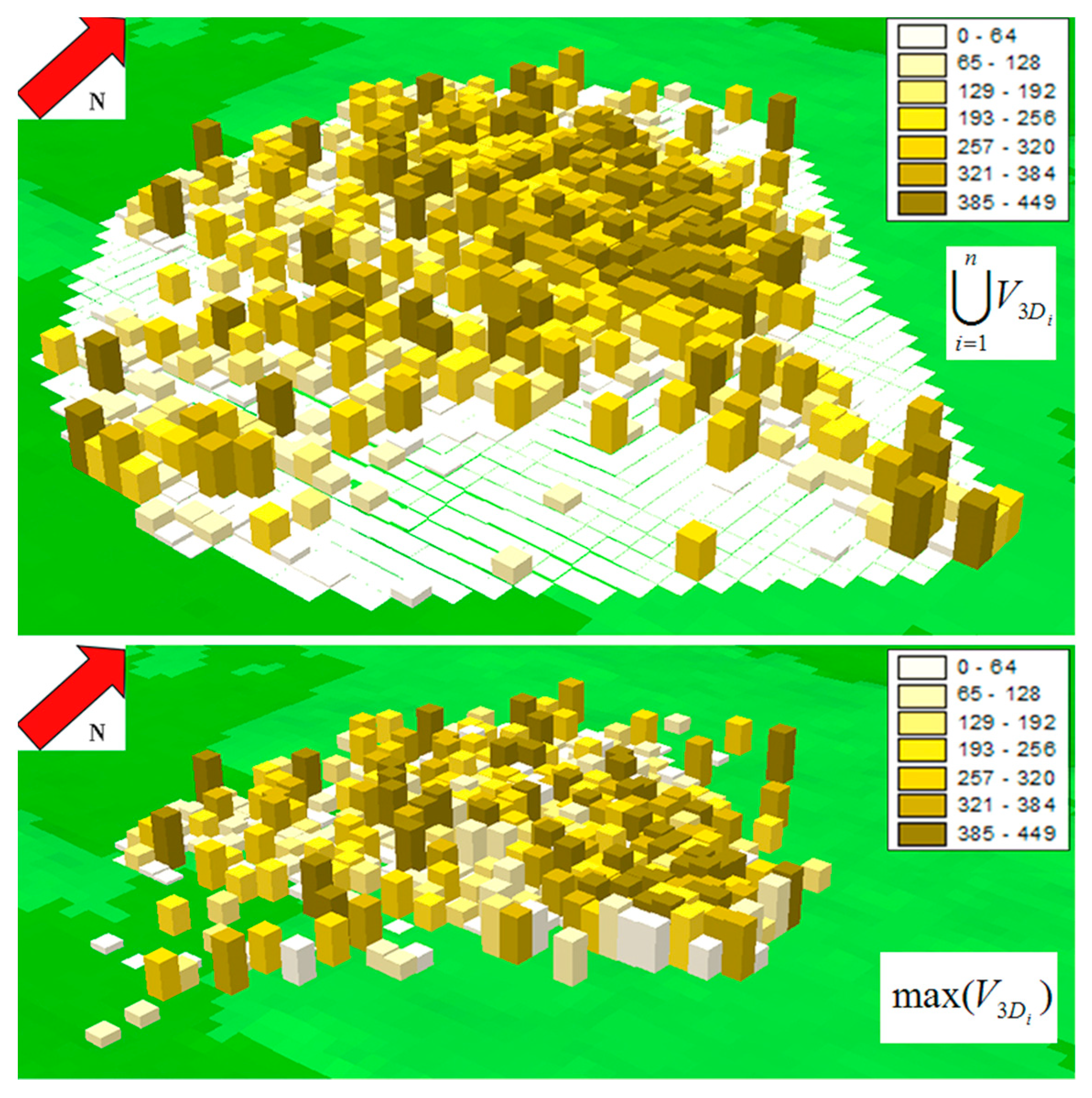
2.4. 3D Volumetric Home Ranges
2.5. 3D Home Range Overlap
3. Results
4. Discussion
4.1. Applications to Tracking Studies
4.2. Mathematical Properties of the Proposed Metrics
5. Conclusions
Author Contributions
Funding
Institutional Review Board Statement
Informed Consent Statement
Data Availability Statement
Acknowledgments
Conflicts of Interest
References
- Heide-Jørgensen, M.P.; Laidre, K.L.; Litovka, D.; Villum Jensen, M.; Grebmeier, J.M.; Sirenko, B.I. Identifying gray whale (Eschrichtius robustus) foraging grounds along the Chukotka peninsula, Russia, using satellite telemetry. Polar Biol. 2012, 35, 1035–1045. [Google Scholar] [CrossRef]
- Börger, L.; Dalziel, B.D.; Fryxell, J.M. Are there general mechanisms of animal home range behaviour? A review and prospects for future research. Ecol. Lett. 2008, 11, 637–650. [Google Scholar] [CrossRef] [PubMed]
- Marzluff, J.M.; Millspaugh, J.J.; Hurvitz, P.; Handcock, M.S. Relating resources to a probabilistic measure of space use: Forest fragments and Steller’s jays. Ecology 2004, 85, 1411–1427. [Google Scholar] [CrossRef] [Green Version]
- Lebsock, A.A.; Burdett, C.L.; Darden, S.K.; Dabelsteen, T.; Antolin, M.F.; Crooks, K.R. Space use and territoriality in swift foxes (Vulpes velox) in Northeastern Colorado. Can. J. Zool. 2012, 90, 337–344. [Google Scholar] [CrossRef]
- Avgar, T.; Mosser, A.; Brown, G.S.; Fryxell, J.M. Environmental and individual drivers of animal movement patterns across a wide geographical gradient. J. Anim. Ecol. 2013, 82, 96–106. [Google Scholar] [CrossRef] [PubMed]
- Jonsson, P.; Hartikainen, T.; Koskela, E.S.A.; Mappes, T. Determinants of reproductive success in voles: Space use in relation to food and litter size manipulation. Evol. Ecol. 2002, 16, 455–467. [Google Scholar] [CrossRef]
- Burt, W.H. Territoriality and home range concepts as applied to mammals. J. Mammal. 1943, 24, 346–352. [Google Scholar] [CrossRef]
- Tracey, J.A.; Sheppard, J.; Zhu, J.; Wei, F.; Swaisgood, R.R.; Fisher, R.N. Movement-based estimation and visualization of space use in 3Dfor wildlife ecology and conservation. PLoS ONE 2014, 9, e101205. [Google Scholar] [CrossRef] [Green Version]
- Keating, K.A.; Cherry, S. Modeling utilization distributions in space and time. Ecology 2009, 90, 1971–1980. [Google Scholar] [CrossRef]
- Simpfendorfer, C.A.; Olsen, E.M.; Heupel, M.R.; Moland, E. Three-dimensional kernel utilization distributions improve estimates of space use in aquatic animals. Can. J. Fish. Aquat. Sci. 2012, 69, 565–572. [Google Scholar] [CrossRef]
- Duong, T. ks: Kernel density estimation and kernel discriminant analysis for multivariate data in R. J. Stat. Softw. 2007, 21, 1–16. [Google Scholar] [CrossRef] [Green Version]
- Ferrarini, A.; Giglio, G.; Pellegrino, S.C.; Frassanito, A.; Gustin, M. A new methodology for computing birds’ 3D home ranges. Avian Res. 2018, 9, 19. [Google Scholar] [CrossRef] [Green Version]
- Cooper, N.W.; Sherry, T.W.; Marra, P.P. Modeling three-dimensional space use and overlap in birds. Auk 2014, 131, 681–693. [Google Scholar] [CrossRef]
- Ferrarini, A.; Giglio, G.; Pellegrino, S.C.; Gustin, M. Measuring the Degree of Overlap and Segregation among Multiple Probabilistic Home Ranges: A New Index with Illustrative Application to the Lesser Kestrel Falco naumanni. Animals 2021, 11, 2913. [Google Scholar] [CrossRef]
- Van Winkle, W. Comparison of several probabilistic home-range models. J. Wildl. Manag. 1975, 39, 118–123. [Google Scholar] [CrossRef]
- Ferrarini, A.; Giglio, G.; Pellegrino, S.C.; Gustin, M. A new general index of home range overlap and segregation: The Lesser Kestrel in Southern Italy as a case study. Avian Res. 2021, 12, 4. [Google Scholar] [CrossRef]
- BirdLife International. Species Factsheet: Falco naumanni. 2017. Available online: www.birdlife.org (accessed on 9 June 2022).
- La Gioia, G.; Melega, L.; Fornasari, L. Piano d′Azione Nazionale per il Grillaio (Falco naumanni); MATTM-ISPRA: Roma, Italy, 2017. [Google Scholar]
- TechnoSmart. GiPSy-4 Manual. Micro GPS Data-Logger for Tracking Free-Moving Animals; TechnoSmart: Roma, Italy, 2012. [Google Scholar]
- ESRI (Environmental Systems Research Institute). Using ArcView GIS; ESRI Press: Redlands, CA, USA, 1996. [Google Scholar]
- Kenward, R. Wildlife Radio Tagging; Academic Press Inc.: London, UK, 1987. [Google Scholar]
- Worton, B. Kernel methods for estimating the utilization distribution in home-range studies. Ecology 1989, 70, 164–168. [Google Scholar] [CrossRef]
- Hurlbert, S.H. The measurement of niche overlap and some relatives. Ecology 1978, 59, 67–77. [Google Scholar] [CrossRef]
- Fieberg, J.; Kochanny, C.O. Quantifying home-range overlap: The importance of the utilization distribution. J. Wildl. Manag. 2005, 69, 1346–1359. [Google Scholar] [CrossRef]
- Belant, J.L.; Millspaugh, J.J.; Martin, J.A.; Gitzen, R.A. Multi-dimensional space use: The final frontier. Front. Ecol. Environ. 2012, 10, 11–12. [Google Scholar] [CrossRef]
- Ferrarini, A.; Giglio, G.; Pellegrino, S.C.; Frassanito, A.; Gustin, M. First evidence of mutually exclusive home ranges in the two main colonies of Lesser Kestrels in Italy. Ardea 2018, 106, 85–89. [Google Scholar] [CrossRef]
- Bispo, R.; Bernardino, J.; Marques, T.A.; Pestana, D. Modeling carcass removal time and estimation of a scavenging correction factor for avian mortality assessment in wind farms using parametric survival analysis. Environ. Ecol. Stat. 2013, 20, 147–165. [Google Scholar] [CrossRef]
- Costantini, A.; Gustin, M.; Ferrarini, A.; Dell’omo, G. Estimates of avian collision with power lines and carcass disappearance across differing environments. Anim. Conserv. 2017, 20, 173–181. [Google Scholar] [CrossRef] [Green Version]
- Ferrarini, A.; Giglio, G.; Pellegrino, S.C.; Gustin, M. A community-level approach to species conservation: A case study of Falco naumanni in Southern Italy. Diversity 2022, 14, 566. [Google Scholar] [CrossRef]
- Laver, P.N.; Kelly, M.J. A critical review of home range studies. J. Wildl. Manage. 2008, 72, 290–298. [Google Scholar] [CrossRef]


| GPS | Sex | Weight | Start Date | End Date | Number of |
|---|---|---|---|---|---|
| ID | (g) | of Tracking | of Tracking | GPS Points | |
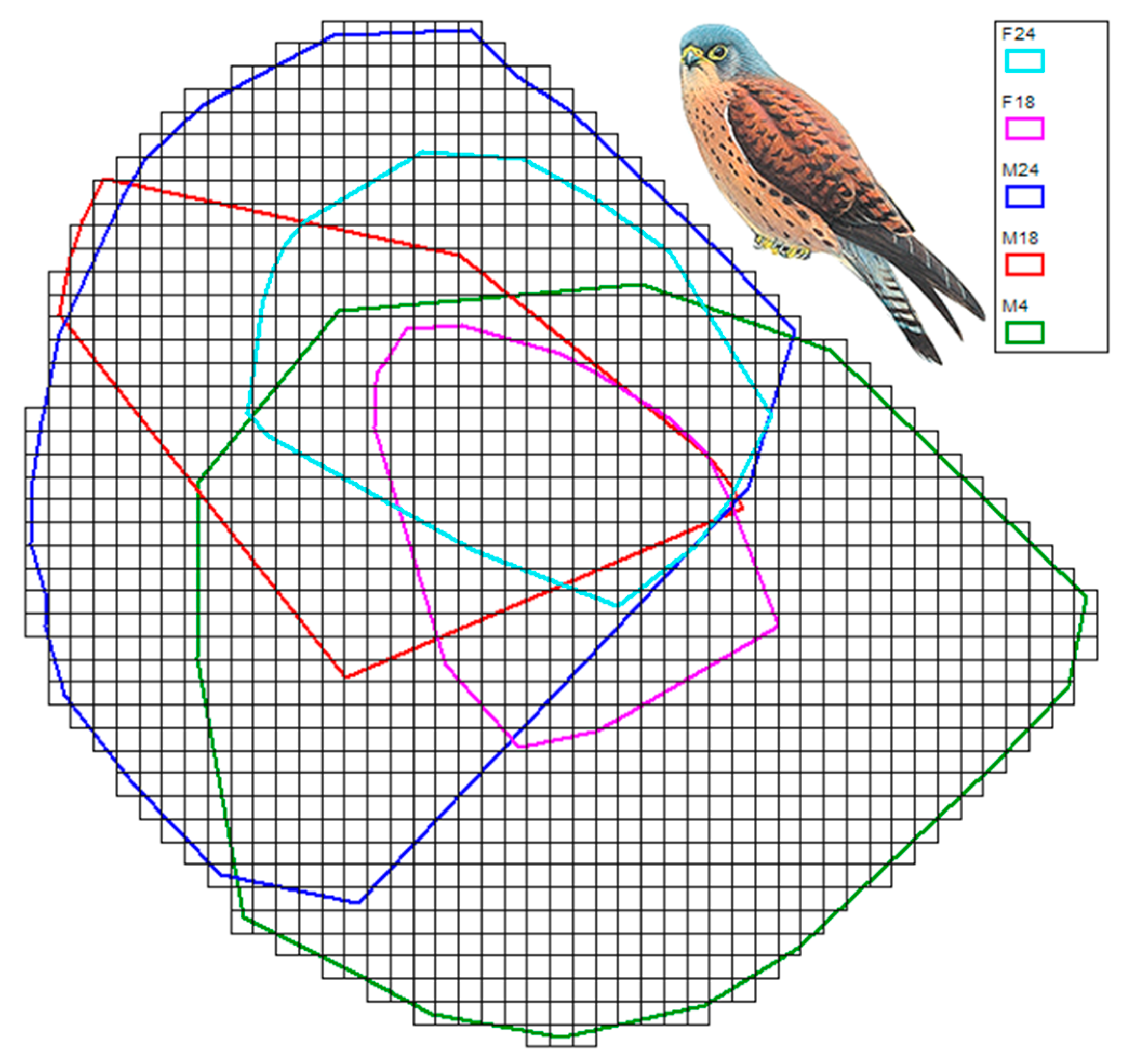
| F18 | F | 155 | 13 June 2017 | 16 June 2017 | 1375 |
| F24 | F | 126 | 22 June 2017 | 29 June 2017 | 3311 |
| M4 | M | 128 | 16 June 2017 | 22 June 2017 | 2765 |
| M18 | M | 135 | 13 June 2017 | 16 June 2017 | 1417 |
| M24 | M | 126 | 22 June 2017 | 29 June 2017 | 3213 |
| Z-Statistics | F18 | F24 | M4 | M18 | M24 |
|---|---|---|---|---|---|
| F18 | −2.33 * | 4.12 ** | −1.41 | 7.33 ** | |
| F24 | 7.60 ** | 0.92 | 11.24 ** | ||
| M4 | −6.11 ** | 3.68 ** | |||
| M18 | 9.55 ** | ||||
| M24 |
| GPS ID | 2D Home Range | Average Height | Median Height | 95th Percentile | 3D Home Range |
|---|---|---|---|---|---|
| (km2) | a.g.l. (m) | a.g.l. (m) | height a.g.l. (m) | a.g.l. (km3) | |
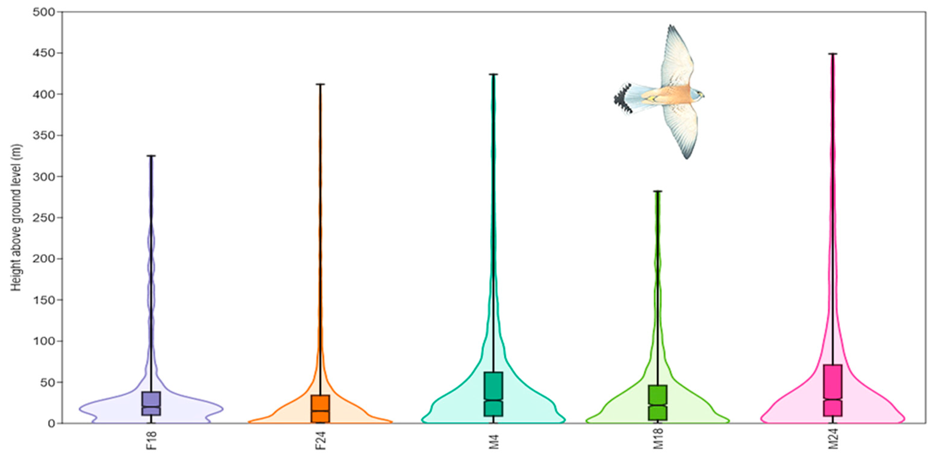
| F18 | 22.76 | 44 | 20 | 325 | 1.79 |
| F24 | 34.32 | 39 | 16 | 412 | 4.46 |
| M4 | 111.48 | 54 | 29 | 424 | 5.58 |
| M18 | 40.46 | 40 | 21 | 283 | 1.87 |
| M24 | 97.62 | 62 | 29 | 448 | 8.19 |
Disclaimer/Publisher’s Note: The statements, opinions and data contained in all publications are solely those of the individual author(s) and contributor(s) and not of MDPI and/or the editor(s). MDPI and/or the editor(s) disclaim responsibility for any injury to people or property resulting from any ideas, methods, instructions or products referred to in the content. |
© 2023 by the authors. Licensee MDPI, Basel, Switzerland. This article is an open access article distributed under the terms and conditions of the Creative Commons Attribution (CC BY) license (https://creativecommons.org/licenses/by/4.0/).
Share and Cite
Ferrarini, A.; Giglio, G.; Pellegrino, S.C.; Gustin, M. Overlap and Segregation among Multiple 3D Home Ranges: A Non-Pairwise Metric with Demonstrative Application to the Lesser Kestrel Falco naumanni. Biology 2023, 12, 77. https://doi.org/10.3390/biology12010077
Ferrarini A, Giglio G, Pellegrino SC, Gustin M. Overlap and Segregation among Multiple 3D Home Ranges: A Non-Pairwise Metric with Demonstrative Application to the Lesser Kestrel Falco naumanni. Biology. 2023; 12(1):77. https://doi.org/10.3390/biology12010077
Chicago/Turabian StyleFerrarini, Alessandro, Giuseppe Giglio, Stefania Caterina Pellegrino, and Marco Gustin. 2023. "Overlap and Segregation among Multiple 3D Home Ranges: A Non-Pairwise Metric with Demonstrative Application to the Lesser Kestrel Falco naumanni" Biology 12, no. 1: 77. https://doi.org/10.3390/biology12010077