Abstract
Diverse phenomena such as feedback, interconnectedness, causality, network dynamics, and complexity are all born from Relationships. They are fundamentally important, as they are transdisciplinary and synonymous with connections, links, edges, and interconnections. The foundation of systems thinking and systems themselves consists of four universals, one of which is action–reaction Relationships. They are also foundational to the consilience of knowledge. This publication gives a formal description of and predictions of action–reaction Relationships (R) or “R-rule”. There are seven original empirical studies presented in this paper. For these seven studies, experiments for the subjects were created on software (unless otherwise noted). The experiments had the subjects complete a task and/or answer a question. The samples are generalizable to a normal distribution of the US population and they vary for each study (ranging from N = 407 to N = 34,398). With high statistical significance the studies support the predictions made by DSRP Theory regarding action–reaction Relationships including its universality as an observable phenomenon in both nature (ontological complexity) and mind (cognitive complexity); mutual dependencies on other universals (i.e., Distinctions, Systems, and Perspectives); role in structural predictions; internal structures and dynamics; efficacy as a metacognitive skill. In conclusion, these data suggest the observable and empirical existence, parallelism (between cognitive and ontological complexity), universality, and efficacy of action–reaction Relationships (R).
1. Introduction
Typically, one provides a Methods, Introduction, Discussion, Results, and Conclusion for just one empirical study. However, for this publication, we keep all the different parts mentioned above, but we share seven studies rather than one. Publishing seven separate papers could only have benefited the authors. The decision was made to keep these seven studies together. They form a collection of studies that becomes an “ecology”. The rationale for the author’s decision is as follows. Four of seven studies were relatively small (usually a single question) testing a particular hypothesis and isolating a particular effect. Additionally, the studies focus on specific aspects of the same universal pattern (action–reaction Relationships rule) which means that the results can be understood better as a whole collection instead of isolated parts. We imagine that our reasoning makes sense to a journal focused on systems. That said, to read each study on its own, read Section 2.1, Section 3.1, and Section 4.1 together.
1.1. Empirical Findings of Relationships across the Disciplines
Drawing Relationships between and among entities is a concept that is explored across every discipline. The idea of Relationships has many names which includes synonyms and related terms such as: connect, relate, interconnection, interaction, link, cause, effect, affect, and rank; most words with the prefixes inter-, intra-, or extra- such as interdisciplinary, intramural; between, among, couple, associate, join; most words with the prefix co- as in correlate, cooperate or communicate; various types of Relationships such as linear, nonlinear, causal, feedback, linear causality, webs of causality, and even the basic mathematical operators such as +, −, /, and x. Any time we do any of the above, we are recognizing Relationships. That is, one idea or object is interrelating to another.
The ecology of seven studies discussed in this publication is contextualized in the large collection of literature of empirical studies and in existing literature reviews on Relationships. There is much interest in the scientific community, literature, research, and empirical findings on Relationships across the disciplines (i.e., the natural, physical, applied, and social sciences). The literature is well established on Relationships [1,2,3,4,5,6,7,8,9,10,11,12,13,14,15] in both the cognitive and systems thinking contexts. Relationships are fundamentally woven into the cognitive sciences (the physical and natural sciences as well) [4,8,9,12,14]. Causality, which is a part of the action–reaction Relationship rule, is present in adults and children [4,9,11,12,15], and can be utilized as, “(…) a tool for gaining deeper understanding [14]”. The definition of Relationships was expanded by Cabrera [16] by showing that: “(1) all relational processes were cases of Relationships between an action and a reaction variable and (2) that action-reaction Relationships were not reserved merely for ‘the systems’ cause and effects alone, but were structural features occurring on fractal dimensions [17].” This crucial understanding at the theoretical level, which is a subsection of DSRP Theory, brought to light that action–reaction Relationships are universal. This theoretical construct is empirically quantified by this study.
There are many empirical studies that clearly illustrate that action–reaction Relationships are universal across the disciplines [1,2,3,4,5,6,7,8,9,10,11,12,13,14,15,18], as shown in a 2021 review of literature by Cabrera [19]. However, Relationships are not enough. Relationships are critical but they are not sufficient enough to navigate real-world systems and their complexities or to explain an universal, underlying, and structural grammar of cognition. Action–reaction Relationships are integrated fundamentally with other universals (i.e., Distinctions, Systems, Perspectives), which DSRP Theory predicts [20,21,22,23,24,25,26,27,28,29,30,31,32,33,34,35,36,37,38,39,40,41,42,43,44,45,46,47,48,49,50,51]. These predictions are shown in empirical findings from the literature. Figure 1 shows the disciplinary distribution of this research.
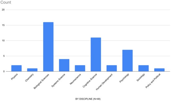
Figure 1.
Action–Reaction Relationships (R) Research Across the Disciplines.
The review of the research done by Cabrera in 2021 [19] builds upon two previous literature reviews [16,52]. It is, in a sense, a “tip of the iceberg”. The 2021 literature review [19] is part of a growing body of empirical research in support of action–reaction Relationships in particular, and DSRP theory predictions generally. The findings, utility, and application of action–reaction Relationships (R) are ubiquitous and pervasive. Some highlights from the literature review [19] are:
- Leonid Euler (1735) [18] solves the Konigsberg bridges problem and invents graph theory and modern day network theory based on identities (nodes) and Relationships (edges);
- Norbert Wiener (1948) [2] and John Weily (1951) [1] highlight a very important structural type of Relationship found within systems: feedback loops;
- Clement and Falmagne’s 1986 studies [3] of how comprehension increases with interconnectivity between content knowledge;
- Gopnik et al.’s 2004 study [4] on causal structures and the causal maps that children build to make sense of their world;
- Green’s 2010 study [6] showing that memory is a function of linking thoughts to one another;
- Ferry et al.’s 2015 research [9] showing that infants’ analogical ability is making “relational comparisons between objects, events, or ideas, and to think about relations independently of a particular set of arguments”.
1.2. Theoretical Work on Relationships
As Cabrera [17] writes, “The simplest accurate statement of DSRP Theory is thus”:

There is much more to DSRP Theory than this simplification relays [16,52,53,54,55]. Cabrera [17] remarks, “In addition, DSRP Theory has more empirical evidence supporting it than any existing systems theory (including frameworks, which are not theories) [16,17,19,56,57,58,59,60,61]. For more on DSRP Theory proper the reader should see the citations mentioned as this paper focuses solely on the “R” in DSRP: Relationships”.
As one of four DSRP universal Rules, action–reaction Relationships or the R-rule is applicable and effective across the disciplines from the social sciences to the physical and natural sciences. The transdisciplinary importance of action–reaction Relationships cannot be overstated. For example, the action–reaction Relationships (R) rule is at play in physics in Newton’s Third Law shown in Figure 2.
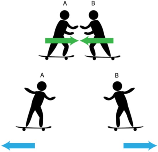
Figure 2.
Action–Reaction Relationships (R) Rule and Newton’s Third Law.
This same universal structure is characterized by the concept of a feedback loop, popularized by system dynamics, where one object or idea operates on another, which in turn operates on the first shown in Figure 3.
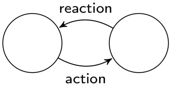
Figure 3.
Action–Reaction Relationships.
Additionally, this same universal structure is useful in psychosocial applications. Figure 4 illustrates how actions and reactions form a looping process in social dynamics. Being aware (metacognitive) of these social-dynamical structures and patterns allows an individual to process autonomic reactions (e.g., thoughts, feelings) internally and purposefully choose one’s action (outward behavior).
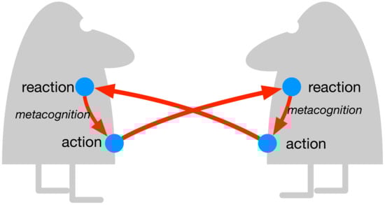
Figure 4.
Action–Reaction Relationships (R) Rule: “R quad” Used in PsychoSocial Applications.
This same relational structure provides the basis for “RDS’s” (Figure 5) which stands for Relationship-Distinction-System, helps us to see that when we make a Relationship between any two things or ideas, we will benefit greatly if we also (1) distinguish what that Relationship is by naming it and then, (2) systematize that Relationship by breaking it down into parts. RDSs are a powerful cognitive jig that allows us to see what is happening in Relationships and solve all kinds of problems from complex interpersonal social dynamics in a Relationship, to innovation, to solving the issue of silos in organizations.
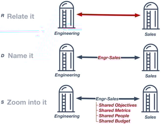
Figure 5.
RDSs is a Powerful Cognitive Jig that Reveals the Structure of Relationships.
The utility and application of action–reaction Relationships (R) are ubiquitous; there are countless more examples. Cabrera and Cabrera [16,19,52,62,63,64] expanded the transdisciplianry applicability of Relationships by detailing their internal dynamics and structures and identifying various mutual dependencies. Table 1 shows the structure of the action–reaction Relationships rule.

Table 1.
Action–Reaction Relationship Rule or R-rule.
It is quite popular in the Systems Sciences and Systems Thinking fields, and even in quantum physics [65,66], to propose that “it all comes down to Relationships”. At the same time that DSRP Theory predicts that action–reaction Relationships (R) are universal (as well as important and applicable), it is also predicted that Relationships are not enough [67]. Meaning that it all does not come down to Relationships because Relationships are dependent on other universals. Namely, Distinctions, Systems, and Perspectives. As Cabrera [17] writes, “DSRP theory comprises four dynamically interacting structures: identity-other Distinctions (D), part-whole Systems (S), action-reaction Relationships (R), and point-view Perspectives (P). Herein, we focus on point-view Perspectives (P). But, DSRP Theory also predicts that the four rules are dynamic and are necessary and sufficient. Thus, for a perspective to exist, the other rules need to be at play. Table 2 illustrates how Perspective itself, requires Distinctions, Systems, and Relationships to exist”.
Table 2.
DSRP is Necessary and Sufficient for R-rule [17].
1.3. Research Program That Underlies the Hypotheses for R-Rule Studies
Cabrera [16] expanded on Relationships theoretically by proposing in DSRP Theory that: (1) Relationships are universal to mind and nature (2) all Relationships (R) constitute an affect/effect Relationship between action (a) and reaction (r) variables (what Cabrera calls elements) and (3) that Relationships are not reserved merely connecting things but are things in and of themselves (what Cabrera calls identities). That is, any node in any network, or any element in an ecology, or any person, place, thing, or idea, has the potential to relate to others or be a Relationship between others and that these Relationships exist in nature (material systems) and can be taken by the human mind. Awareness of these existential Relationships (metacognition of R-rule) is crucial to increase one’s effectiveness in thinking about systems, modeling systems, or even in increasing cognitive fluidity, complexity, and robustness. Table 1 shows, according to DSRP theory, the structure of the action–reaction Relationships rule. Table 3 shows the basing for the hypotheses, null hypotheses, and research design and findings, which comprises the research matrix for this paper.
Table 3.
Research Program that Underlies the Hypotheses for R-rule Studies [17].
Thus, this set of studies on the R-rule of DSRP Theory is part of a research program that empirically tests the three major hypotheses represented in the matrix: Applied Research to establish the efficacy of DSRP in understanding Mind/Nature and Basic Research to establish the existence of DSRP in Mind/Nature. The following research questions were used on all four universal patterns [60]:
- 1.
- Existential (Basic Research): focused on the question: Does DSRP Exist? Does DSRP exist as a universal, material, observable phenomenon? [60]
- 2.
- Efficacy (Applied Research): focused on the question: Is DSRP Effective? Does metacognition of DSRP increase effectiveness in navigating cognitive complexity in order to understand system (ontological) complexity? This gets at the critically important question of “parallelism”—defined as the probability that our cognitive organizational rules align with nature’s organizational rules—which is central to the idea of the Systems Thinking/DSRP Loop [60] (Figure 6) (It should be noted that the ST/DSRP Loop is the mirror opposite of confirmation bias. Confirmation bias reverses this loop, by fitting reality to one’s mental models, whereas DSRP-Systems Thinking fits mental models to real-world observables and feedback. Parallelism is therefore the degree to which one’s cognitive paradigm, style, or mindset, aligns with nature’s. One purpose of this research program is to determine the degree to which DSRP Theory accomplishes this parallelism [60]).
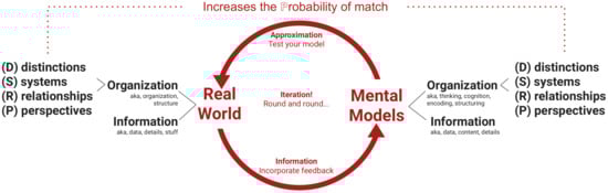 Figure 6. The ST/DSRP Loop.
This “ecology of empirical studies” includes multiple meta-analytical literature reviews [16,19] and 26 new empirical studies, as well as the 7 studies presented in this paper. For those who are interested in the other collections of studies, read the following: identity–other Distinctions (D) studies [60], point–view Perspectives (P) studies [59], and part–whole Systems (S) studies [61]. Thus, the empirical studies in this paper (each of which have separate hypotheses) address the following research program as an ecology of studies with respect to the R-rule:
- 1.
- Does the R-rule exist in Nature and Mind? (in the same way Evolution or Gravity exists)
- 2.
- Does metacognition (awareness) of the R-rule increase overall effectiveness in cognitive complexity or systems thinking or fluidity?
Although the design of the research studies focused on different aspects of this research program (again, each study has a separate hypothesis outlined in the study narrative), there is some overlap among these studies in their results and thus, together, they provide an ecological view of not only R-rule, but also its dependencies on D, S, and P rules. As a general guideline, however, one is safe to conclude that the Affective Squares, What Makes a Square, What Makes a Circle, and Dog–Lab–Coat studies were specifically focused on existential research questions and the R-Mapping Study, R-STMI Study (STMI is the acronym for the Systems Thinking and Metacognition Inventory), and R-Fishtank Study focused on efficacy. These studies, aim to demonstrate that the implications and theoretical predictions made by DSRP theory are empirically quantified in an observable and significant manner.
The concepts above were tested by each of the empirical research studies detailed in this paper. They each had their own hypotheses and had highly statistically significant results. We will now present the seven empirical studies that together form an ecology of findings.
2. Materials and Methods
The following information is true for all studies, unless otherwise noted. Subjects were asked to respond to a given task. Experiments were created using software for subjects to complete the tasks and/or answer questions. Several pilot tests were conducted prior to deployment to correct language-based confusion and to ensure construct validity. Sample size was chosen for generalizability (e.g., Given Confidence Level (CL = 95%), a US population estimated at 350,000,000, and Confidence Interval (CI = 5). The generalizable sample size was 384. Thus we chose sample sizes that were larger than this number). The samples themselves (range of N = 407 to 34,398 depending on the study) are generalizable to the United States population. Samples were created based on a normal distribution of the US population. Samples were identified using the following demographics, unless otherwise noted: 50/50 gender split; US population; between 22 and 65 years old; splits that were representative of the census numbers for education level (e.g., completion of high school, community college, college, masters, PhD). Samples, unless otherwise stated, were provided by Alchemer. Data were then analyzed and collected; note that nonsense data/incomplete data were removed from the analyzed data.
Details of the methods for each study are provided below.
2.1. The Affective Squares Study Methods
Statistical analysis was performed using R v 3.6.3. Counts and percentages were used to summarize the distribution of categorical variables. Bar plots were used to visualize the results. The Chi-square test for goodness of fit was used to assess whether the distribution of responses was not equal.
2.2. The What Makes a Square Study Methods
Statistical analysis for N = 406 was performed using R v 3.6.3. Counts and percentages were used to summarize the distribution of categorical variables. Bar plots were used to visualize the results. The Chi-square test for goodness of fit was used to assess whether the distribution of responses was not equal. Two-null hypotheses were tested in each trial. In addition, the responses between each pair of trials were compared using the Chi-square test of independence. Hypothesis testing was performed at a 5% level of significance.
2.3. The What Makes a Circle Study Methods
Statistical analysis for N = 406 was performed using R v 3.6.3. Counts and percentages were used to summarize the distribution of categorical variables. Bar plots were used to visualize the results. Chi-square test for goodness of fit was used to assess whether the distribution of responses was not equal. For each circle, hypotheses regarding size (small, medium, and big) and alignment (center, left, and right) were tested separately. Respondents who chose more than one size or alignment for each circle were excluded from the corresponding analysis. However, the frequency of answers chosen by the respondents was visualized. Hypothesis testing was performed at a 5% level of significance.
2.4. The Dog–Lab–Coat Study Methods
Statistical analysis was performed using R v 3.6.3. Counts and percentages were used to summarize the distribution of categorical variables. Bar plots were used to visualize the results. McNemar’s test was used to compare the distribution of responses before and after adding additional terms to the initial concept. Word clouds were used to visualize the responses. The use of various terms was compared before and after adding the additional term (dog or lab or coat). Hypothesis testing was performed at a 5% level of significance.
2.5. The R-Mapping Study Methods
This study utilized data from the software that was developed by Cabrera [68]: Plectica Systems Mapping Software. A self-selecting sample (N = 34,398) of software users was used in this study. The data were collected from a self-service web application that administers the Plectica software, including the limited demographic data that were collected. All four patterns of DSRP were included in the data collected. The results provided in this paper are for the Relationship pattern only. See [58] for a report of the wider data and context.
2.6. The R-STMI Study Methods
This study collected data from the Systems Thinking and Metacognition Indicator (STMI) which was developed by Cabrera and Cabrera [57]. The self-selecting sample (N = 1059) consisted of professionals between the ages of 18 and 65 who participated in the beta version of STMI after it was validated. Data were collected from the self-service web application that administers the STMI itself. Limited demographic data were collected as well. The data measures competence and confidence and cuts across all four patterns of DSRP and “mix and match of DSRP patterns”. The results provided in this paper are for the Relationship pattern only. See [57] for a report of the wider data.
2.7. The R-Fishtank Study Methods
The generalizable (see above in the general methods section) sample had a baseline section N = 1750 baseline and a post-treatment section N = 350. Data on all four patterns of DSRP were collected. The results provided in this publication are for the Relationship pattern only. See [58] for a report of the wider data.
3. Results
3.1. The Affective Squares Study Results
Subjects (N = 403) were asked to associate one of three shapes with one of three descriptions (Small, Medium, and Large Square). Table 4 shows the null and alternative hypotheses for this study.
Table 4.
Null and Alternative Hypotheses for Affective Squares Study.
The null hypothesis was , because if relational copriming effects do not exist, then one would expect that no difference would occur between the shape:name configurations; that is each of the three shapes had an equal probability of being named each of three labels. The alternative hypothesis was , because if relational copriming effects do exist, then one would expect to see significant differences to occur between the shape:name configurations; that is each of three shapes has an unequal probability of being named each of three labels. Table 5 shows that subjects overwhelmingly used a Relationships to distinguish the three shapes.
Table 5.
Affective Squares Study Results Shows the Relational Nature of Distinguishing Objects.
Table 6 shows statistical analyses for the responses and shows high statistical significance such that we can reject the null hypotheses. In other words, copriming effects based in Relationships do exist. Statistical analysis was performed using Chi-square G. Data were summarized using counts and percentages.
Table 6.
Statistical Analysis of Responses for Affective Squares Study.
Additionally, Figure 7 visually represents the overwhelming majority (97–99.5%) of respondents distinguished objects based on their Relationships to one another.
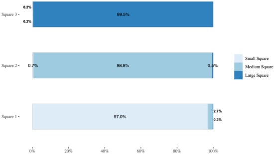
Figure 7.
Majority Distinguish Objects Based on Relationships.
3.2. The What Makes a Square? Study Results
In the first task of three, subjects (N = 406) were asked to identify a shape labeled “A” and given the following response choices: square, small square, medium square, and large square. Completion of the first task established a baseline because any answer could be “correct” given that the uncontextualized (no relational copriming) square could be considered a square or a small, medium, or large square. In the second and third tasks, the shape labeled “A” was put next to a copriming shape labeled “B” and in the third task two relational copriming shapes labeled “B” and “C”. Table 7 shows the alternative and null hypotheses for this study.
Table 7.
Hypotheses for What Makes a Square? Study.
Two null hypotheses— and —were tested, because if relational copriming effects do not exist, then one would expect no change to occur between the baseline and the second and third tasks (e.g., responses are completely independent of one another). The alternative hypothesis for Task 2 was , because if relational copriming effects do exist, then one would expect significant change (difference) to occur between the baseline and the second and third tasks (i.e., probability of answers are not equal). Likewise, the alternative hypothesis for Tasks 2 and 3 was .
In Task 1, subjects were asked to drag one of four responses to identify a shape labeled “A”. Table 8 shows that 55.17% (224/406) of subjects chose square. The remaining responses were spread across small square 3.69% (15/406), medium square 14.77% (60/406), and large square 26.35% (107/406).
Table 8.
Data for Tasks 1, 2, and 3—Relative Squares.
In Task 2, subjects were asked to identify a shape labeled “A” that was visually placed next to another smaller shape labeled “B”. The same answer choices were available: square, small square, medium square, and large square. In this case, large square was the chosen response at 75.36% (see Table 8), indicating the relational influence of the box “B” on the answer choice.
In Task 3, subjects (N = 406) were then asked to identify a shape labeled “A” that was placed between a smaller shape labeled “B” and a larger shape labeled “C”. The same choices were available: square, small square, medium square, and large square. In this case, 81.77% or 332/406 chose medium square (as shown in Table 8).
Table 9 shows the hypotheses-testing results for all three tasks. The null hypotheses are rejected for all three tasks with high statistical significance.
Table 9.
Hypothesis Testing Results for What Makes a Square? Study.
Table 10 shows the pairwise comparisons for the different tasks. Note that P-values were adjusted for pairwise comparisons, and we see highly statistically significant effects in each pair.
Table 10.
Pairwise Comparison of Tasks.
Additionally, Figure 8 visually represents the distribution of responses for each task object.
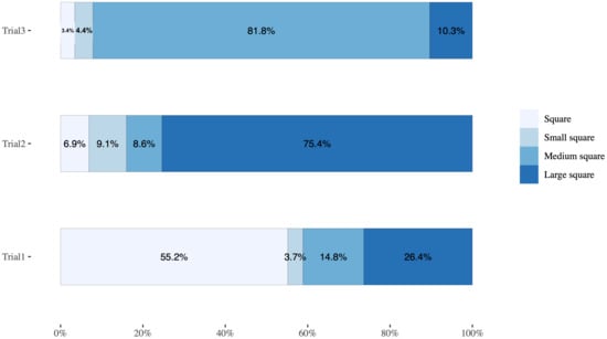
Figure 8.
Distribution of Responses.
Results showed that 55.2% chose “square” as a response to the first question. When another small square was added, three-quarters of the respondents chose “Large square”. When two additional squares were added (one smaller and one larger than the target square), 81.8% of the respondents chose “Medium square”.
3.3. The What Makes a Circle? Study Results
Subjects (N = 381) were shown three different sized circles presented from left (smallest) to right (largest) as shown in Figure 9. They were asked to identify whether each circle was: Left, Center, Right, Large, Medium, or Small and instructed to “select all that define each item”.

Figure 9.
The “What Makes a Circle?” Task.
We tested six null hypotheses (Table 11) (2 hypotheses × 3 circles). For each circle, two hypotheses were tested (one for size and one for alignment).
Table 11.
Hypotheses for What Makes a Square? Study.
Figure 10 shows results for all three circles in terms of size. Results showed that 85% of the respondents chose only one response for the size and 2–5% of the respondents chose 2 answers.
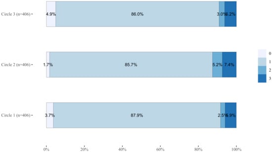
Figure 10.
Number of Size-Responses Chosen by Respondents for Each Circle.
Figure 11 shows results (for respondents who only chose 1 response) for all three circles in terms of size. Results showed that 96% of the respondents perceived circle 1 as small, circle 2 as medium, circle 3 as big.
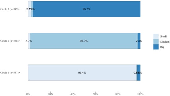
Figure 11.
Size of the Circle Chosen by Respondents (who chose 1 response).
Table 12 provides hypotheses-testing results for size choices for all three circles. The observed probability was significantly different from the expected equal probabilities (33%) under the null hypothesis for all three circles (p < 0.001 **).
Table 12.
Hypotheses testing for size.
Figure 12 shows the results for the relative alignment of circles (i.e., whether they are left, center, or right). Results showed that 30.5% chose two answers for circle 3. For circle 1, 83.5% chose 1 answer and 5.4% chose two answers. For circle 2, 10% chose two answers.
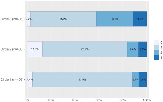
Figure 12.
Number of Responses Chosen by Respondents for Circle Alignment.
Table 13 shows detailed breakdowns of the various responses for Circle 3’s alignment. This detail was necessary due to the “anomalous” results for Circle 3. Of particular interest was that 37% who distinguished Circle 3 as being the “Center Circle”. A total of 124 respondents chose two answers for circle 3. Of these, 106 chose “center” and “right”.
Table 13.
Responses for circle 3 (analysis restricted to respondents who chose two answers).
Figure 13 shows that 97% of the respondents chose “left” for circle 1. Regarding circle 2, 25% of the respondents chose “left” and 67% chose “center” while 6.9% chose “right”. For circle 3, 10% chose “left” and “center”.
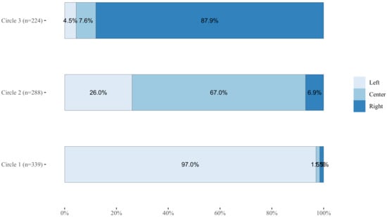
Figure 13.
Perceived alignment of the three circles (analysis was restricted to respondents who chose 1 answer).
Table 14 shows statistical analyses of hypotheses relative to alignment. Analysis was restricted to respondents who chose only 1 answer.
Table 14.
Hypotheses Testing for Alignment.
Results (Table 15 and Table 16) showed that the observed probabilities were significantly different from what was expected under the null hypothesis for all three circles (p < 0.001 **).
Table 15.
All respondents.
Table 16.
Respondents with only one choice.
3.4. The Dog–Lab–Coat Study Results
The null hypothesis was , because if relational copriming effects do not exist, then one would expect that no difference would occur between the first and second answer choice; that the probability that a description of X (i.e, each of the three terms: DOG, LAB, and COAT) changes when paired with another of these terms is 0. The alternative hypothesis was , because if relational copriming effects do exist, then one would expect that a difference would occur between the the first and second answer choice; that the probability that a description of X (i.e, each of the three terms: DOG, LAB, and COAT) changes when paired with another of these terms is >0.
Subjects (N = 366) (number of subjects varied by task) were asked a set of questions to determine the degree to which cognition relies on action–reaction Relationships among ideas or concepts. Subjects were first asked to describe in their words what they thought about when thinking about five things: Dog, Tree, Coat, Snow, and Lab. Tree and Snow were distractions used to ensure that Dog, Lab, and Coat in the baseline would not be affected. This technique was tested in prior research to verify its effectiveness. Subsequently, the data for Tree and Snow were deemed irrelevant to the study and are not provided herein.
Subjects’ unique results were cleaned by removing obvious misspellings and ignoring capitalization. For example, if a subject said “White Coat” and another said, “white coat” and another said “Wite caot” these three entries would be counted as one unique entry. Responses were open-ended, with no minimum or maximum length, and coded into similar terms. Descriptions provided by subjects for DOG were coded into 106 unique coded tags. LAB descriptions yielded 66 unique coded tags. Descriptions of COAT were coded into 39 unique tags. For coding/tagging purposes, answers that were obvious Nonsense, answers that provided a Literal response such as “the word coat”, and Other responses the meaning of which could not be determined, were removed from the analysis.
Counts for each unique coded tag were calculated and used to create a word cloud (Used R v3.6.3. and wordclouds.com (accessed on 1 Novemeber 2021)) for visual comparison to provide both a quantitative and qualitative view of the data to capture its richness. This provided a realistic picture of the meaning behind subject answers, shown in Table 17 for the baseline descriptions of DOG, COAT, and LAB. The combination of data and visual comparison makes the copriming effects of action–reaction Relationships quite stark.
Table 17.
Word Clouds of Un-Coprimed DOG, COAT, and LAB Baseline Concepts.
The data used to generate the word clouds are shown in Table 18, which shows that the “concepts” behind the descriptions of un-coprimed items are relatively typical. For example, a DOG (un-coprimed) is an animal with four legs including many breeds, some small, furry, barking, big, pets, cute, and white. A COAT is warm, for winter/cold, black or brown, clothing that can be worn and is comfortable. A LAB is a laboratory for science and experiments, used by scientists for chemistry with beakers, test tubes, etc.
Table 18.
Coded-tags for Un-Coprimed DOG, COAT, and LAB.
Once a baseline of concepts was established, subjects were then asked a set of four “coprimed questions” in which they were given two words from the three (DOG, LAB, COAT) in boxes and then asked to describe one of the words. We call this “copriming” because, provided at the same time, each word has a simultaneous priming effect on the other. Thus the hypothesis is that when copriming occurs, the conceptualization, meaning, and description of either one of the words will vary as a result of its copriming twin. For COAT–LAB coprimed COAT there were 24 coded tags. For DOG–LAB coprimed LAB there were 73 coded tags. For COAT–LAB coprimed LAB there were 75 coded tags. For DOG–COAT coprimed COAT, there were 55 coded tags. In addition, for each coprime study, a binary comparison was made using text analysis and coding by three researchers to determine if responses were, respectively, “COAT or DOG or LAB-like” (1) or not (0). These binary comparisons were used to determine the correlation coefficients, p-value, standard deviations, and averages.
3.4.1. Given COAT and LAB, Describe COAT
First, they were presented with the coprimed task: Given COAT and LAB, describe COAT. The word cloud in Table 19 visually illustrates what the data in Table 20 reveals: whereas subjects described a stereotypical “winter” or “warm” (34.88% of the time) and “black, brown or red” (9.8% of the time) COAT in the baseline measure, they were more likely to describe the COAT as “white or blue” (13.23%) and “labcoat”(28.40%) when the copriming took place.
Table 19.
Comparison of Un-Coprimed COAT to COAT–LAB coprimed COAT.
Table 20.
Coded-tags for COAT–LAB coprimed COAT.
From both the quantitative data and the visual word clouds one can see that when Subjects described only COAT, they predominantly described a jacket or winter-style coat. However, when coprimed with COAT and LAB together, they describe COAT as being both a winter, warm, jacket-style coat but a significant number of subjects also describe COAT as a white (or blue), scientists’ or doctors’ lab coat. This illustrates that the meaning of LAB has a LAB-like action on the meaning of COAT (and vice versa), thereby causing a significant number of subjects to describe the coat as a lab coat or include other scientific types of concepts.
In other words, the concept of LAB changed the concept of COAT (and likely vice versa). Instead of a warm winter coat, more subjects thought of a white lab coat. Some subjects’ responses included embodied stories that emerged just from the copriming. These include examples such as: “You take your coat off and go into the lab”; “The scientist had to put on his hazmat coat before entering the lab”; “It’s a coat made from a dog”; “The coat keeps you as warm as the dog”; These stories reinforce the cognitive tendency when given two or more objects or concepts, to identify the Relationship between them, even to go so far as to invent one where none exists.
A total of 203 respondents were included in the LAB–COAT study. McNemar’s test result was statistically significant, indicating a statistically significant change in responses before and after including the word LAB (shown in Table 21). Before including LAB, only one respondent used a lab-like answer compared to 202 who did not. Of the 202 who did not, 44.6% used lab-like answers after adding the word LAB to the original word COAT (p < 0.001 ***).
Table 21.
Comparison of terms before and after adding the word LAB to COAT.
Figure 14 compares the frequency of words used before and after. You can see that specifically, lab (as in “labcoat”) and white were more frequent descriptors of the COAT after whereas warm and black were more frequent before.
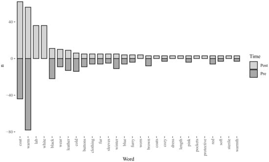
Figure 14.
Comparison of word frequency before and after adding the word LAB in the LAB–COAT task.
Figure 15 shows the difference in the frequency of words used before and after. Positive numbers indicate more frequent use after adding the word LAB, and negative numbers indicate more frequent use before adding LAB. For example, warm was used for the description of COAT 22 times more before and lab and coat were used to describe COAT 36 times more after.
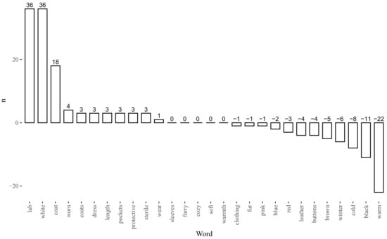
Figure 15.
The difference in the frequency of use of words before and after adding the word LAB.
The null hypothesis () that “Subjects answers show no lab-like change as a result of coprime” and an alternative Hypothesis () that “Participant answers show lab-like change as a result of the coprime” were tested. The unprimed COAT sample (N = 203) had 1 or 0.4% ‘lab-like’ responses. Whereas, the COAT–LAB coprime for the COAT sample (N = 203) had 90 or 44.6% ‘lab-like’ responses. We found a statistically highly significant Relationship between copriming and results. Thus, is rejected and is supported: “Participant answers show a lab-like change as a result of the coprime” indicating that action–reaction Relationships between objects and concepts exist. (The possibility of mediating variables in particular demographics of subjects was ruled out using contingency tables to cross tabulate the data by age, race, gender, ethnicity, and education level.)
3.4.2. Given DOG and LAB, Describe LAB
Second, subjects were presented with the following prompt: Given DOG and LAB, describe LAB.
In simple terms, the word cloud in Table 22 shows what the data in Table 23 reveal: when subjects described a stereotypical “scientists” (5.23%) or “science” (11.98%) “laboratory” (28.76%) for LAB in the baseline measure, they were significantly more likely to describe the LAB as “labrador” (17%) and “dog-in-a-laboratory,” (3.8%) or “veterinary lab” (3.5%) or “chocolate” when the copriming took place.
Table 22.
Comparison of Unprimed LAB to DOG–LAB coprimed LAB.
Table 23.
Coded-tags for Given DOG–LAB, Describe LAB.
In some cases, subjects created miniature stories such as “Where experiments are done on dogs”: ( or “Oh poor dog. Hopefully they aren’t doing tests on him” or “The veterinarian examined the dog in her lab,” or our favorite, “A science lab where the dog runs experiments”. In these cases, the interaction effects of DOG and LAB are obvious, and quite palpably different—both quantitatively and qualitatively—from the responses for DOG or LAB alone.
A total of 195 subjects were included in the DOG–LAB study. McNemar’s test result was statistically significant, indicating a statistically significant change in responses before and after including the word DOG (shown in Table 24). Before including DOG, fourteen respondents used dog-like answers compared to 181 who did not. Of the 181 who did not, 47% used dog-like answers after adding the word DOG to the original word “lab” (p < 0.001 ***).
Table 24.
Comparison of terms before and after adding the word DOG to LAB.
Figure 16 compares the frequency of words used before and after. One can see that dog and labrador were more frequent descriptors of the LAB after whereas science and experiments were more frequent before.
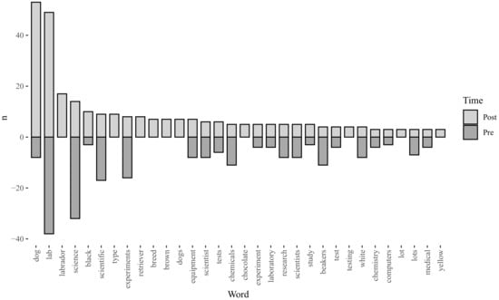
Figure 16.
Comparison of word frequency before and after adding the word DOG in the DOG–LAB task.
Figure 17 shows the difference in the frequency of words used before and after. Positive numbers indicate more frequent use after adding the word LAB, and negative numbers indicate more frequent use before adding DOG. For example, dog was used for the description of LAB 45 times more after and science and experiments were used to describe LAB 18 and 8 times more, respectively, before.
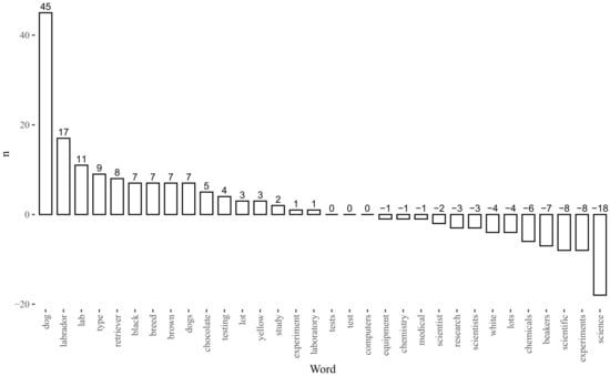
Figure 17.
The difference in the frequency of use of words before and after adding the word DOG.
The null hypothesis () that “Subjects answers show no dog-like change as a result of coprime” and an alternative Hypothesis () that “Participant answers show dog-like change as a result of the coprime” were tested. We found a highly statistically significant Relationship between copriming and affected results. Thus, is rejected and is supported: “Participant answers show dog-like change as a result of the coprime” or action–reaction Relationships between objects and concepts exist. (The possibility of mediating variables in particular demographics of subjects was ruled out using contingency tables to cross tabulate the data by age, race, gender, ethnicity, and education level.).
3.4.3. Given COAT and LAB, Describe LAB
Third, respondents were presented with: Given COAT and LAB, describe LAB.
In simple terms, the word cloud in Table 25 shows what the data in Table 26 reveals: when subjects described a stereotypical “scientists” (5.23%) or “science” (11.98%) “laboratory” (28.76%) for LAB in the baseline measure, they were significantly more likely to include “lab coat,” (11.9%), etc. in their description LAB when the copriming took place.
Table 25.
Comparison of Unprimed LAB to COAT–LAB Coprimed LAB.
Table 26.
Coded-tags for COAT–LAB Coprimed LAB.
A total of 202 respondents were included in the COAT–LAB study. McNemar’s test result was statistically significant, indicating a statistically significant change in responses before and after including the word COAT (shown in Table 27). Before including COAT, only seven respondents used coat-like answers compared to 195 who did not. Of the 195 who did not, 29.7% used coat-like answers after adding the word COAT to the original word “lab” (p < 0.001 ***).
Table 27.
Comparison of terms before and after adding the word COAT to LAB.
Figure 18 compares the frequency of words used before and after. One can see that coat and white were more frequent descriptors of LAB after whereas science and scientific were more frequent before.
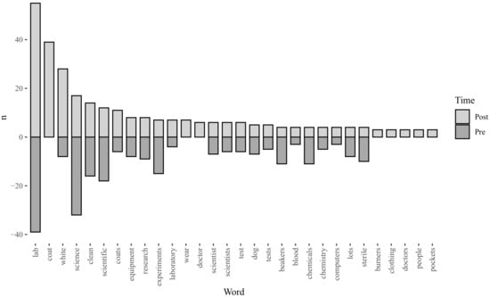
Figure 18.
Comparison of frequency of words used to describe LAB before and after for Given COAT–LAB, Describe LAB task.
Figure 19 shows the difference in the frequency of words used before and after. Positive numbers indicate more frequent use after adding the word COAT, and negative numbers indicate more frequent use before adding COAT. For example, coat was used for the description of LAB 39 times more after and science and experiments were used to describe LAB 15 and 8 times more, respectively, before.
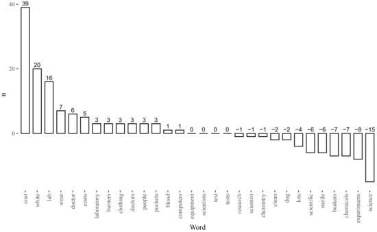
Figure 19.
The difference in the frequency of words used to describe LAB before and after for Given COAT–LAB, Describe LAB task.
The null hypothesis () that “Subjects show no coat-like change as a result of coprime” and an alternative Hypothesis () that “Subjects show coat-like change as a result of the coprime” were tested. We found a statistically highly significant Relationship between copriming and affected results. Thus, is rejected and is supported: “Participant answers show coat-like change as a result of the coprime” or action–reaction Relationships between objects and concepts exist.
3.4.4. Given DOG and COAT, Describe COAT
Fourth, respondents were presented with: Given DOG and COAT, describe COAT.
In simple terms, the word cloud Table 28 shows what the data in Table 29 reveals: where subjects described a stereotypical “winter” “warm” with “buttons” for COAT in the baseline measure, they were significantly more likely to describe the COAT as “fur” and “dog-clothing,” or “fluffy” when the copriming took place.
Table 28.
Comparison of Unprimed COAT to DOG–COAT Coprimed COAT.
Table 29.
Coded-Tags for DOG–COAT Coprimed COAT.
A total of 241 respondents were included in the DOG–COAT study. McNemar’s test result was statistically significant, indicating a statistically significant change in responses before and after including the word DOG (shown in Table 30). Before including DOG, only four respondents used dog-like answers compared to 237 who did not. Of the 237 who did not, 39.2% used dog-like answers after adding the word DOG to the original word COAT (p < 0.001 ***).
Table 30.
Comparison of terms before and after adding the word DOG to COAT.
Figure 20 compares the frequency of words used before and after. One can see that dog, fur, and coat were more frequent descriptors of COAT after whereas warm, cold, and leather were more frequent before.
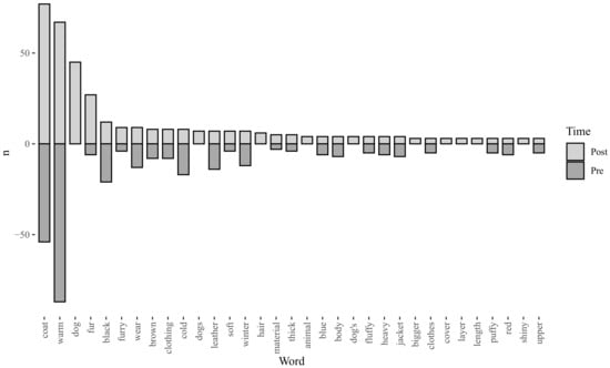
Figure 20.
Comparison of frequency of words used to describe COAT before and after for Given DOG–COAT, Describe COAT task.
Figure 21 shows the difference in frequency of words used before and after. Positive numbers indicate more frequent use after adding the word DOG, and negative numbers indicate more frequent use before adding DOG. For example, after the relational coprime, the description of COAT was 45 times more likely to include dog and 21 times for fur whereas before, COAT was described 20 times more as warm and 7 times more as leather.
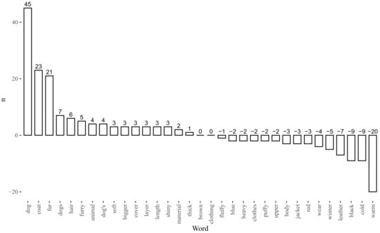
Figure 21.
The difference in the frequency of words used to describe COAT before and after for Given DOG–COAT, Describe COAT task.
The null hypothesis () that “Subjects show no coat-like change as a result of coprime” and an alternative Hypothesis () that “Subjects show coprime-like change as a result of the coprime” were tested across four tasks. We found a statistically highly significant Relationship (See Table 31) between copriming and affected results. Thus, is rejected and is supported: “Subjects answers show coprime-like change as a result of the coprime” or action–reaction Relationships between objects and concepts exist.
Table 31.
P-values for DOG–LAB–COAT Copriming.
3.5. The R-Mapping Study Results
To determine what people do and do not do when mapping a system, a study (n = 34,398) of aggregate data of software users in Plectica (Dr. Derek Cabrera invented Plectica Systems Mapping Software along with Dr. Laura Cabrera. It was used as a pilot software program for research for years. The Cabreras then co-founded Plectica to further develop the software for consumers. Plectica was then sold to Frameable, and Cabrera is no longer actively involved in the company) systems mapping software was performed. A total of 48% did nothing on their mapping canvas, which is consistent with research on people faced with an open-ended problem or question (mapping prompt) and/or a blank page or screen (mapping area). The research showed that the people had no response and took no action (i.e., they “froze”). However, 52% of people in the study made 2,066,654 identity distinctions. Further, 48% of people broke down their distinctions into 769,120 parts. A total of 46% of the people in the study made 565,999 Relationships between things. A total of 25% of people distinguished 87,318 Relationships by adding an identity (naming) to the relational line. This is also known as an “RDS” or a Relationship-Distinction-System. A total of 16% of people took at least one explicit perspective, with a total of 39,398 perspectives taken in the study. A total of 4% of people distinguished 16,668 perspectives in the software. A total of 2% of people included 3265 Relationships in the view of their perspective as shown in Table 32 [60].
Table 32.
Actions Users Take and Do Not Take When Systems Mapping (N = 34,398) [60].
The data from the R-Mapping Study provide insight into what people do when mapping, and what they do not do (or could have done but did not). Table 33 visually represents the difference between what people do (or did) and what they did not do (or could or should do). It provides a baseline for what systems thinkers should do more of and what they should continue to do.
Table 33.
What People Do and Do Not Do in Systems Mapping (N = 34,398) [60].
Less than half of people when given a blank canvas will make Relationships (we know that 46% of people related identities 565,999 times). Even further, only 25% of people distinguished their Relationships (87,318 times) or zoomed into them and added parts () or related the parts of the whole (). People rarely think in webs of causality (S of Rs), but they will look for the direct cause (R). As a metacognitive skill, Relationships, two jigs—”Part Parties” and “RDSs”, can be used to significantly increase cognitive complexity and efficacy in systems thinking, or even thinking as a whole.
3.6. The R STMI Study Results
In the STMI study [57] (N = 1059), subjects were shown to have exhibited the Dunning–Kruger Effect [69], where in the action–reaction Relationships (R) skill, confidence was higher than competence, as shown in Figure 22. This was the same across all four universals of DSRP Theory (action–reaction Relationships, part–whole Systems, point–view Perspectives, and identity–other Distinctions) but in this paper, we focus on the results for only the action–reaction Relationships skill. Subjects’ aggregate action–reaction Relationships confidence score was 85 while their competency/skill score was 72—a difference of 13.
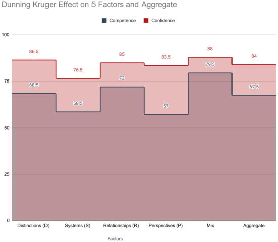
Figure 22.
Dunning–Kruger Effect in action–reaction Relationships [57].
3.7. The R-Fishtank Study Results
In the Fishtank Study [58], subjects (N = 1750) were asked to write out what they saw in a simple fishtank image (the image in Figure 23).

Figure 23.
Describe what you see [58].
The baseline data were established from the first round of responses. Then the subjects (N = 350) were given a > one-minute treatment that consisted of the bulleted text shown in Table 34.
Table 34.
Less than 1 Minute Treatment (M = 28.11 s) (from [58]).
Cabrera [58] explains, “Subjects were then shown the same fish tank image again and asked, “Describe what you see in the image when applying the action-reaction Relationships Rule you just learned (text copied below the image)”. This was called the Post-Relationships Treatment (or ‘PostR’). The results are shown qualitatively and visually: the differences between the word clouds generated for PreR and PostR are shown in Table 35.”
Table 35.
Word Clouds of PreR and PostR [58].
It is easy to see that the PostR word cloud is more descriptive and detailed than the PreR word cloud. Larger words mean more occurrences. Smaller words (which appear as grayish halo background) indicate more detail and more words used. We can see certain relational words—such as Relationship, and, to, and between—are prevalent in the PostR and nonexistent in PreR. PostR also has more terms (more tiny words producing a grey halo). We see these same patterns in the quantitative data. On every dimension, the PostR exceeded the PreR data (Table 36), indicating that PostR responses increased in their quantity and were more interrelational.
Table 36.
PreR and PostR Aggregate Response Data.
Relational words made up significantly more of the PostR total than in the PreR condition. Connector words like: and (78), in (67), of (61), to (61), Relationship (41), are (32), for (24), with (20), different (16), between (16) (see Table 37). In fact, relational words were 2.96 times more common, -ing words were 1.40 times more common, and verbs were 6.38 times more common in PostR than PreR (see Table 38).
Table 37.
PreR and PostR Top 40 Terms Used (from [58]).
Table 38.
PreR and PostR Relational Words Analysis of Unique Words.
Unique words and their occurrences were cleaned from the total words and the top 40 words from PreR and PostR are shown in Table 37.
Using median [IQR], the data (N = 382) was summarized. Using the Wilcoxon signed-rank test, statistical analysis was performed. The results in Table 39 demonstrate that the distribution of concepts was significantly different before and after treatment (p = <0.001 *** using Wilcoxon signed-rank test). After treatment, there were a lower average number of concepts observed. Cabrera [58] states, “The distribution of the number of words used after treatment (M = 4, IQR 2–9) was significantly different from that observed before treatment (M = 4, IQR 3–7, P = 0.003 *). The distribution of the number of characters used after treatment (M = 23, IQR 10–51) was significantly higher than the median number of words used before treatment (M = 23, IQR 13–38, P = 0.015 *).”
Table 39.
R comparison of raw counts, words, and characters before and after treatment (from [58]).
A less than one-minute treatment of the R-rule led the respondents to increase the complexity (with high statistical significance) of what they saw in a fish tank scene and how they described it. Figure 24 shows two of the many dimensions where the subjects increased the cognitive complexity of their responses with highly statistically significant results. Lewis and Frank [70] showed that conceptual complexity is reflected by the length of words.
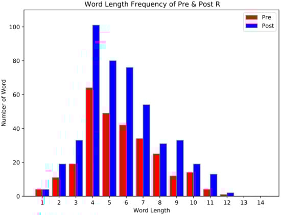
Figure 24.
Increased Cognitive Complexity of Response After Minute Treatment of R-Rule.
4. Discussion of Findings
In the Affective Squares Study, What Makes a Square, What Makes a Circle, and Dog–Lab–Coat studies, we see that the co-affecting effects of action–reaction Relationships (R) exist, and even if unconscious to the subject, occurs universally. We see too, that the act of distinguishing identities and others (D-rule), even in the most basic ideas and objects such as medium square, is dependent on R-rule and vice versa. We see that action–reaction Relationships exist in both mind and nature, as they can be easily deduced. All of these studies indicate that action–reaction Relationships (R), while universal, are also dependent on the other universals predicted by DSRP Theory (identity–other Distinctions (D), part–whole Systems (S), and point–view Perspectives (P)). Finally, the R-STMI, R-Mapping, and R-Fishtank studies illustrate the efficacy of R-rule as a metacognitive skill. Taken together as an ecology, these studies show the existence, universality, efficacy, and parallelism of action–reaction Relationships (R) with high statistical significance.
4.1. The Affective Squares Study Findings
Copriming effects, the result of Relationships, exist. People make Relationships without being asked to. Table 40 shows that the way people distinguish things is based on not only the essence of the thing itself but on how the thing relates to other things in its context. An overwhelming majority of the time (96.78%, 98.51%, and 99.26%) subjects dragged each label to the corresponding square relative to the other squares around it. Thus, meaning making is relational in nature, and objects or ideas have copriming effects (action–reaction) on each other. This shows that distinguishing any idea or object requires Relationships, often unconsciously, between and among other ideas and objects.
Table 40.
Relational Distinction Making of Objects (N = 403).
4.2. The What Makes a Square? Study Findings
The What Makes a Square? Study shows that the identity of something (in this case a square) is determined not only by what that something is (square) but also by what it is not (small, medium, large) in relation to other things (in this case, other squares). It shows that when two items exist in the same “domain of discourse” there is a copriming effect where one object acts upon and reacts to the other and vice versa. The results of this study also show the relational nature of distinction-making and demonstrate that making Relationships is empirical. “A” is distinguished not merely based on what it is (a square) but also in relation to the other objects it is with (larger or smaller squares).
The dynamism of relational copriming was tested to see if the same identity changed when the other objects around it (its context) changed. In other words, in Table 41 the identity of square A changes when its position or relation to other squares changes. In the baseline condition the majority of subjects, when asked to identify square A, chose “square” (55.17%); other answer choices were equally plausible given that the square had no context in terms of size. In the second task, subjects were asked again to identify square-A and 75.36% selected Large Square. In the third task, square A was larger than B but smaller than C and 81.77% chose Medium Square. The findings for the What Makes a Square Study is that squares are relative. That is, whenever something appears or exists in the same domain as something else (which barring a vacuum is always, and even a vacuum is something other than the thing) those items, objects, and ideas are copriming. They are relative. Square A is neither inherently large nor inherently small nor inherently medium. It is small relative to larger squares, and large relative to smaller squares. The same could be said for any attributes. A square is relatively more squary than a circle which is relatively more circly than a square. Colors are brighter or darker relative to the other colors they are with. Our roles change, and even our personality and demeanor, relative to whom we are around. A newborn son brings a father into existence at the same time that the father makes the son exist. These dynamical changes are relative.
Table 41.
Relative Square Data (N = 406).
This study shows that distinguishing the same object as given in three independent tasks, shows that for each task a new distinction was made, independent of the prior task. This independence was caused by the (often unconscious) Relationship between objects. Normally, priming effects would occur as a result of previous tasks (cross-task), but in this case, we see that the priming occurs relationally within each task. In other words, regardless of the prior task, subjects made new distinctions based on object A’s Relationships to the other objects offered in the task. Importantly, this shows that a Relationship (even a subconscious one) acts as a perspective and is necessary for distinction-making.
4.3. The What Makes a Circle? Study Findings
The What Makes a Circle? study further illustrates the relative, or relational, nature of distinction making that was shown in the What Makes a Square? study. In other words, in both studies, a square/circle is distinguished not merely based on what it is (a square/circle) but also relative to the other objects it is with (larger or smaller squares/circles and left, middle, or right circles).
Of note, while it is clear that subjects distinguished each circle relationally, it also appears that in the case of the middle circle 29.92% of subjects labeled it as “left” indicating that they switched perspective midstream and considered the middle circle to be to the left of the right circle (only 8.66% did so in reverse for right of the left circle). In other words, each response is based on a Relationship to the other circles, and even when the physical position is not as clear as in the center circle, the responses given were still based on a Relationship between the center circle and either the circle to its right or left side.
We agonized over the apparent anomaly in the data (see Table 13). Why would such a large number of respondents distinguish Circle 3 as being the “Center Circle?” All of the other data made sense and supported the Alternative Hypotheses with high statistical significance, even with this anomaly. However, it was still a mystery to us. We kept asking, “How could 37% of respondent answers distinguish the far-right, large circle as being center?” We checked and quadruple checked the data. Then we looked at the actual screen that respondents were looking at when they did the task shown in Figure 25. Circle 3 was actually positioned in the center of the screen!

Figure 25.
Circle 3 Center?
In fact, as Table 42 shows subjects overwhelmingly did what was expected by the alternative hypothesis but they also did some less expected things (shown as implicit expected (↔) and unexpected (↔) Relationships). One can see that in each answer chosen, the subject altered the Relationships they were considering and not considering. However, they also redrew the boundaries of the Systems (shown as []) leaving some circles in and out (Distinctions) out of consideration (shown in (gray). In addition, with each defining answer, subjects recast their Perspectives (shown as =by size; = by position). What this means is that even in a simple task such as defining three circles by six descriptors, at each decision point subjects are dynamically recasting the D, S, R, and P structures to make meaning and arrive at conclusions.
Table 42.
Implicit expected (↔) and unexpected (↔) Relationships, Systems ([]), Perspectives (=by size; = by position), and Distinctions (gray) used in defining a circle.
There is a perspective (represented by brackets [ ]) which is provided by the researchers of the initial question. This perspective is comprised of the three circles such that. Subjects therefore decide whether Circle 2 is Center or Medium based on Relationships between the circles within this context . Remarkably, what we see is that, while subjects use this perspective the majority of the time, they also alter the perspective to yield different but equally plausible responses. For example, Circle 2 is left of Circle 3 but in order for this to be the case, Circle 1 must be ignored, or left out of the perspective such that (note also the part–whole systematization). In this case, Circle 2 is "to the left" of Circle 3. In Table 42 we see the expected (Alternative Hypotheses) Relationships denoted by ↔, but we also see a significant number of reframed perspectival and relationaldistinctions denoted by [↔]. While this study intended to show the influence of co-Relationships on distinction making, subjects showed us the natural influence of perspective on distinction making yielding unexpected but completely rational responses about the Relationships among the circles. Indeed, as Figure 25 shows, subjects not only created new perspectives inside the one given to them by researchers but also created new perspectives well-outside of the bounds of the research. This illustrates the fractal nature of Perspectives, Relationships, Systems, Distinctions, and DSRP.
4.4. The Copriming Dog–Lab–Coat Study Findings
The results of this study clearly show that (1) action–reaction Relationships (R) exist and also that any two words that appear in the same domain will have copriming effects as a result of the R rule. Indeed, it is because of the R rule that priming effects work as a research technique. It is also why savvy marketing campaigns informed by neuromarketing are able to repeatedly place two or more items in proximity (e.g., Coke/Life, Happy/Meal, Osama/Obama) and manipulate consumers for votes, money, or attention.
The highly statistically significant results of this study, combined with results from the other studies, show that just like fireflies and other organisms in nature can be mutually reinforcing (excitatory or inhibitory) coupled oscillators that influence the emergent properties of system-wide behavior [71,72] concepts too, can be coupled oscillators. This has important implications and applications for DSRP Theory because it confirms several of the hypotheses, implications, and predictions that DSRP Theory makes.
First, action–reaction Relationships (R) are central to the co-implication rule between the two elements of each of the four patterns (identity–other Distinctions (D), part–whole Systems (S), action–reaction Relationships (R), and point–view Perspectives (P)).
Second, action–reaction Relationships (R) are instrumental to the simultaneity dynamics in structural predictions. The massively relational nature of fireflies and other organisms in complex adaptive systems mimic those of concepts (DOG, LAB, COAT) when they exist in proximity to each other. They form an copriming network where n number of nodes in the network are copriming with the other nodes in the network. Likewise all eight elements of DSRP act simultaneously as the other seven and—acting as coupled oscillators—”vibrate” each other into existence. Vibrate may seem like a strange word to use here, but it captures the essence of these affecting–effecting action–reaction Relationships (see Figure 26). Indeed, any pair or collection of things, in both mind and nature (e.g., words, concepts, organisms, objects) can exhibit these kinds of action–reaction Relationships.
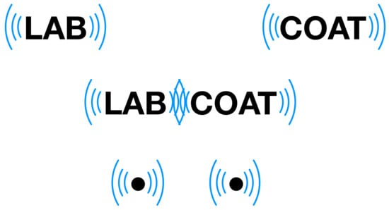
Figure 26.
R-rule and Domain Proximity.
In other words, action–reaction Relationships are as prevalent in DSRP Theory as they are among any things in reality (words, organizations, and people).
Third, these copriming effects (as a simple rule between any agents in any system) mean that any parts of a whole, by their proximity in sharing the same containment, have a high probability of interrelationship, thus the structural prediction based on these properties is highly probabilistic.
Fourth, the findings of these studies clarify important disagreements about order of operations between any two items; as it shows that it is so often the case that “both occur in unison”. Thus, in DSRP Theory, in the same way that a man becomes a father at the very moment when a boy becomes a son, it is also the case that a Perspective forms as the oscillation of point–view; a System forms on the coupling of part and whole; a Distinction is born as twin-births of identity and other.
Fifth, it means that even a relatively innocuous addition to a system of parts can have a transforming effect on the whole. This is precisely because of the action–reaction Relationships that occur when parts are in proximity.
4.5. The R-Mapping Study Findings
The studies previously discussed explore the fundamental existence of action–reaction Relationships. The STMI, Fishtank, and the R Mapping data show that action–reaction Relationships exist in Mind and Nature. Amazingly, the data also show that action–reaction Relationships, with a highly statistically significant effect, are able to be used metacognitively. This skill is able to be measured in terms of confidence and competence.
As shown in Table 32, subjects “freeze” when faced with a blank canvas, in fact, 48% did not do anything. This is because people become overwhelmed by the potential options when asked open-ended questions or when they are allowed to do “anything”. This finding matches with research and anecdotal experience. A total of 52% of the subjects did something. First off, they created a “thing” or an identity. This behavior is indicative of a Distinction. If you look at Table 32, it gives greater detail on what the sample (n = 34,398) did and did not do in this study. The statistics teach us much about metacognition. A summary of the data and what can be learned from it is provided in Table 33. The table shows a list of things you can keep doing and things you can work to do more of to improve your cognitive complexity and metacognitive skills. This is a best practices list for systems thinking, cognitive complexity, and metacognition. Doing more of the items on this list and being aware of them is systems thinking.
4.6. The R-STMI Study Findings
Action–reaction Relationships, as a universal, can be measured in both competence/skill and confidence. Action–reaction Relationships is a metacognitive skill as shown in both the Fishtank Study and the R STMI Study (both the Fishtank and the STMI Study focused on more than just the existence of action–reaction Relationships, see [57]). Additionally, the Dunning–Kruger effect is shown in our sample. The presence of the Dunning–Kruger effect shows that one should be careful not to overestimate our competency in the action–reaction Relationships skill.
4.7. The R-Fishtank Study Findings
The R-Fishtank Study shows that a less than 1 min treatment on the key concepts of action–reaction Relationships has a positive effect (with high statistical significance) on cognitive complexity. After the treatment, subjects saw qualitatively more and quantitatively deeper. Given the minimal time exposed to treatment (on average, a 28.11 s read), the findings indicate a highly statistically significant increase in the degree to which people made more detailed perspectives. With a different treatment (such as a longer online course) the effects could be truly transformative.
4.8. Summary of Findings on Existence, Universality, Efficacy, and Parallelism
In these seven studies, we see that the action and reaction elements of the Relationships pattern are inextricably linked, co-implying and interchangeable.
In Equation (1) we see that if in the domain of discourse () there exists (∃) any content information A and B, then A will have an A-like action () on B and vice versa. Additionally, B will have an B-like reaction () on A and vice versa. Thus, if an action (∃), then it implies (⇒) that a reaction exists and vice versa. Thus, action and reaction, as structural patterns of cognition are co-implying.
Thus, in Equation (2), we see that the action–reaction elements of Relationships are universal to all forms of links, causes, connections, edges, etc. Additionally, these universal elements are interchangeable such that any action can also function as reaction and vice versa:
In the other collections of studies, the part and whole variables of Systems (S) [61], the identity and other variables of Distinctions (D) [60], and the point and view variables of Perspectives (P) [59], were all shown to be action–reaction Relationships (R), for example, that the elements of D, S, and P are all copriming and co-implying. Like the studies presented herein for action–reaction Relationships (R), an ecology of studies was undertaken to test the existence and efficacy of, respectively, D, S, and P rules. These studies show that R is a factor in the formation of identity–other Distinctions, part–whole Systems, and point–view Perspectives.
These seven studies (along with the other studies mentioned) provide an “ecology” of findings about action–reaction Relationships. Each study adds a brick to the wall of our understanding of action–reaction Relationships (a.k.a., links, causes, connections, edges) and answers important questions about: (1) the role they play in metacognition, (2) the role they play in individual and social cognition, (3) their internal and external dynamics, (4) how and why they form, and (5) the effects of metacognitive awareness of action–reaction Relationships on overall cognitive complexity.
The What Makes a Square? and What Makes a Circle? studies illustrate the relative, or relational, nature of distinction making: that a square is distinguished not merely based on what it is (a square) but also relative to the other objects it is with (larger or smaller squares). Combined with previous Distinction studies, these relational, identity–other studies elucidate how the multiplicity of names (distinctions) that any given item can have, creates an “other-like” network of relations that, while often unconscious, is essential to the way that associative cognition operates. The Affective Squares study buttresses these findings and extends them to show that meaning making is relational in nature and objects or ideas have universal relational copriming effects (action–reaction) on each other. The Copriming Dog–Lab–Coat study explicates (to high statistical significance) these relational copriming (action–reaction) effects between concepts and objects and shows the universality of Relationships to cognition.
From the results of these seven studies of action–reaction Relationship structure detailed above, we can conclude that action–reaction Relationships (R) are:
- 1.
- Universal to the organization of Information:
- (a)
- in the mind (i.e., thinking, metacognition, encoding, knowledge formation, science, including both individual and social cognition);
- (b)
- in nature (i.e., physical/material, observable systems, matter, scientific findings across the disciplines);
- (c)
- because both mind and nature are material, distinct material identities and part–whole Systems (e.g., RDSs);
- (d)
- the basis for massively parallel action–reaction effects in networks in both mind and nature (i.e., action–reaction Relationships (R) form an copriming network where n number of nodes in the network are copriming with the other nodes in the network).
- 2.
- Made up of elements (action, reaction) that are:
- (a)
- co-implying (i.e., if one exists, the other exists; called the co-implication rule);
- (b)
- related by a special (“Special” here refers to the specific Relationship. In contrast to general or universal Relationships) Relationship: effect/affect;
- (c)
- act simultaneously as, and are therefore interchangeable with, the elements of Distinctions (identity, other), Systems (part, whole), and Perspectives (point, view). This is called the simultaneity rule.
- 3.
- Mutually dependent on identity–other Distinctions (D), part–whole Systems (S), point–view Perspectives (P) such that D, S, R, and P are both necessary and sufficient;
- 4.
- Taken metacognitively:
- (a)
- constitute the basis for making structural predictions about information (based on co-implication and simultaneity rules) of observable phenomena and are therefore a source of creativity, discovery, innovation, invention, and knowledge discovery;
- (b)
- effective in navigating cognitive complexity to align with ontological systems complexity.
To summarize what was found, we can return to our table of research questions (Table 3). In conclusion, these data suggest the empirical and observable universality, efficacy, existence, and parallelism (between cognitive and ontological complexity) of action–reaction Relationships (R) and with high statistical significance point to the conclusions and summaries in Table 43.
Table 43.
Summary Table of Conclusions.
Author Contributions
All Authors contributed equally in methodology, software, validation, formal analysis, investigation, resources, data curation, writing—original draft preparation, writing—review and editing, visualization, supervision, project administration, and funding acquisition. Development of DSRP Theory, D.C. All authors have read and agreed to the published version of the manuscript.
Funding
This research received no external funding.
Institutional Review Board Statement
Ethical review and approval were waived for this study due to no collection of personal or identifying data.
Informed Consent Statement
Informed consent was obtained from all subjects involved in the study.
Data Availability Statement
The data presented in this study are available on request from the corresponding author. The data are not publicly available due to privacy, human subjects, and ethical considerations.
Conflicts of Interest
The authors declare no conflict of interest.
Abbreviations
The following abbreviations are used in this manuscript:
| DSRP | DSRP Theory (Distinctions, Systems, Relationships, Perspectives) |
| D | identity–other Distinctions |
| S | part–whole Systems |
| R | action–reaction Relationships |
| P | point–view Perspectives |
| STMI | Systems Thinking and Metacognition Inventory |
| IQR | Interquartile range |
| GLMM | Generalized linear mixed modeling |
| RDS | Relate–Distinguish–Systematize Jig |
References
- Weily, J. Review of Cybernetics or Control and Communication in the Animal and the Machine. Psychol Bull. 1949, 46, 236–237. [Google Scholar] [CrossRef]
- Wiener, N. Cybernetics or Control and Communication in the Animal and the Machine; MIT Press: Cambridge, MA, USA, 1961. [Google Scholar]
- Clement, C.A.; Falmagne, R.J. Logical reasoning, world knowledge, and mental imagery: Interconnections in cognitive processes. Mem. Cogn. 1986, 14, 299–307. [Google Scholar] [CrossRef] [PubMed]
- Gopnik, A.; Glymour, C.; Sobel, D.M.; Schulz, L.E.; Kushnir, T.; Danks, D. A theory of causal learning in children: Causal maps and Bayes nets. Psychol. Rev. 2004, 111, 3–32. [Google Scholar] [CrossRef] [PubMed]
- Schulz, L.E.; Gopnik, A. Causal learning across domains. Dev. Psychol. 2004, 40, 162–176. [Google Scholar] [CrossRef]
- Greene, A.J. Making Connections. Sci. Am. Mind 2010, 21, 22–29. [Google Scholar] [CrossRef]
- Piao, Y.; Yao, G.; Jiang, H.; Huang, S.; Huang, F.; Tang, Y.; Liu, Y.; Chen, Q. Do pit vipers assess their venom? Defensive tactics of Deinagkistrodon acutus shift with changed venom reserve. Toxicon 2021, 199, 101–108. [Google Scholar] [CrossRef]
- Chersi, F.; Ferro, M.; Pezzulo, G.; Pirrelli, V. Topological self-organization and prediction learning support both action and lexical chains in the brain. Top. Cogn. Sci. 2014, 6, 476–491. [Google Scholar] [CrossRef]
- Ferry, A.L.; Hespos, S.J.; Gentner, D. Prelinguistic Relational Concepts: Investigating Analogical Processing in Infants. Child Dev. 2015, 86, 1386–1405. [Google Scholar] [CrossRef]
- Kominsky, J.F.; Strickland, B.; Wertz, A.E.; Elsner, C.; Wynn, K.; Keil, F.C. Categories and Constraints in Causal Perception. Psychol. Sci. 2017, 28, 1649–1662. [Google Scholar] [CrossRef]
- Harris, P.L.; German, T.; Mills, P. Children’s use of counterfactual thinking in causal reasoning. Cognition 1996, 61, 233–259. [Google Scholar] [CrossRef]
- Mascalzoni, E.; Regolin, L.; Vallortigara, G.; Simion, F. The cradle of causal reasoning: Newborns’ preference for physical causality. Dev. Sci. 2013, 16, 327–335. [Google Scholar] [CrossRef]
- Rolfs, M.; Dambacher, M.; Cavanagh, P. Visual adaptation of the perception of causality. Curr. Biol. 2013, 23, 250–254. [Google Scholar] [CrossRef]
- Dhamala, M. What is the nature of causality in the brain?—Inherently probabilistic: Comment on “Foundational perspectives on causality in large-scale brain networks” by M. Mannino and S.L. Bressler. Phys. Life Rev. 2015, 15, 139–140. [Google Scholar] [CrossRef]
- Sanefuji, W.; Haryu, E. Preschoolers’ Development of Theory of Mind: The Contribution of Understanding Psychological Causality in Stories. Front. Psychol. 2018, 9, 955. [Google Scholar] [CrossRef]
- Cabrera, D. Systems Thinking; Cornell University: Ithaca, NY, USA, 2006. [Google Scholar]
- Cabrera, D.; Cabrera, L. DSRP Theory: A Primer. Systems 2022, 10, 26. [Google Scholar] [CrossRef]
- Euler, L. Solutio problematis ad geometriam situs pertinentis. Commentarii academiae scientiarum Petropolitanae. 1736, 6, 128–140. [Google Scholar]
- Cabrera, D.; Cabrera, L.; Cabrera, E. A Literature Review of the Universal Patterns and Atomic Elements of Complex Cognition. In Routledge Handbook of Systems Thinking; Cabrera, D., Cabrera, L., Midgley, G., Eds.; Routledge: London, UK, 2021. [Google Scholar]
- Bateson, G. Form Substance and Difference; Institute of General Semantics: New York, NY, USA, 1970. [Google Scholar]
- Von Bertalanffy, L. The history and status of general systems theory. Acad. Manag. J. 1972, 15, 407–426. [Google Scholar]
- Rittel, H.W.J.; Webber, M.M. Dilemmas in a general theory of planning. Policy Sci. 1973, 4, 155–169. [Google Scholar] [CrossRef]
- Marchal, J.H. On the Concept of a System. Philos. Sci. 1975, 42, 448–468. [Google Scholar] [CrossRef]
- Goguen, J.A.; Varela, F.J. Systems And Distinctions: Duality And Complementarity. Int. J. Gen. Syst. 1979, 5, 31–43. [Google Scholar] [CrossRef]
- Ivan, M.; Kondo, K.; Yang, H.; Kim, W.; Valiando, J.; Ohh, M.; Salic, A.; Asara, J.M.; Lane, W.S.; Kaelin, W.G., Jr. HIFa Targeted for VHL-Mediated Destruction by Proline Hydroxylation: Implications for O Sensing. Science 2001, 292, 464–468. [Google Scholar] [CrossRef] [PubMed]
- Chen, P.; Fan, D.; Zhang, Y.; Selloni, A.; Carter, E.A.; Arnold, C.B.; Dankworth, D.C.; Rucker, S.P.; Chelikowsky, J.R.; Yao, N. Breaking a dative bond with mechanical forces. Nat. Commun. 2021, 12, 5635. [Google Scholar] [CrossRef] [PubMed]
- Wadhams, G.H.; Armitage, J.P. Making sense of it all: Bacterial chemotaxis. Nat. Rev. Mol. Cell Biol. 2004, 5, 1024–1037. [Google Scholar] [CrossRef] [PubMed]
- Janetopoulos, C.; Firtel, R.A. Directional sensing during chemotaxis. FEBS Lett. 2008, 582, 2075–2085. [Google Scholar] [CrossRef]
- Ikeya, N.; Woodward, J.R. Cellular autofluorescence is magnetic field sensitive. Proc. Natl. Acad. Sci. USA 2021, 118, e2018043118. [Google Scholar] [CrossRef]
- Förster, D.; Helmbrecht, T.O.; Mearns, D.S.; Jordan, L.; Mokayes, N.; Baier, H. Retinotectal circuitry of larval zebrafish is adapted to detection and pursuit of prey. eLife 2020, 9, e58596. [Google Scholar] [CrossRef]
- De Corte, B.J.; Navarro, V.M.; Wasserman, E.A. Non-cortical magnitude coding of space and time by pigeons. Curr. Biol. 2017, 27, R1264–R1265. [Google Scholar] [CrossRef]
- Schnell, A.K.; Loconsole, M.; Garcia-Pelegrin, E.; Wilkins, C.; Clayton, N.S. Jays are sensitive to cognitive illusions. R. Soc. Open Sci. 2021, 8, 202358. [Google Scholar] [CrossRef]
- Giannoni-Guzmán, M.A.; Rivera, E.; Aleman-Rios, J.; Melendez Moreno, A.M.; Ramos, M.P.; Pérez-Claudio, E.; Loubriel, D.; Moore, D.; Giray, T.; Agosto-Rivera, J.L. The Role of Colony Temperature in the Entrainment of Circadian Rhythms of Honey Bee Foragers. Ann. Entomol. Soc. Am. 2021, 114, 596–605. [Google Scholar] [CrossRef]
- Mareschal, D.; Quinn, P.C. Categorization in infancy. Trends Cogn. Sci. 2001, 5, 443–450. [Google Scholar] [CrossRef]
- Ashby, F.G.; Ell, S.W.; Waldron, E.M. Procedural learning in perceptual categorization. Mem. Cogn. 2003, 31, 1114–1125. [Google Scholar] [CrossRef]
- Sloutsky, V.M. The role of similarity in the development of categorization. Trends Cogn. Sci. 2003, 7, 246–251. [Google Scholar] [CrossRef]
- Lewis, M.; Balamurugan, A.; Zheng, B.; Lupyan, G. Characterizing Variability in Shared Meaning through Millions of Sketches. In Proceedings of the Annual Meeting of the Cognitive Science Society, Vienna, Austria, 3 February 2021. [Google Scholar]
- Lewandowsky, S.; Roberts, L.; Yang, L.X. Knowledge partitioning in categorization: Boundary conditions. Mem. Cogn. 2006, 34, 1676–1688. [Google Scholar] [CrossRef][Green Version]
- Sperry, R.W. Cerebral Organization and Behavior: The split brain behaves in many respects like two separate brains, providing new research possibilities. Science 1961, 133, 1749–1757. [Google Scholar] [CrossRef]
- Lupyan, G. The conceptual grouping effect: Categories matter (and named categories matter more). Cognition 2008, 108, 566–577. [Google Scholar] [CrossRef]
- Van Dijk, J.; Kerkhofs, R.; van Rooij, I.; Haselager, P. Special Section: Can There Be Such a Thing as Embodied Embedded Cognitive Neuroscience? Theory Psychol. 2008, 18, 297–316. [Google Scholar] [CrossRef]
- Mahon, B.Z.; Caramazza, A. Concepts and categories: A cognitive neuropsychological perspective. Annu. Rev. Psychol. 2009, 60, 27–51. [Google Scholar] [CrossRef]
- Cira, N.J.; Benusiglio, A.; Prakash, M. Vapour-mediated sensing and motility in two-component droplets. Nature 2015, 519, 446–450. [Google Scholar] [CrossRef]
- Tweedy, L.; Thomason, P.A.; Paschke, P.I.; Martin, K.; Machesky, L.M.; Zagnoni, M.; Insall, R.H. Seeing around corners: Cells solve mazes and respond at a distance using attractant breakdown. Science 2020, 369, eaay9792. [Google Scholar] [CrossRef]
- Blackiston, D.; Lederer, E.; Kriegman, S.; Garnier, S.; Bongard, J.; Levin, M. A cellular platform for the development of synthetic living machines. Sci. Robot. 2021, 6, eabf1571. [Google Scholar] [CrossRef]
- Tarrant, M.; Calitri, R.; Weston, D. Social identification structures the effects of perspective taking. Psychol. Sci. 2012, 23, 973–978. [Google Scholar] [CrossRef] [PubMed]
- Takaoka, A.; Maeda, T.; Hori, Y.; Fujita, K. Do dogs follow behavioral cues from an unreliable human? Anim. Cogn. 2015, 18, 475–483. [Google Scholar] [CrossRef]
- Havy, M.; Waxman, S.R. Naming influences 9-month-olds’ identification of discrete categories along a perceptual continuum. Cognition 2016, 156, 41–51. [Google Scholar] [CrossRef]
- Mischel, W.; Ebbesen, E.B. Attention in delay of gratification. J. Pers. Soc. Psychol. 1970, 16, 329–337. [Google Scholar] [CrossRef]
- Schnell, A.K.; Boeckle, M.; Rivera, M.; Clayton, N.S.; Hanlon, R.T. Cuttlefish exert self-control in a delay of gratification task. Proc. Biol. Sci. 2021, 288, 20203161. [Google Scholar] [CrossRef] [PubMed]
- Boisseau, R.P.; Vogel, D.; Dussutour, A. Habituation in non-neural organisms: Evidence from slime moulds. Proc. Biol. Sci. 2016, 283. [Google Scholar] [CrossRef]
- Cabrera, D.; Cabrera, L.; Lobdell, C. Systems Thinking. J. Eval. Program Plan. 2008, 31, 299–310. [Google Scholar] [CrossRef] [PubMed]
- Cabrera, D.; Cabrera, L. Complexity and Systems Thinking Models in Education: Applications for Leaders. In Learning, Design, and Technology: An International Compendium of Theory, Research, Practice, and Policy; Spector, M.J., Lockee, B.B., Childress, M.D., Eds.; Springer International Publishing: Cham, Switzerland, 2019; pp. 1–29. [Google Scholar]
- Cabrera, D.; Cabrera, L. What Is Systems Thinking? In Learning, Design, and Technology: An International Compendium of Theory, Research, Practice, and Policy; Spector, M.J., Lockee, B.B., Childress, M.D., Eds.; Springer International Publishing: Cham, Switzerland, 2019; pp. 1–28. [Google Scholar]
- Cabrera, D.; Cabrera, L. Distinctions, Systems, Relationships, and Perspectives (DSRP): A Theory of Thinking and of Things. J. Eval. Program Plan. 2008, 31, 311–317. [Google Scholar] [CrossRef]
- Cabrera, D.; Cabrera, L.; Midgley, G. The Four Waves of Systems Thinking. In The Routledge Handbook for Systems Thinking; Cabrera, D., Cabrera, L., Midgley, G., Eds.; Routledge Press: London, UK, 2021. [Google Scholar]
- Cabrera, L.; Sokolow, J.; Cabrera, D. Developing and Validating a Measurement of Systems Thinking: The Systems Thinking and Metacognitive Inventory (STMI). In The Routledge Handbook for Systems Thinking; Cabrera, L., Cabrera, D., Midgley, G., Eds.; Routledge Press: London, UK, 2021. [Google Scholar]
- Cabrera, D.; Cabrera, L.; Cabrera, E. The ’Fish Tank’ Experiments: Metacognitive awareness of DSRP significantly increases cognitive complexity. Systems 2022, 10, 29. [Google Scholar] [CrossRef]
- Cabrera, D.; Cabrera, L.; Cabrera, E. Perspectives Organize Information in Mind and Nature: Empirical Findings of Point-View Perspective (P) in Cognitive and Material Complexity. Systems 2022, 10, 52. [Google Scholar] [CrossRef]
- Cabrera, D.; Cabrera, L.; Cabrera, E. Distinctions Organize Information in Mind and Nature: Empirical Findings of Identity-Other Distinctions (D) in Cognitive and Material Complexity. Systems 2022, 10, 41. [Google Scholar] [CrossRef]
- Cabrera, D.; Cabrera, L.; Cabrera, E. Systems Organize Information in Mind and Nature: Empirical Findings of Part-Whole Systems (S) in Cognitive and Material Complexity. Systems 2022, 10, 44. [Google Scholar] [CrossRef]
- Cabrera, D.; Cabrera, L.; Powers, E. A Unifying Theory of Systems Thinking with Psychosocial Applications. Syst. Res. 2015, 32, 534–545. [Google Scholar] [CrossRef]
- Cabrera, D.; Cabrera, L. Systems Thinking Made Simple: New Hope for Solving Wicked Problems in a Complex World; Odyssean Press: Ithaca, NY, USA, 2015. [Google Scholar]
- Cabrera, D. Scientific Journal of Derek Cabrera 1997. Available online: https://tinyurl.com/d2kut8hw (accessed on 1 December 2021).
- Rovelli, C. Relational Interpretation of Quantum Mechanics and Alexander Bogdanov’s Worldview. Celebrating the Life and Contribution of Alexander Bogdanov. 2021. Available online: https://twitter.com/SystemicFocus/status/1392211192924577792 (accessed on 1 December 2021).
- Rovelli, C. Helgoland: Making Sense of the Quantum Revolution; Penguin: London, UK, 2021. [Google Scholar]
- Cabrera, D. Relationships Are Not Enough! Syst. Think. Dly. 2015, 15, 8. [Google Scholar]
- Cabrera, D.; Cabrera, L. Plectica: Visual Mapping Software; Plectica: New York, NY, USA, 2016. [Google Scholar]
- Kruger, J.; Dunning, D. Unskilled and unaware of it: How difficulties in recognizing one’s own incompetence lead to inflated self-assessments. J. Pers. Soc. Psychol. 1999, 77, 1121–1134. [Google Scholar] [CrossRef]
- Lewis, M.L.; Frank, M.C. The length of words reflects their conceptual complexity. Cognition 2016, 153, 182–195. [Google Scholar] [CrossRef]
- Strogatz, S.H. Sync: How Order Emerges from Chaos in the Universe, Nature, and Daily Life; Hachette UK: London, UK, 2012. [Google Scholar]
- Watts, D.J.; Strogatz, S.H. Collective dynamics of ’small-world’ networks. Nature 1998, 393, 440–442. [Google Scholar] [CrossRef]


Publisher’s Note: MDPI stays neutral with regard to jurisdictional claims in published maps and institutional affiliations. |
© 2022 by the authors. Licensee MDPI, Basel, Switzerland. This article is an open access article distributed under the terms and conditions of the Creative Commons Attribution (CC BY) license (https://creativecommons.org/licenses/by/4.0/).