Article

A Deterministic–Statistical Hybrid Forecast Model: The Future of the COVID-19 Contagious Process in Several Regions of Mexico

by
Gerardo L. Febres
1,2,3,* and
Carlos Gershenson
2,3,4,5
1
Departamento de Procesos y Sistemas, Universidad Simón Bolívar, Sartenejas, Baruta 1080, Miranda, Venezuela
2
Centro de Ciencias de la Complejidad, Universidad Nacional Autónoma de México, Mexico City 04510, Mexico
3
Instituto de Investigaciones en Matemáticas Aplicadas y Sistemas, Universidad Nacional Autónoma de México, Mexico City 04510, Mexico
4
Santa Fe Institute, 1399 Hyde Park Rd, Santa Fe, NM 87501, USA
5
Lakeside Labs GmbH, Lakeside Park B04, 9020 Klagenfurt am Wörthersee, Austria
*
Author to whom correspondence should be addressed.
Systems 2022, 10(5), 138; https://doi.org/10.3390/systems10050138
Submission received: 18 July 2022 / Revised: 23 August 2022 / Accepted: 29 August 2022 / Published: 2 September 2022
(This article belongs to the Section Complex Systems and Cybernetics)

Abstract

:
More than two years after the declaration of the COVID-19 pandemic, we are still experiencing contagious waves. As this is a long-lasting process, it becomes relevant to have a predictive tool to identify the intensively active places within a region. This study presents the development of a forecasting model applied to foresee the progress of the contagious process in Mexico and its regions. The method comprehends aspects of deterministic and probabilistic modeling. The deterministic part comprises the classical SIR model with some adjustments. The probabilistic part builds and populates a three-dimensional array, which is then used to describe and recall the probabilities of going from one status to another after some time, very much like a Markovian process. The process status is modeled as the combination of two conditions: the infection exponential growth parameter and a proxy variable we named “permissiveness” that accounts for all combined social activity factors affecting COVID-19 propagation. The results offer projections of the exponential growth parameter and the number of newly infected individuals for three weeks into the future. The proposed method’s capabilities allow for predicting newly COVID-19-infected individuals with reasonable precision while capturing the characteristic dynamics and behavior of the modeled system.

1. Introduction

Months after the COVID-19 pandemic began in the year 2020, we expected the infection process to reach a peak, and thereafter the number of susceptible individuals would reduce, leading to the disease’s gradual attenuation. This reasoning assumed susceptible people monotonically reduced as the number of immune people augmented by the natural immunity developed once a person recovers from the disease. To date, there have been multiple COVID-19 infection waves. Some assumptions leading to expect a one-wave pandemic were distant from reality. The typically applied infectious model by Kermack and McKendrick [1] had to be adjusted so it could reproduce repetitive waves.
Before vaccines were available, the immunity of individuals who recovered from COVID-19 was a relevant theme of study. Not being certain about the prospective vaccines’ effectiveness and the time needed to have large quantities of vaccines available, determining the extent of COVID-19 natural immunity was crucial to foresee and prepare for the pandemics’ evolution. By the end of 2020, several studies [2,3,4] indicated that a COVID-19 infection does not generate absolute immunity, but on the contrary, it generates natural immunity that fades in about six months. This period has been reduced for more recent variants [2,5].
With the advent of vaccines, we also learned that most vaccines have important effects on the disease severity, but the protection against infection varies from 60% to 95%, depending on the type of vaccine, the individual’s age, race, gender, and other factors [6,7,8]. Studies are still required to determine the precise effectiveness of the current vaccines against the novel variants. A consequence of this is the repetitive COVID-19 waves that keep most countries from reaching a stable attitude towards this new reality. The arrival of new strains added new variables that made an even more complex research problem, evaluating the immunity and the time it may last [2]. The application of SIR models incorporating delays in some stages of the infectious process replicated oscillatory behavior. In their studies, Menendez [9] and Ebraheem et al. [10] added the category of Exposed to the classical SIR model. The resulting SEIR model added a seven-day delay before the infection stage and produced oscillations in the simulated results. However, these oscillations did not resemble the amplitude and frequency of the oscillations later seen in most countries. During the years 2020 and 2021, drastic modifications to social life were imposed by most country governments. These universal and unprecedented variations in social activity impacted the shapes of the infectious curves and could be a participant in explaining the repetitive waves. In July of 2021, Thomas Hale et al. [11] published a study to account for the relationship between the government closure and containment measures and implemented a regression method to assess the Stringency Index [12], as they referred to the aggregated index that measures the impact of all government social measures. Rypdal, Bianchi, and Rypdal [13] and Rypdal [14] analyzed the classical SIR model and added a function they called Intervention, which reproduced several infection waves in their simulated results, thus showing that multiple COVID-19 waves come after a delay in the government’s social measures. In a similar approach, G. Febres [15] assessed the impact of the variable social activity. Febres modified the conventional SIR model by incorporating a function to represent changes in social activity. Febres refers to this function as the permissiveness. The permissiveness is greater in the same direction as it pressures the infection growth. Despite the values of the Stringency Index and the permissiveness growing in opposite directions, both indexes measure the same. Thomas Hale et al. and Febres’ results showed that the Stringency Index (or the permissiveness) contributes to the apparition of multiple waves in COVID-19’s infection curves. Looking for a model that resembles the observable COVID-19 dynamics, Kiselev, Akberdin, and Kolpakov [16] added the virus incubation time and the hospitalization time as parameters of their modified SEIR model. This simulation reproduced some of the higher frequency oscillations of the infection curve but did not show the repetitive waves of its general tendency.
The objective of this study is to present a forecasting method to estimate the near-future infection process. A difficulty that emerges when building the forecast model is the seven-day oscillatory behavior. These oscillations may be the reflex of a weekday-dependent disease-reporting activity, an intrinsic virus transmission mechanism, or some resonance associated with the weekday variant social activity. Interestingly, these sharp oscillations, illustrated in the graphs of Appendix C with data from the Center for Humanitarian Data [17], appear in distant regions worldwide and remain in the number of daily deaths. Therefore, explaining them as an effect directly related to the activity of weekdays loses strength, because in most countries, reporting death dates has legal implications that enforce reporting actual dates. We computed the daily new-infected correlation diagrams for six countries. Figure 1 shows the resulting diagrams evidencing a seven-day oscillatory pattern overlapping the typical SIR wave behavior.
The method we present is a hybrid technique containing deterministic and probabilistic procedures. A modified SIR math model is numerically solved to determine the curve of the permissiveness curve. In our approach, the modified SIR model describes the general dynamics of the process and is expected to represent the so-called infection waves. The modified SIR model does not reproduce the more detailed seven-day oscillatory behavior. The studies about forecasting situations that are similar to our case are abundant in the field of financial markets and stock prices. When describing the dynamics of the stock prices, several approaches include the dynamics fingerprint of the process. For example, Lux and Marchesi [18] classify the traders according to the different reaction patterns characterizing them and reproduce the market’s micro-dynamics as the result of the complex interaction of these trader groups. Borland [19] reproduces great detailed micro-dynamics in probabilistic terms by including noise into the equations, thus capturing the distribution of the process’ behavior. Our approach, in contrast, relies on empirical probabilities. Then, historical data are used to feed a probability distribution array that allows for inspecting the likely infection growth for three weeks from the present time. The method is applied using the data of the 32 Mexican states and their municipalities, thus allowing us to recognize the most COVID-19-endangered regions at different geographical scales. The number of tests may directly impact the newly infected data. In some countries, the intensity test programs has varied. In Norway, for example, the data obtained from the Oxford Martin School [20] shows that the tests progressively reduced from more than 50300 test/day from 24 January of 2022 down to about 1000 test/day by the beginning of May of 2022. In other countries, such as Mexico, the tests have faded, thus potentially altering the base of the statistics. We also considered the reported positivity rate of the tests. When these are high, it suggests that not enough tests are being made. Nevertheless, we have not observed [21] a diminishing of the data about infections that we can associate with the reduction in the testing activity. Therefore, we regard the infection data to keep its reliability and comparability with previous months.

2. Forecasting the Newly COVID-19-Infected Individuals

A forecasting model was built over the basis of a two-dimensional stochastic model. One dimension represents the general conditions allowing or restricting the virus transmission, thus producing variable contagiousness of COVID-19. These conditions include all factors that may affect the transmission rate. A second dimension represents the increasing (or decreasing) condition of the contagious process.
Since our concern is to prepare us for the near-future conditions relating to the pandemic, we regard it interesting to evaluate the change in the infection rate. Notice this is not the infection rate but its variation over the future. Therefore, the proposed model is designed to compute the probability that the infection rate grows at a specific rate, having the current infection rate growth as a reference. This perspective has trouble when the infection rate is near zero; we will deal with it later in this article.
Our model uses a two-dimensional space to define a 2D state for any geographic region in our experimentation. The relationship between this state and the future projected process condition serves to build a Markovian model that we use to classify the probability of experiencing new waves of infection in a series of geographic regions. Specifically, we applied the model to the 32 states of Mexico and their 2457 municipalities. The parameters that make up the two-dimensional random space represent, first, the “permeability” of the media through which the virus is transmitted, and second, the growth of the rate of infection.

2.1. Modeling the Variable Condition of the Contagiousness of COVID-19

Arguably, multiple variable conditions are modifying the media that the virus transmits through and the resulting contagious rate of COVID-19. Among the most influencing parameters are the different social behavior patterns, the emergence of new virus strains, and the vaccination campaign. We group these conditions in an aggregate parameter we call permissiveness. Aiming to determine the permissiveness over time, we introduce the time function v ( t ) into the SIR model presented by Kermack and McKendrick [1], where the terms S ,   I ,   R ,   r , a , and N are the susceptible, the infected, the retired, the infection rate, the removal rate, and the total population, respectively. The resulting modified model is expressed in Equation (1a–d).
d S d t = r     S   I   v ( t )   ,
d I d t = r   v ( t )     S   I a   I   ,
d R d t = a   I   ,
N = S + I + R .
Equation (1a–d) is solved by numerically integrating Equation (1a–c). However, this approach requires some previous estimation of v ( t ) , which involves interpreting the reality to suggest a permissiveness change over time that fits into the physical process data that are registered. In 2021, Febres [15] presented an attempt to find feasible numerical approximations to the permissiveness function. In that work, the Equation (1a–d) was applied to the data of several countries while the curve v ( t ) was manually adjusted. The results indicated that the solutions for Equation (1a–d) may be found by approximating, at least manually, the values of the permissiveness. Later on, Febres [22] presented results based on a method for computationally performing the approximation. The method, which is the same we use in the present study, incorporates a PI controller to fit the experienced data for each county or region modeled. The PI controller’s output is used as a proxy variable to represent the permissiveness function v(t). Equation (2) represents the output variable of a PI controller used to adjust the permissiveness value v ( t ) . For time t , the permissiveness is determined by considering the recent historical data of the infected individuals, from w days in the past I D ( t w ) , to 1 day in the past I D ( t 1 ) . At every time t, the controller adjusts its output value v ( t ) to reduce the proportional and integral errors due to differences between the infected according to the data I D and the newly infected integrated by the model I M .
v ( t ) = k p   [ I D ( t 1 ) I M ( t 1 ) ] + k i i = 1 w [ I D ( t i ) I M ( t i ) ]     .
The control Equation (2) behaved well with a large time horizon w in the past, with the constants k p = 23 S and k i = 0.001 .
Figure 2 shows the results of this controlled adjustment simulation. The graphs in the top row of Figure 2 illustrate the results when the Equation (1a–d) are solved for the Mexican State of Puebla. The top-left graph shows the daily newly infected rate for 845 days registered to start from 26 February 2020 [23]. The graph in the center presents the simulated infected individuals obtained from Equation (1a–d) adjusted for Puebla. On the right graph, there is the permissiveness v ( t ) obtained for this solution. The graphs on the bottom row show the time-detailed version of those on the top row.
The graphs in Figure 2 suffice to show the relevance of estimating the permissiveness. The high permissiveness values observed at about day 505 announce the peak observed days later in the daily newly infected rate. The precedence of the permissiveness values on the infection rates is observed in most, if not all, COVID-19 infection waves of the geographical regions modeled.

2.2. Modeling the Contagious Growth Process

The positive feed-backed nature of infectious diseases characterizes them as unstable processes that tend to follow a tendency determined by the superposition of the dominant circumstances. The typical time-dependent behavior of the number of infected individuals before peaks and valleys is exponential, either with a positive or a negative exponent. Following this idea, we assume an exponential infectious growth process with exponent λ dominating the process behavior during the epoch t to t + Δ t . Thus, the projected number of newly infected individuals at Δ t days into the future is:
I t + Δ t = I t   e λ   Δ t     ,
therefore, the exponential growth rate for this epoch is estimated as:
λ = ln   I t + Δ t ln   I t   Δ t       .

2.3. The Projection Model

The data available allows us to build a probabilistic model capable of estimating the number of individuals that will be infected in the future. This study is based on the classical SIR model modified with the inclusion of the permissiveness function v ( t ) . Therefore, the model does not distinguish between symptomatic or asymptomatic individuals.
The values of λ ( t ) and v ( t ) are discretely handled by segmenting their value-ranges in resolutions n and m , respectively. With the discrete versions of λ ( t ) and v ( t ) , we can now specify the process status by using the syntax ( λ i ,   v j ) , which refers to the infection rate at condition λ i (with i = 1 , 2 , ,   n ), and the permissiveness v j is at condition   v j   (with j = 1 , 2 , ,   m ).
We define the matrix P k as formed by the probabilities of encountering, after Δ t days, an infection growth rate corresponding with status λ ( t + Δ t ) λ k given the fact the process status at time t is ( λ i ,   v j ) corresponds to an infection growth rate λ ( t ) λ i and a permissiveness v ( t ) v j . Then, the matrix P k contains the conditional probabilities that, after Δ t days into the future, the process will be at status λ k . Formalizing this statement, we write:
P k = [ p k 11 p k 12 p k 1 n P k 21 p k 22 p k 2 n p k m 1 p k m 2 p k m n ]       ,
where the probability p k i j is described as:
P r o b k i j ( λ ( t + Δ t )   i s   b e t w e e n     v a l u e s   λ L   a n d   λ U   |   λ ( t )   i s   a t   s t a t u s   λ i   a n d   v ( t )   i s   a t   s t a t u s   v j ) .
In a compact way,
p k i j = ( λ L k λ ( t + Δ t ) < λ U k   |   λ L i λ ( t ) < λ U i   a n d   v L j v ( t ) < v U j ) .
Notice the matrix P k contains only the probability discrete values of those time intervals Δ t that specifically ended up with an infection growth rate λ ( t + Δ t ) such that λ L k λ ( t + Δ t ) < λ U k . This fact probabilistically connects the prospective future infection rate λ k with a current status ( λ i ,   v j ) . Therefore, the structure P (without an index) can be seen as an orthogonal three-dimensional array of numbers. Status λ i and v j values are assigned according to a discrete scale with their corresponding minima ( λ L and λ U ), maxima ( v L and v U ), and resolutions ( n and m ). The selection of the scale limits λ L ,   v L ,   λ U ,   and   v U and the resolutions n   and   m are important to adjust the model to properly observe the range of values of the process simulated. The scale limits λ L ,   v L ,   λ U , and v U are selected so that, for all times, the simulated values λ and v lay within the ranges λ L   to   λ U and v L   to   v U , respectively. The scale resolutions n   and   m are chosen to divide the scales into as many equal segments that distinguish among the continuous values of λ and v . Too small resolutions will classify, within the same process conditions, many statuses that should not be considered equal. Too large resolutions will create many statuses where the process has never been. We initially set small values for these resolutions and, while simulating with the system, progressively increased them until the number of statuses with zero instances in the past began to grow. We think this heuristically designed method to set the scales closely maximizes the information captured when discretizing the continuous data representation of the process.
After testing the model with Mexican regions of different populations, we found a good model performance with parameters λ L = 0.28 and λ U = 0.28 with resolution n = 15 and the vector of discretized λ values {−0.2613, −0.224, −0.1867, −0.1493, −0.112, −0.0747, −0.0373, 0, 0, 0.0373, 0.0747, 0.112, 0.1493, 0.1867, 0.224, 0.2613}. Negative λ values represent the growing factor when the daily newly infected rate is diminishing (after the peak of an infection wave) and positive values correspond to the time when the number of daily newly infected individuals is increasing (before reaching the peak of an infection wave). For the discretized permissiveness values, we used v L = 0 , representing absolute lockdown, and v U = 1 , representing the normal social activity before the pandemic. For the permissiveness resolution, we used m = 10 and the vector of the discretized v values {0.05, 0.15, 0.25, 0.35, 0.45, 0.55, 0.65, 0.75, 0.85, 0.95}.
Once the structure P is formed and populated, it depicts a field of probabilities associated with each current status ( λ c ,   v c ) and thus can be used to obtain the vector E of the probabilities of the process reaching λ k when the current status is ( λ c ,   v c ) . The vector E is the list of all the probability values of structure P located at coordinate values ( i , j ) = ( i c , j c ) ,   a s shown below:
E = { p ( 0 , i c , j c )   ,   p ( 1 , i c , j c )   ,   p ( 2 , i c , j c )   ,     ,   p ( n 1 , i c , j c ) }     .
On the other hand, we refer to the expression G = e λ j Δ t as the growth factor vector. The growth factor vector contains the ranked values of the n possible digitized λ values, thus forming an n × 1 vector that may be interpreted as the ranked set of the possible individual growth factors that the process may experience after Δ t days. It is helpful to notice that once the λ extreme values λ L ,   λ U , and its resolution n have been set, G is a constant vector that is determined as:
G = [ e λ 0 Δ t e λ 1 Δ t e λ n 1 Δ t ] = [ e 0.025 21 e 0.0225 21 e 0.025 21 ] = [ 0.591555 0.623442 1.690459 ]   .
Finally, inserting E and G into Equation (3), we obtain the weighted growth factor due to each discretized λ value. Out of the n possible λ i values ( λ L   λ i < λ U ), only one value, unknown at the time of each prediction, will occur. However, since each λ i will occur with the probability expressed in Equation (6), the expected value of the newly infected individuals after Δ t days is estimated as the summation of the weighted effects of these possible λ i values. Thus,
I t + Δ t = I t   E   G     .
It is worth emphasizing that vector G represents the growth factor corresponding to the selected prediction time ( Δ t = 21 days) and the discrete scale selected for λ ( λ L   λ i < λ U ,   with   resolution = n ). Therefore, once these two parameters are set, G becomes a constant vector. Vector G is then weighted with vector E , which carries the probabilities that any λ i occurs leading to the expected value I t + Δ t presented in Equation (8).

2.4. Populating the Multivariate Probability Structure P

The structure P represents an a posteriori computed probability or an empirical probability. The structure P is computationally populated by inspecting the registered data associated with each geographical region. Scanning the data for all Mexican states and municipalities is a cumbersome task that we conducted using the complex system simulator Monet [24], which relies on the specially developed Data Autonomous Representation (DAR) language that is specially adapted for handling multidimensional data. Some basic functionalities are included in Appendix A and Appendix B.
Populating P begins with the first day of the past-time horizon and continues for each day k approaching the present time. Depending on the λ k obtained 21 days after each past day assessed, a corresponding substructure P k is inputted in with a counting function q.
As illustrated in Figure 3, structure P is formed by joining sub-structures P k , which in turn are fed considering the counting expression shown in Equation (9) over the prediction horizon Δ t starting each day of the past-time horizon w:
p k i c j c = 1 w Δ t   k = 0 w Δ t q ( k , i c , j c )       ,
where
q ( k , i c , j c ) = { 1   , i f   f o r   λ ( t ) = λ c   a n d   v ( t ) = v c ,   s t a t u s   λ ( t + Δ t ) = λ k   0   , o t h e r w i s e       .
At the end of the past-time scan, the whole P structure holds a complete description of the stochastic process.

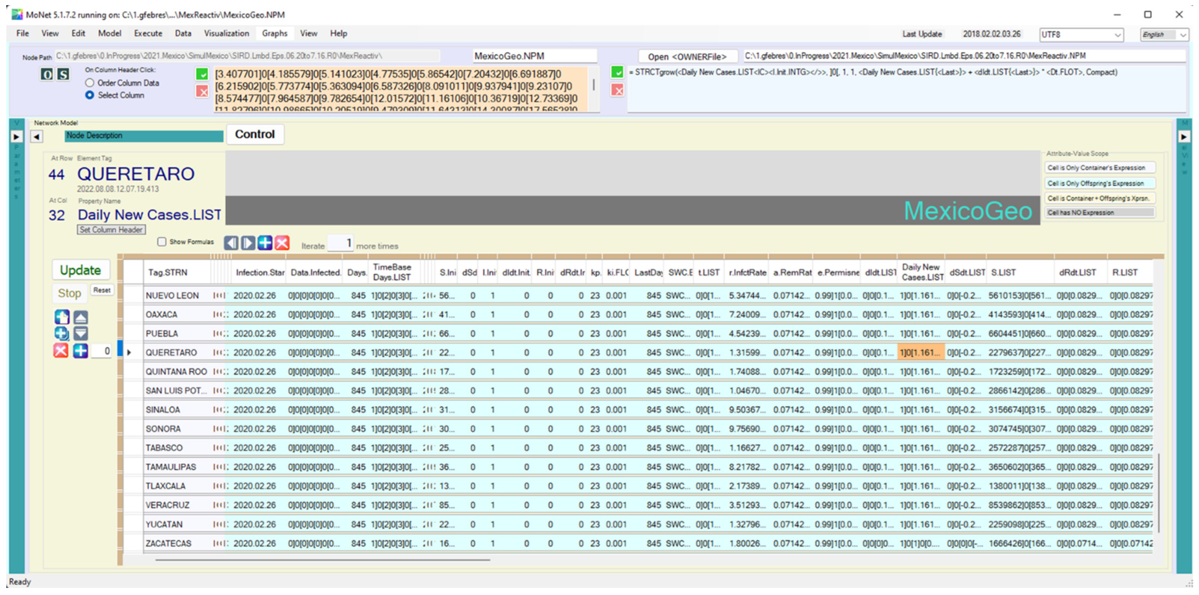
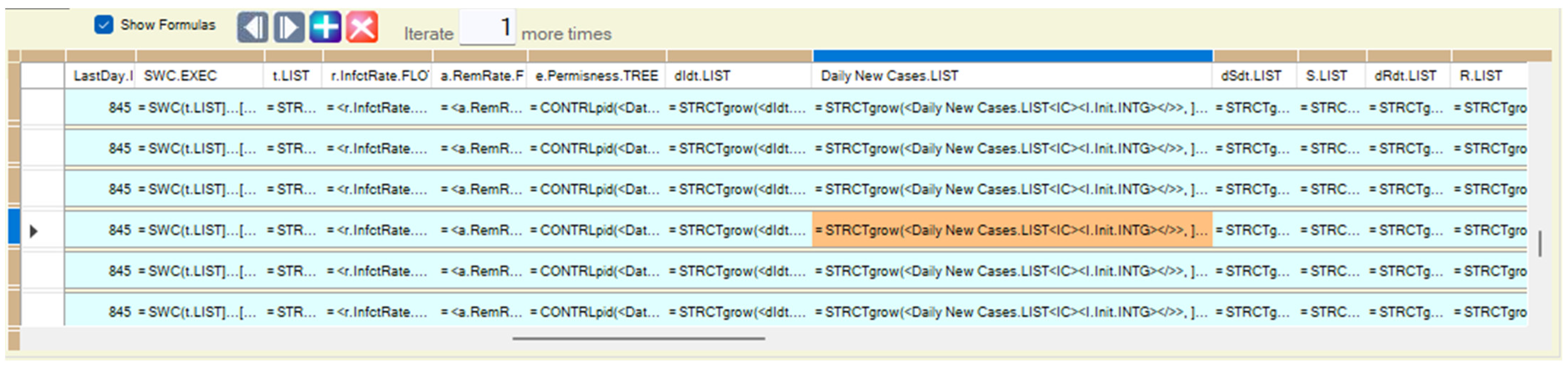
2.5. Monet, the Computing Environment, and DAR, the Data Autonomous Representation

Our implementation required handling several multidimensional numeric structures, each one representing an aspect of the modeled system. These structures need an identity as a whole, as there is the need to create mathematical operations where these structures are the operands. Lacking the possibility of directly handling complex structure operations would make this study difficult to manage. We used Monet as the simulation platform and its script language DAR (Data Autonomous Representation), which represents multidimensional numbers of any shape as a single identifiable compact parameter. The DAR language also allows for defining mathematical operations and algorithms where the arguments are complex structures.
To illustrate the simulation using Monet, take, for example, the solution by the simulation of the differential Equation (1a–d) that is all included in the ten cells of Monet’s interface grid shown in Figure 4. The cells under the column names Daily New Cases.LIST, S.LIST, and R.LIST contain the values of variables I , S , and R , while the cells under the column names dIdt.LIST, dSdt.LIST, and dRdt.LIST contain their corresponding derivatives with respect to time (t). Column e.Permisness.TREE contains the values regarding the PI-controlled variable v ( t ) . In columns r.InfctRate.FLOT and r.InfctRate.FLOT are the constant values of r and a .
The values in the cell may be a constant or may be the result of executing an expression associated with the cell. Explaining how the language DAR was used to write these expressions is beyond the scope of this document. However, to give an idea of how DAR works, we show the formula corresponding to the cell S.LIST, where the susceptible individuals are computed by integrating the values contained in cell dSdt.LIST:
<S.LIST> = STRCTgrow(<S.LIST<IC><S.Init.INTG></>>, ]0[, 1, 1, <S.LIST{<Last>}> + <dSdt.LIST{<Last>}> * <Dt.FLOT>, Compact)
The function STRCTgrow produces a growing list of elements, each with a value determined by the fourth argument; in this case: <S.LIST{<Last>}> + <dSdt.LIST{<Last>}> * <Dt.FLOT>. The elements are separated by the symbol ]0[ indicated in the second argument of the function. The first function’s argument points to the cell where the growing structure is located and the corresponding initial condition.
Encapsulating local computational problems and visually organizing parameters in the screen grid, in turn, reduces the complexity of the whole solution while making it possible to enlarge the model’s scope. The simulation of complex systems typically challenges the researcher with non-linear behavior, non-regular spaces, and the size of the system representation. When the target is to simulate many complex systems within the same computing environment, the challenge becomes larger up to another scale.
When the regions simulated can be described as the joint of smaller geographical regions, the functions included in Equation (1a–d) were computed by aggregating the simulation results obtained from the more detailed data of the internal geographical regions. Table A2, included in Appendix B, shows the calculation procedures involved in this alternative computation. The procedure Sum (summation) of the aggregated values is used when the value being processed is an absolute value. For intensive parameters, as the derivative terms, the procedure Avg (average) is used.

3. Results

3.1. Prognostics for 21 Days into the Future

This task was intended to prepare for the most likely growing infection rates and focus actions. The probability model expressed in Equation (8) was computed for Mexico and the geographical regions at a national scale and at a state scale showing results for each municipality. The resulting system was applied to the 32 Mexican states and their 2457 municipalities. Each probability model comprised more than 840 data points. The data were obtained from the web page COVID-19 México [23] prepared by the Mexican Consejo Nacional de Ciencia y Tecnología.
The projection time of 21 days was chosen. To make this choice, we first noticed the seven-day oscillation in the infection rates observed at all scales in Mexico. This weekly cycling behavior is present all around the world. The Appendix C includes graphs of the daily newly COVID-19-infected individuals for several countries, evidencing that this seven-day oscillatory pattern takes place in countries on all continents. Studies mentioning the seven-day oscillatory pattern consider that this behavior might be associated with epidemiological or social factors leading to a higher transmission on certain days (Bukhari et al. [25]) or that it might be associated with the weekday activity (Pavlicek et al. [26]) or with the reporting of the individual cases (Bergman et al. [27], for New York City and Los Angeles). However, a detailed look at the shapes of the oscillations reveals complex shapes which, in our opinion, suggest there are other dominant causes present in this phenomenon. Thus, we are not certain about the cause of these oscillations; that may be a matter of other research. However, we know that taking a time horizon multiple of seven days will favor the coherence of our results. Finally, we considered three weeks provide a reasonable time to react according to the projections produced. However, applying this procedure without additional modifications will produce oscillating prognostics that are inconvenient for interpreting the hardness of the possible upcoming conditions. Therefore, our results present the daily infected individuals averaged for the week centered 21 days into the future.
Figure 5 shows the daily infected individuals projection three weeks ahead of the current time for the states of Mexico (left) and the Federal District municipalities (right). The blue and red bubbles mean λ negative and positive values, thus signaling whether the number of daily infected individuals is decreasing or increasing. The areas of the bubbles are proportional to the population of the state or municipality represented.

3.2. Assessing the Precision of Prognostics

Since the projection model is an empirical probability model based on a status classifying and counting system, computing the error by considering theoretical error distributions does not apply. We see two types of deviations in the prognostics: (i) deviations of the math model compared to the reality, including Equation (1a–d) and the exponential growth model suggested for the number of newly infected individuals expressed in Equation (3); and (ii) differences between the discrete values assigned to the permissiveness v and growth parameter λ versus their actual values. Considering the diversity of the parameters affecting the precision of the simulation, we evaluated the goodness of the method by graphically comparing the 21-day projections. Figure 6 compares the data registered for the state of Queretaro with the 21-day projections obtained for the same data. On the left, Figure 6 shows the newly infected people that occurred. The figure in the Center shows the 21-day predictions performed from day 45 to 845 of the pandemic. The right graph shows the projection’s normalized error computed as (Projected Daily Infected − Daily Infected)/Daily Infected.
To compute the projections corresponding to the days in the past, the process depicted in Figure 3 was repeated for each past day. For every past day simulated, the probabilities computed rely on structure P, which must be fed with a past-time horizon of up to 800 days, depending on the data available. To avoid the need for memorizing a structure P, each day’s vector E is extracted from P and ‘multiplied’ by the growth factor vector G introduced in Equation (8). The result represents the probability that each scaled λ value will occur Δ t days into the future.
Comparing the left and center graphs in Figure 6, we observe two dimensions to assess the projection’s quality: the outer-scale process trend, and the inner-scale oscillation that we have referred to as the seven-day oscillation pattern. With the conditions of these simulations, the normalized error shown in the right graph in Figure 6 shows the outer-scale process trend established after day 180. Thereafter, the error rarely goes beyond the band of −0.2 to 0.2 while it progressively concentrates around the zero-error axis, confirming that an increase in the past-time horizon improves the quality of the pattern predictions.
The similarity between the original data (blue dots) and its counterpart prediction (purple dots) is remarkable. Figure 6 shows the specific case of Queretaro, but the similarity between the data and prediction graphs is evident in all the states and municipalities inspected.
An interesting aspect of the newly COVID-19-infected individuals is the shape of the infection curve that goes up and down in a seven-day period producing the sensation of more than one infection curve. There is only one curve, but a higher frequency oscillation makes it appear as more than one curve. Since the first stages of the pandemic, we noticed the seven-day oscillatory pattern in the number of newly infected individuals. The pattern is present in almost every continent, country, and region we have inspected. Up to the date of this study, we do not have an explanation for this. We have not had news about other explanations either. Nevertheless, for the present study, the relevant fact is that the model successfully captured the general tendency of the infected individuals and these oscillatory patterns.

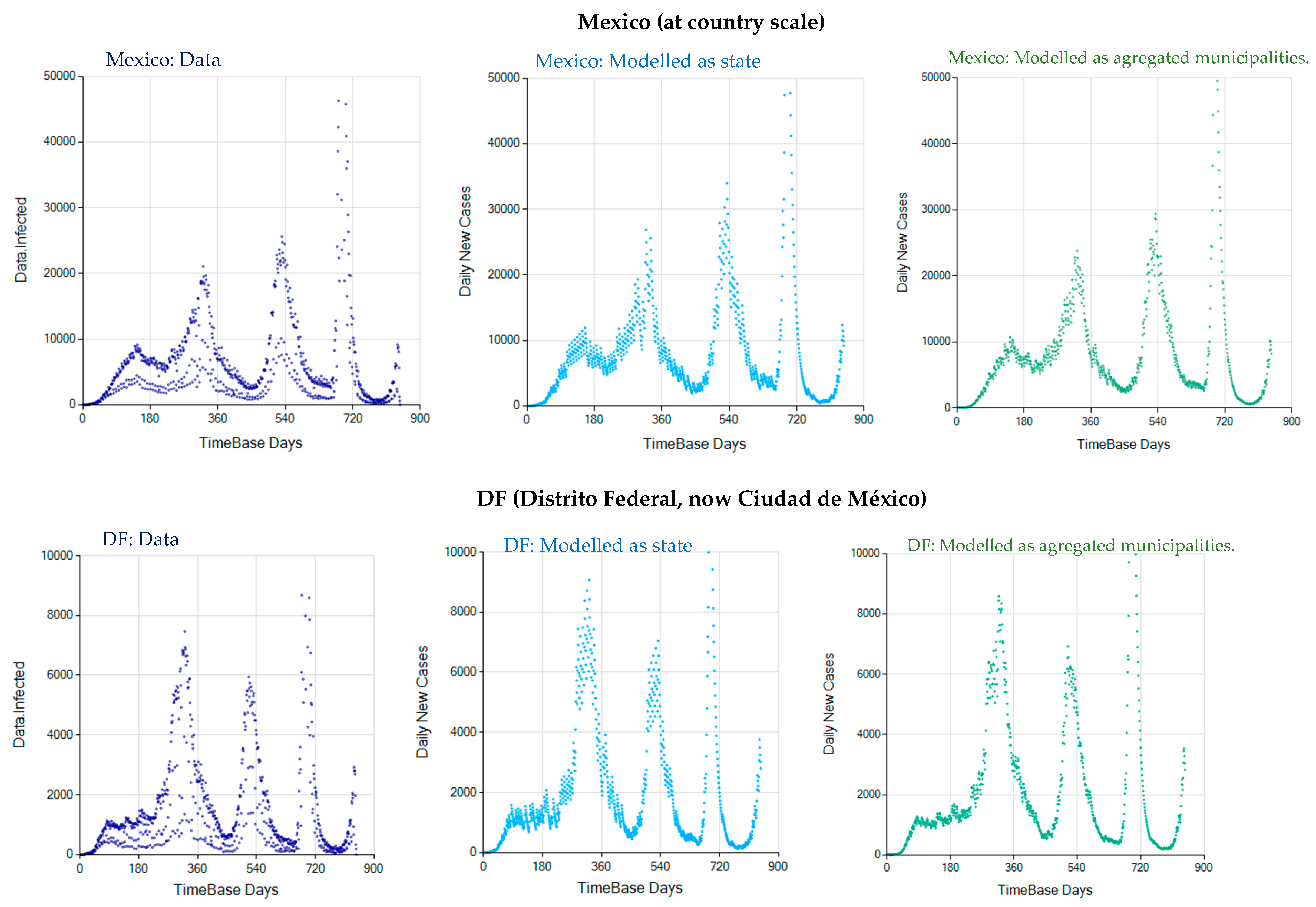
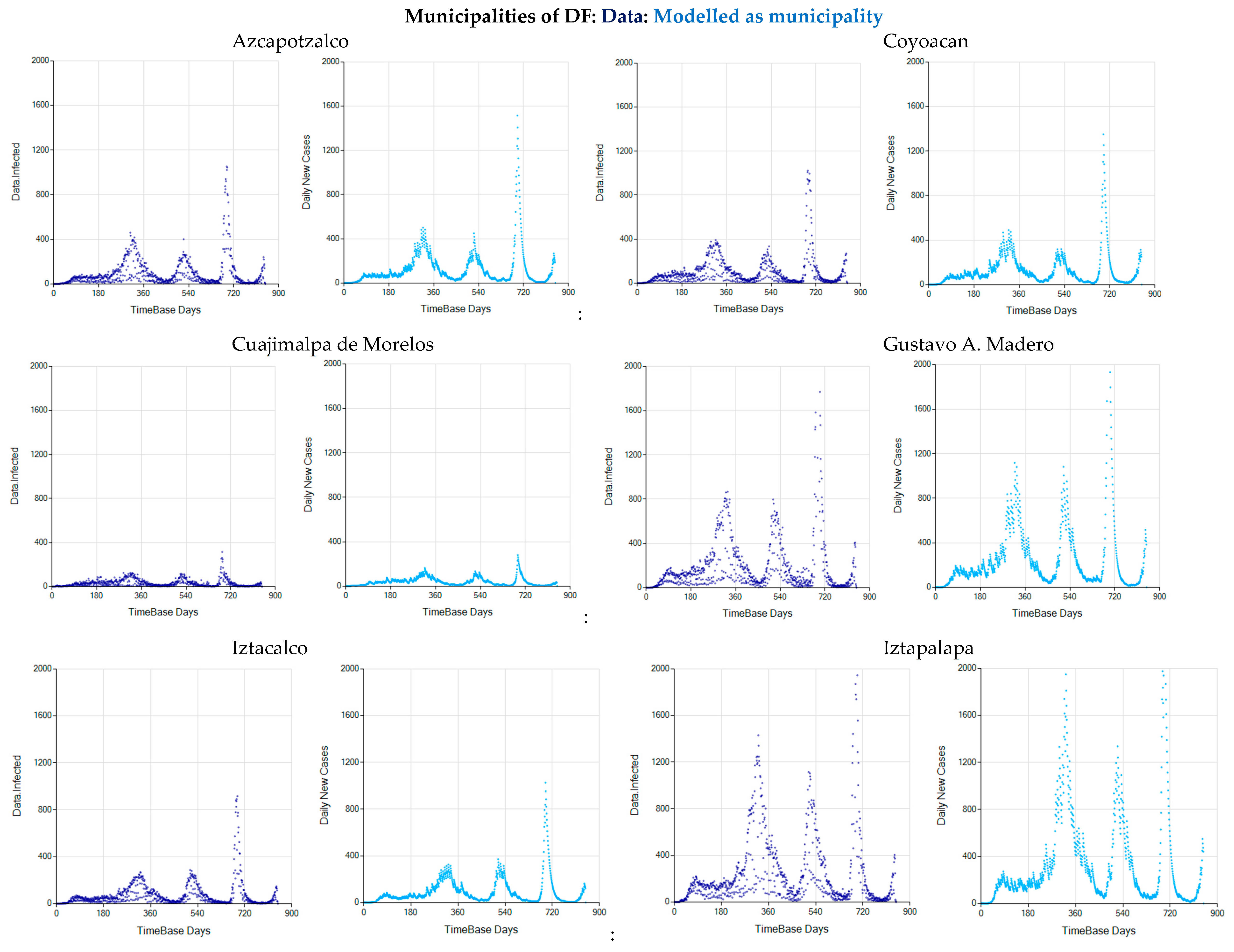
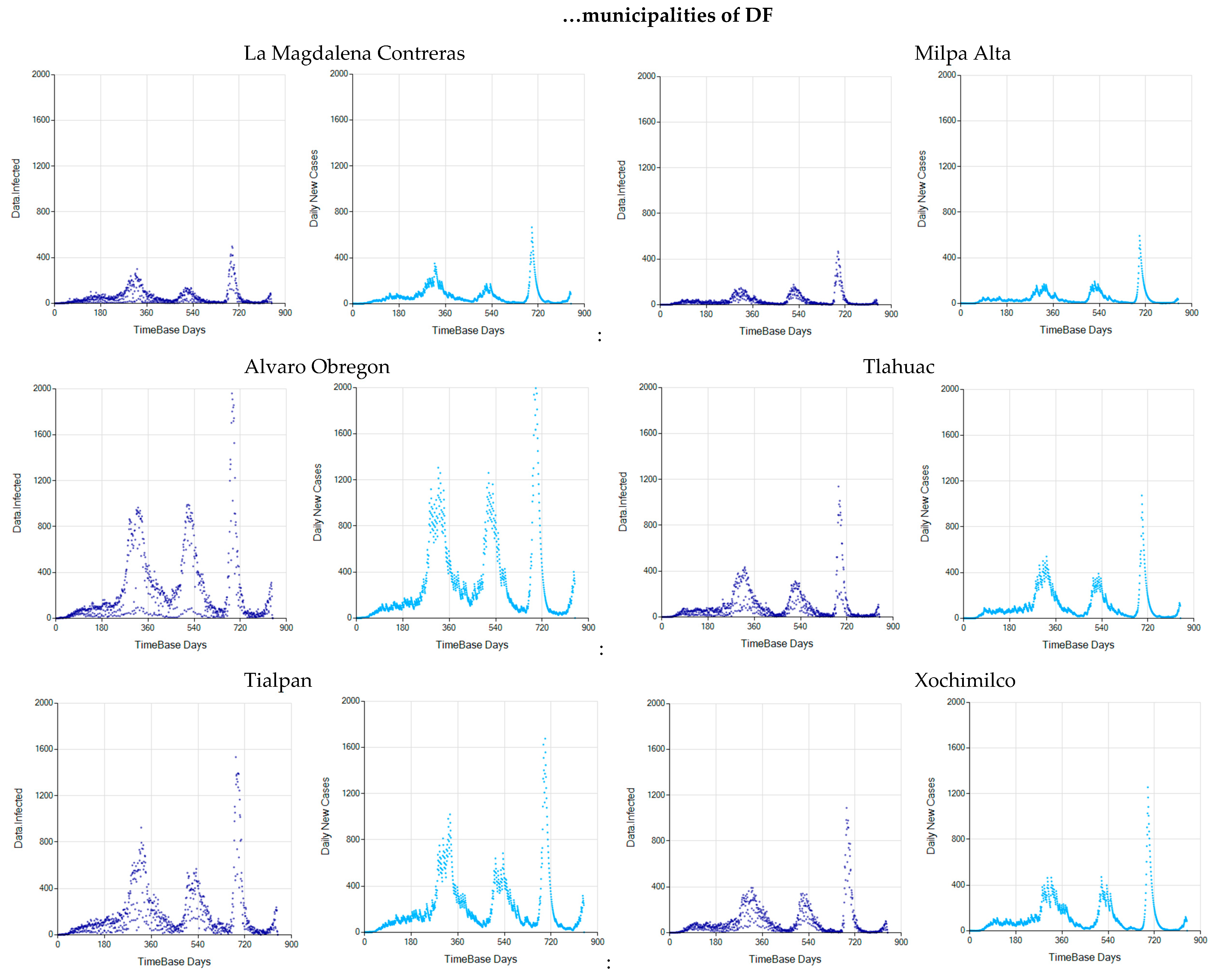
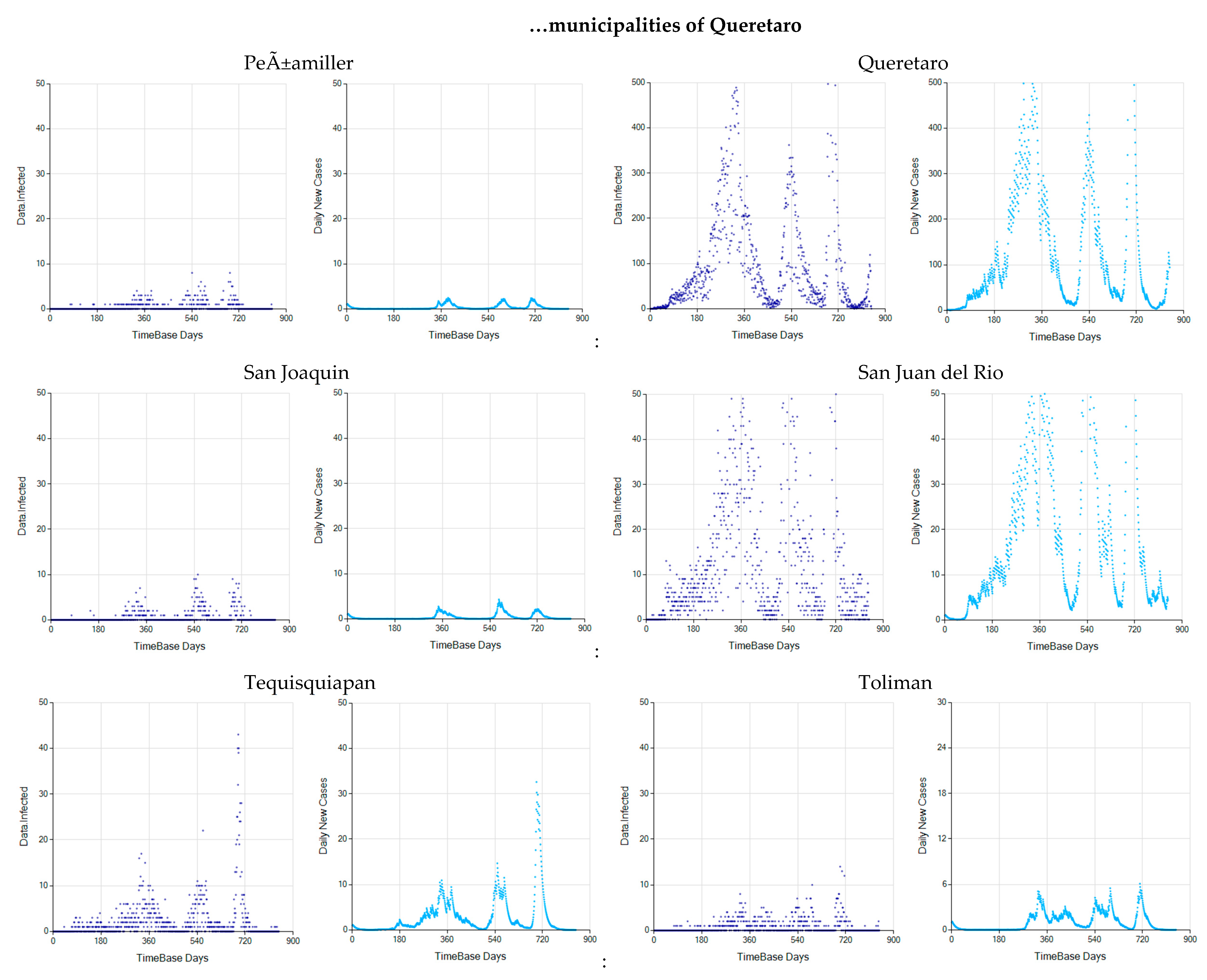
3.3. The Alternative of Aggregating More Detailed Region Values

Some graphs comparing the results obtained by (i) solving Equation (1a–d) using data at the scale of the geographical region being simulated, and by (ii) aggregating the results from the contained smaller geographical regions, are included in Appendix D. There is a notorious similarity between any two graphs corresponding to the same region. As could be expected, there is a loss of the oscillation patterns in the aggregated graphs due to the noise included in the aggregation process.

4. Generalizing the Method

We applied the projection model to the COVID-19 pandemic’s infection process. In most countries, but especially in Mexico, the evolution of the pandemic was registered with reliable, well-organized, and daily updated data [23]. These circumstances provided us with an excellent opportunity to develop and test this study’s projection method. This application of the method has its value. However, it is worth describing the method as a general procedure that is considered in situations comprising the required conditions. Figure 7 illustrates the general steps toward generalizing the method.

5. Discussion

A statistical–deterministic hybrid method was applied to simulate the COVID-19 infectious process and to forecast the number of daily new infected individuals. Taking advantage of the rigorous available data for every state and municipality of Mexico, and relying on the capabilities of Monet [22], we simulated 2490 instances of the model to rank the 32 states, the 2447 municipalities, and the country, in the sense of the expected infection growth. Some conditions are required to apply the method.
Apart from the fact of not including the asymptomatic individuals, which we have little control of, the application of the method to predict the forthcoming infected individuals after the prediction time Δ t would need one to assume future values for the permissiveness function v ( t ) . This may look like a limitation. However, the permissiveness function is the reflex, at least partially, of the government’s decisions and actions. Thus, the method offers the possibility to assess the likely impact of modifying social activity to control the COVID-19 infection process.
As in any probability-based predictor method, some volume of registered data is required to produce reliable results. With the conditions of the simulations, the outer-scale process predictions required about 180 data points. The reproduction of the inner-scale oscillation pattern also requires 180 data points, but the reproduction of the pattern seems to improve indefinitely as the number of points increases. Using the outer-scale process as reference, we conjecture that the data points needed are about nine times the time into the future to prognosticate. By intuition, we know the proportion varies with the number of dimensions of the probabilistic model. This study’s model is two dimensional. Thus, we propose the following rule to estimate the number of data points dp needed to reach good quality predictions as a function of prediction time Δ t and the number of dimensions dim of the probabilistic model:
d p 3 d i m · Δ t     .
The requirements of the data, growing exponentially with the number of past dimensions (dim) related to the prognostic, is obviously a limitation of the method. Nevertheless, the hybridization of the statistical data with the SIR model makes the data requirements approximated in Equation (10) lower than the data requirements that most time-series projection methods would otherwise require. A drawback of the method related to the data considered manifests when the status ( λ i ,   v j ) at any time t appears for the first time in the registered data. Then, the probabilities at the status are not observable, and thus the prediction based on a previously experienced status is impossible. Since the number of statuses represented in the model is m n (the product of the resolutions of λ and v ), registering data large enough to cover all statuses at least once is not feasible. This is why some points in the center graph of Figure 6 lay on the horizontal axis, meaning there is no prediction corresponding at these times.
Besides the sufficient data points, every new application requires a fine-tuning process to make the most of the simulator. Especially, the model’s PI controller must be tuned to obtain good results. Additionally, applying the method to study many instances of the same model, as in the present study, requires tools to handle multidimensional structures representation, operations, and registering. Once these requirements are fulfilled, the method can be massively applied in an integrated simulator.
The projection results proved to follow the general tendency of the process, with its waves and valleys, and at the same time reproduce the inner scale system’s dynamics represented by the observed weekly oscillations. We regard this as an interesting result since the projection models we know about either capture the general tendency or the inner dynamics as a process fingerprint, but not both at the same time. The capability of simultaneously forecasting a set of different scenarios leads to the possibility of creating prediction landscapes. Finally, we regard the capacity to capture the system’s large-scale trends as well as its more detailed local characteristic dynamics as a relevant result, since it places this method as an effective tool to study non-linear systems.
More than two years after the pandemic declaration, the daily COVID-19 death toll seems to be slowly reducing. The vaccination campaigns, the improvement of the disease treatment, and better logistical operations in hospitals are some of the reasons for this achievement. Additionally, as Rypdal [14] suggests, the increase in the number of cases related to more resilient lower-aged individuals contributes to lowering the death ratio. Additionally, unfortunately, many of the most vulnerable people already died, so the reduction might be also partly explained by survival bias. The infection process, however, does not show similar progress. Infection waves continue to emerge in all states and municipalities of Mexico. At the end of each wave, where we could talk about valleys, the number of infected individuals is closer to zero, repeatedly tempting us to think the epidemics will shortly finish. However, as Figure 6 illustrates for a specific state (one could see the similar behavior in any other state), a new infection wave is beginning in Queretaro, and there is no indication of these waves dissipating in the near future.

Author Contributions

Conceptualization, G.L.F. and C.G.; methods, G.L.F.; software, G.L.F.; writing, G.L.F. and C.G. All authors have read and agreed to the published version of the manuscript.

Funding

This research received no external funding.

Conflicts of Interest

The authors declares no conflict of interest.

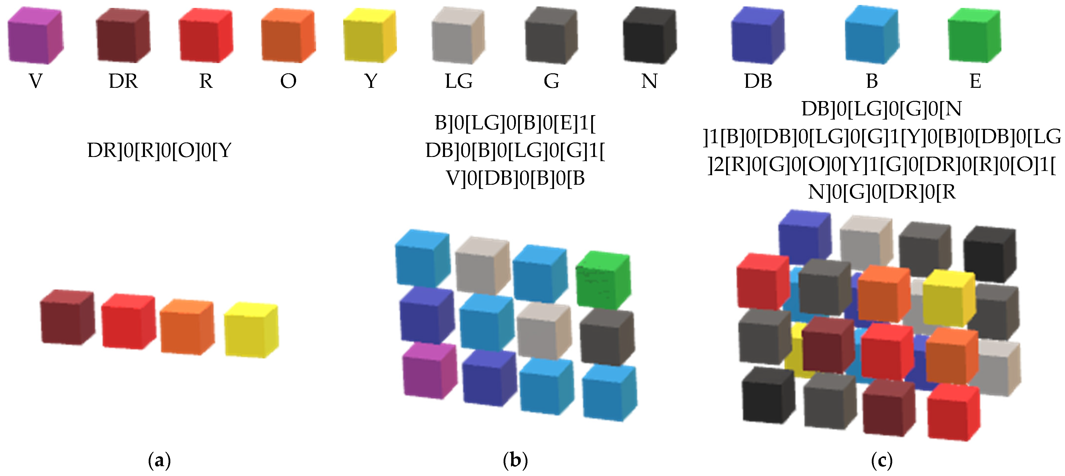
Appendix A. The Data Autonomous Representation

The Data Autonomous Representation (DAR) is a script language specially designed to handle information elements in a multidimensional logical environment. DAR consists of a set of rules and syntaxes that allow for depicting and registering complex data structures. DAR includes the possibility for constructing arithmetic operations and functions defined over the space of multidimensional arguments. DAR handles three types of complex structure topologies: ORTHOs, TREEs, and RINGs. These three types of structures are regarded as the prime types of structures that, when properly combined, can describe any complex data structure.
As a rule that applies to all structures, DAR uses special symbols to split elementary components that form a compound multidimensional structure. The splitting symbols are of the form ‘]d[‘. The opening and closing brackets (in that order) suggest the sides where the elements are being separated. The letter ‘d’ is the number of the dimensions that the splitting symbol ‘]d[‘refers to. The splitting dimension tag ‘d’ starts with the number zero (0).
Figure A1. The color-property description of ORTH-structures of objects of one, two and three dimensions. The particular case of one-dimension-ORTH can also be considered a LIST.
Systems 10 00138 g0a1
Figure A1 shows examples of ORTH structures in one, two and three dimensions (a figurative version).
Since ORTHOs are perhaps the most frequently used data structure, this appendix expands the explanation about them. ORTHOs: To this type belongs any structure being formed by the same number of elements counted within any of the structure dimensions. Thus, ORTHOs are regular sets of elements showing structural symmetry around any plane oriented perpendicular to the direction of each dimension. To describe
One-dimensional structure, in Figure A1a:
DR]0[R]0[O]0[Y
Two-dimensional structure, in Figure A1b:
B]0[LG]0[B]0[E]1[DB]0[B]0[LG]0[G]1[V]0[DB]0[B]0[B
Three-dimensional structure, in Figure A1c:
DB]0[LG]0[G]0[N]1[B]0[DB]0[LG]0[G]1[Y]0[B]0[DB]0[LG]2[R]0[G]0[O]0[Y]1[G]0[DR]0[R]0[O]1[N]0[G]0[DR]0[R
Extracting sub-structures: A very useful tool that DAR offers is the extracting sub-structures feature. Extracting sub-ORTH structures is done using the Range-Limit-Splitting symbol ‘]…[‘. The Range-Limit-Splitting symbol indicates that all the elements located within the range limits indicated at the start and the end of the splitting symbol are included in the selection. Thus, the extractor phrase {L]…[U} means that all the elements located above (or equal to) the lower limit L, and below (or equal to) the upper limit U are included in the structure extraction. The coordinate’s limits L and U refer to the corresponding dimension of the subject structure. The limits of the multidimensional ORTH structures are also specified using the two-dot dimension-splitting symbol (:). The general extracting phrase {L0:L1:L2]…[U0:U1:U2} means that the elements within the limits specified for dimensions zero, one, and two, respectively, are to be selected. An example helps to understand the syntax. Extracting the eight elements of the close-plane lower two rows of Figure A1c implies the following syntax:
G]0[DR]0[R]0[O]1[N]0[G]0[DR]0[R = <Figure.A1c{0:0:0]…[3:1:0}>
The extracted structure is shown in Figure A2.
Figure A2. A substructure extracted from the structure shown in Figure A1c.
Systems 10 00138 g0a2
This syntax for specifying sub-ORTHs of any ORTH is applicable to ORTHs of any number of dimensions. The number of splitting dimension symbols ‘:’ in the extracting phrase indicates the number of dimensions (minus one) of the subject structure, therefore meaning these two numbers must match.

Appendix B. Integrating Differential Equations with Monet

Appendix B.1. Computing Models Using Data at the Corresponding Scale

Monet is an effective tool to solve differential equations by articulating and integrating differential expressions. Monet’s environment organizes expressions in arrays of cells. The cells can allocate multidimensional expressions including orthogonal and tree-like structures. Therefore, a complete list of values representing a time series of the daily newly infected individuals is stored in a single cell. Six cells are required to model the core of Equation (1a–d). As illustrated in Figure A3 and Figure A4, these cells store the values for the time series corresponding to d S d t , S , d I d t , I , d R d t , and R . In the simulation, the variable I is named ‘Daily New Cases.LIST’. Table A1 shows the procedures applied to compute the variables of the Equation (1a–d):
Table A1. Main procedures involved in integrating differential Equation (1a–d).
<dIdt.LIST>= STRCTgrow(<dIdt.LIST<IC><dIdt.Init.FLOT></>>, ]0[, 1, 1, <r.InfctRate.FLOT{<Last>{0<RelDepth>0</>}}> * <e.Permness.TREE{<Last>{0<RelDepth>0</>}}> * <S.LIST{<Last>}> * <Daily New Cases.LIST{<Last>}> - <a.RemRate.FLOT> * <Daily New Cases.LIST{<Last>}>, Compact)
<Daily New Cases.LIST>= STRCTgrow(<Daily New Cases.LIST<IC><I.Init.INTG></>>, ]0[, 1, 1, <Daily New Cases.LIST{<Last>}> + <dIdt.LIST{<Last>}> * <Dt.FLOT>, Compact)
<dSdt.LIST>= STRCTgrow(<dSdt.LIST<IC><dSdt.Init.FLOT></>>, ]0[, 1, 1, -1 * <e.Permissiveness.TREE{<Last>{0<RelDepth>0</>}}> * <r.InfctRate.FLOT{<Last>{0<RelDepth>0</>}}> * <S.LIST{<Last>}> * <Daily New Cases.LIST{<Last>}>, Compact)
<S.INTG>= STRCTgrow(<S.LIST<IC><S.Init.INTG></>>, ]0[, 1, 1, <S.LIST{<Last>}> +<dSdt.LIST{<Last>}> * <Dt.FLOT>, Compact)
<dRdt.LIST>= STRCTgrow(<dRdt.LIST<IC><dRdt.Init.FLOT></>>, ]0[, 1, 1, <a.RemRate.FLOT> * <Daily New Cases.LIST{<Last>}>, Compact)
<R.LIST>= STRCTgrow(<R.LIST<IC><R.Init.INTG></>>, ]0[, 1, 1, <R.LIST{<Last>}> +<dRdt.LIST{<Last>}> * <Dt.FLOT>, Compact)
The procedure STRCTgrow() used to determine the components of the Equation (1a–d) builds a time series with the values of each equation’s component. To do so, every time the simulation goes over the procedure STRCTgrow(), a new element is added to the LIST structure representing the time series. The value of the element just added is computed as the procedure’s argument indicates. When necessary, an expression of the form <IC>InitialConditionValue</> guides the procedure towards the initial conditions of each parameter. Performing these operations successively, the differential terms are computed and integrated into the final solution of the differential equation. The elements forming the resulting functions are separated by the split symbol ‘]0[‘.
Monet stores procedures into cells to control the procedures stored in other cells. The procedure SWC (Step Wise Compute) serves to coordinate the calculation of the rows stored to model COVID-19 for each Mexican region. In the Column tagged as SWC.EXEC is stored in the procedure text to execute the computation of the values included in the argument expression t.LIST]…[R.LIST. The split expression ]…[ returns all the values in the range from t.LIST to R.LIST.
<SWC.EXEC> = SWC(t.LIST]…[R.LIST, 1, <Days.INTG> − <LastDay.INTG>, <Reset> = False, LastDay.INTG).
The other parameters indicate the size of discrete differential time, the number of times the cycling calculation is performed, and a switch to continue the calculus from the time registered in LastDay.INTG or from the very simulation beginning applying initial conditions, and finally the name of the column (LastDay.INTG) where the last processing time is stored.
Figure A3. A view of Monet’s interface.
Systems 10 00138 g0a3
Figure A4. A detail of Monet’s interface grid with the Show Formulas option activated.
Systems 10 00138 g0a4

Appendix B.2. Computing Models Aggregating Results from Inner Detailed Scale

An alternative calculation process was performed by aggregating the simulation results obtained with the more detailed data referring to the next inner geographical region. Table A2 shows the procedures involved in this alternative computation. The Sum of the aggregated values is used when the value being processed is an absolute value. When the value being processed is an intensive parameter, as the derivative terms, the procedure Avg (average) is used.
Table A2. Main procedures involved in integrating Differential Equation (1a–d).
<dIdt.LIST>= Avg(<dIdt.LIST><~><OFFSPRINGS>.<LEAF></~>, <void>)
<Daily New Cases.LIST>= Sum(<Daily New Cases.LIST><~><OFFSPRINGS>.<LEAF></~>, <void>)
<dSdt.LIST> = Avg(<dIdt.LIST><~><OFFSPRINGS>.<LEAF></~>, <void>)
<S.INTG>= Sum(<Daily New Cases.LIST><~><OFFSPRINGS>.<LEAF></~>, <void>)
<dRdt.LIST>= Avg(<dIdt.LIST><~><OFFSPRINGS>.<LEAF></~>, <void>)
<R.LIST>= Sum(<Daily New Cases.LIST><~><OFFSPRINGS>.<LEAF></~>, <void>)

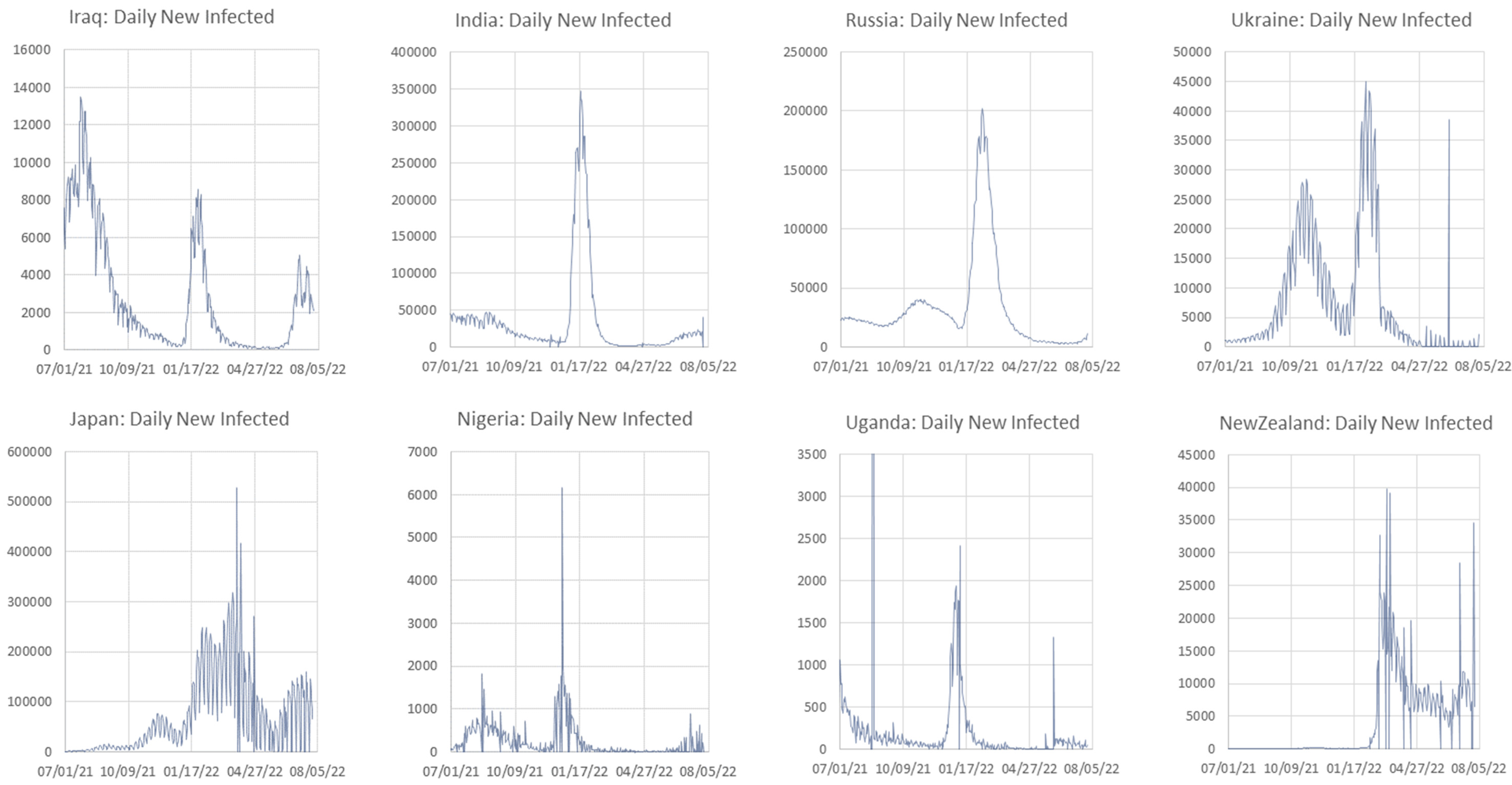
Appendix C. Graphs of Daily New Infected Individuals

Figure A5. Graphs of COVID-19 Daily New Infected individuals for several countries. The purpose is to establish evidence that the seven-day oscillatory pattern takes place in countries on all continents.
Systems 10 00138 g0a5aSystems 10 00138 g0a5b

Appendix D. Daily New Infected Model Computed at Different Scales

Figure A6. Graphs of Daily New Infected individuals are included for Mexican regions at the scale of Country, States and Municipalities. Graphs show the result of models computed with data at different scales and as the aggregated values of the models at the more detailed scale.
Systems 10 00138 g0a6aSystems 10 00138 g0a6bSystems 10 00138 g0a6cSystems 10 00138 g0a6dSystems 10 00138 g0a6eSystems 10 00138 g0a6fSystems 10 00138 g0a6g

References

  1. Kermack, W.; McKendrick, A. Contributions to the mathematical theory of epidemics—I. Bull. Math. Biol. 1991, 53, 33–55. [Google Scholar] [CrossRef]
  2. Planas, D.; Veyer, D.; Baidaliuk, A.; Staropoli, I.; Guivel-Benhassine, F.; Rajah, M.M.; Planchais, C.; Porrot, F.; Robillard, N.; Puech, J.; et al. Reduced sensitivity of SARS-CoV-2 variant Delta to antibody neutralization. Nature 2021, 596, 276–280. [Google Scholar] [CrossRef] [PubMed]
  3. Sofonea, M.T.; Roquebert, B.; Foulongne, V.; Morquin, D.; Verdurme, L.; Trombert-Paolantoni, S.; Roussel, M.; Bonetti, J.-C.; Zerah, J.; Haim-Boukobza, S.; et al. Analyzing and Modeling the Spread of SARS-CoV-2 Omicron Lineages BA.1 and BA.2, France, September 2021–February 2022. Emerg. Infect. Dis. 2022, 28, 1355–1365. [Google Scholar] [CrossRef] [PubMed]
  4. Fourati, S.; Gautier, G.; Chovelon, M.; Soulier, A.; N’Debi, M.; Demontant, V.; Kennel, C.; Rodriguez, C.; Pawlotsky, J.-M. Persistent SARS-CoV-2 Alpha Variant Infection in Immunosuppressed Patient, France, February 2022. Emerg. Infect. Dis. 2022, 28, 1512–1515. [Google Scholar] [CrossRef]
  5. Pulliam, J.R.C.; van Schalkwyk, C.; Govender, N.; von Gottberg, A.; Cohen, C.; Groome, M.J.; Dushoff, J.; Mlisana, K.; Moultrie, H. Increased risk of SARS-CoV-2 reinfection associated with emergence of Omicron in South Africa. Science 2022, 376, eabn4947. [Google Scholar] [CrossRef]
  6. Silverman, R.A.; Ceci, A.; Cohen, A.; Helmick, M.; Short, E.; Bordwine, P.; Friedlander, M.J.; Finkielstein, C.V. Vaccine Effectiveness during Outbreak of COVID-19 Alpha (B.1.1.7) Variant in Men’s Correctional Facility, United States. Emerg. Infect. Dis. 2022, 28, 1313–1320. [Google Scholar] [CrossRef]
  7. Matsumura, Y.; Nagao, M.; Yamamoto, M.; Tsuchido, Y.; Noguchi, T.; Shinohara, K.; Yukawa, S.; Inoue, H.; Ikeda, T. Transmissibility of SARS-CoV-2 B.1.1.214 and Alpha Variants during 4 COVID-19 Waves, Kyoto, Japan, January 2020–June 2021. Emerg. Infect. Dis. 2022, 28, 1569. [Google Scholar] [CrossRef]
  8. Khateeb, D.; Gabrieli, T.; Sofer, B.; Hattar, A.; Cordela, S.; Chaouat, A.; Spivak, I.; Lejbkowicz, I.; Almog, R.; Mandelboim, M.; et al. SARS-CoV-2 variants with reduced infectivity and varied sensitivity to the BNT162b2 vaccine are developed during the course of infection. PLOS Pathog. 2022, 18, e1010242. [Google Scholar] [CrossRef]
  9. Menendez, J. Elementary Time Delay Dynamics of COVID-19 disease. medRxiv 2020. [Google Scholar] [CrossRef]
  10. Ebraheem, H.K.; Alkhateeb, N.; Badran, H.; Sultan, E. Delayed Dynamics of SIR Model for COVID-19. Open J. Model. Simul. 2021, 09, 146–158. [Google Scholar] [CrossRef]
  11. Hale, T.; Angrist, N.; Hale, A.J.; Kira, B.; Majumdar, S.; Petherick, A.; Phillips, T.; Sridhar, D.; Thompson, R.N.; Webster, S.; et al. Government responses and COVID-19 deaths: Global evidence across multiple pandemic waves. PLoS ONE 2021, 16, e0253116. [Google Scholar] [CrossRef] [PubMed]
  12. University of Oxford. OXFORD COVID-19 Government Response Stringency Index. Available online: https://data.humdata.org/dataset/oxford-covid-19-government-response-tracker (accessed on 30 May 2022).
  13. Rypdal, K.; Bianchi, F.M.; Rypdal, M. Intervention Fatigue is the Primary Cause of Strong Secondary Waves in the COVID-19 Pandemic. Int. J. Environ. Res. Public Health 2020, 17, 9592. [Google Scholar] [CrossRef] [PubMed]
  14. Rypdal, K. The Tipping Effect of Delayed Interventions on the Evolution of COVID-19 Incidence. Int. J. Environ. Res. Public Health 2021, 18, 4484. [Google Scholar] [CrossRef]
  15. Febres, G.L. Assessing the Impact of Social Activity Permissiveness on the COVID-19 Infection Curve of Several Countries. arXiv 2021, arXiv:2106.04085v2. [Google Scholar]
  16. Kiselev Ilya, R.; Kolpakov, F.I.A. A Delay Differential Equation approach to model the COVID-19 pandemic. medRxiv 2021. [Google Scholar] [CrossRef]
  17. HDX. Center for Humanitarian Data. Available online: https://data.humdata.org/dataset/novel-coronavirus-2019-ncov-cases (accessed on 1 July 2022).
  18. Lux, T.M.; Marchesi, M. Scaling and criticality in a stochastic multi-agent model of a financial market. Nature 1999, 397, 498–500. [Google Scholar] [CrossRef]
  19. Borland, L. Exploring the dynamics of financial markets: From stock prices to strategy returns. Chaos Solitons Fractals 2016, 88, 59–74. [Google Scholar] [CrossRef]
  20. Total COVID-19 Tests. Comparisons across Countries are Affected by Differences in Testing Policies and Reporting Methods. Available online: https://ourworldindata.org/grapher/full-list-total-tests-for-covid-19 (accessed on 30 May 2022).
  21. COVID-19 Dashboard by the Center for Systems Science and Engineering (CSSE) at Johns Hopkins University (JHU). Available online: https://coronavirus.jhu.edu/map.html (accessed on 30 May 2022).
  22. Febres, G.L. Dynamic Adjustment of SIR Model with the Social Permissiveness: An Actual Measure of the Infection Rate. arXiv 2021, arXiv:2106.04085. [Google Scholar]
  23. COVID-19 México. Available online: https://datos.covid-19.conacyt.mx/#DOView (accessed on 30 May 2022).
  24. Febres, G.L. Basis to Develop a Platform for Multiple-Scale Complex Systems Modeling and Visualization: MoNet. arXiv 2017, arXiv:1701.04064. [Google Scholar]
  25. Bukhari, Q.; Jameel, Y.; Massaro, J.M.; D’Agostino, R.B.; Khan, S. Periodic Oscillations in Daily Reported Infections and Deaths for Coronavirus Disease 2019. JAMA Netw. Open 2020, 3, e2017521. [Google Scholar] [CrossRef]
  26. Pavlíček, T.; Rehak, P.; Král, P. Oscillatory Dynamics in Infectivity and Death Rates of COVID-19. mSystems 2020, 5, e00700-20. [Google Scholar] [CrossRef] [PubMed]
  27. Bergman, A.; Sella, Y.; Agre, P.; Casadevall, A. Oscillations in U.S. COVID-19 Incidence and Mortality Data Reflect Diagnostic and Reporting Factors. mSystems 2020, 5, e00544-20. [Google Scholar] [CrossRef] [PubMed]
Figure 1. COVD-19 correlation diagrams for daily new cases in Mexico, USA, Germany, Japan, Nigeria, and Iraq. Correlations computed with data from 1 April 2020 to 31 May 2021.
Systems 10 00138 g001
Figure 2. Daily new infected for the state Puebla, Mexico. The top-left graph shows the new daily infected for 845 days registered starting from the 26 February 2020. The graph in the middle presents the daily infected individuals obtained from the simulation of Equation (1a–d). The right graph presents the permissiveness. The bottom row presents the same parameters in a detailed time scale.
Systems 10 00138 g002
Figure 3. Schema of the use of past-time horizon data and projection time for the population of structure P.
Systems 10 00138 g003
Figure 4. Monet’s user interface detail showing cells devoted to the solution of Equation (1a–d) for a single Mexican state.
Systems 10 00138 g004
Figure 5. Projections of daily infected individuals and infection growth parameter. (Left) projections for the states of Mexico. (Right) projections for the municipalities of DF (Distrito Federal, now Ciudad de México). The vertical axis shows the average daily infected individuals expected for the week centered 21 days after the most recent data registered day (20 June 2022). The horizontal axis represents the current λ value.
Systems 10 00138 g005
Figure 6. A retrospective view of the 21-day projections compared with the number of newly infected individuals registered during the past year. The graphs correspond to the state of Queretaro during the 800 days prior to 20 June 2022, which is the last day in both graphs. On the left graph, the blue dots represent the number of newly infected individuals registered when each day arrived on time. On the center graph, the purple dots are the newly infected individuals projected 21 days ahead of each date. The right graph shows the projection’s normalized error.
Systems 10 00138 g006
Figure 7. Steps of the generalized projection method.
Systems 10 00138 g007
Publisher’s Note: MDPI stays neutral with regard to jurisdictional claims in published maps and institutional affiliations.

