A Robust Possibilistic Programming Approach for a Road-Rail Intermodal Routing Problem with Multiple Time Windows and Truck Operations Optimization under Carbon Cap-and-Trade Policy and Uncertainty

Abstract

This study investigates a road-rail intermodal routing problem in a hub-and-spoke network. Carbon cap-and-trade policy is accommodated with the routing to reduce carbon dioxide emissions. Multiple time windows are employed to enhance customer flexibility and achieve on-time pickup and delivery services. Road service flexibility and resulting truck operations optimization are explored by combining truck departure time planning under traffic restrictions and speed optimization with the routing. To enhance the feasibility and optimality of the problem optimization, the routing problem is formulated in a fuzzy environment where capacity and carbon trading price rate are trapezoidal fuzzy parameters. Based on the customer-centric objective setting, a fuzzy nonlinear optimization model and its linear reformation are given to formulate the proposed routing problem that combines distribution route design, time window selection and truck operations optimization. A robust possibilistic programming approach is developed to optimize the routing problem by obtaining its robust solutions. A case study is presented to demonstrate the feasibility of the proposed approaches. The results show that the multiple time windows and truck operations optimization can lower the total costs, enhance the optimality robustness and reduce carbon dioxide emissions of the routing optimization. The sensitivity analysis finds that increasing the lower bound of the confidence level in the robust possibilistic programming model improve the robustness and environmental sustainability; however, worsen the economy of the routing optimization.

1. Introduction

By using a hub-and-spoke network, road-rail intermodal transportation combines road pickup and delivery services with long-distance transportation by rail to provide customers with door-to-door transportation services. It takes advantage of the good flexibility, mobility and accessibility of road, and meanwhile benefits from the high-cost efficiency and environmental sustainability of rail that yields economics of scale [1]. Therefore, it is an effective option to take the place of low-efficient unimodal road transportation that still dominates the freight industry in Europe [2] and China [3], and provides a promising solution to establish an efficient and sustainable logistics system that supports globalization and international trade [4]. In such a transportation system, drayage operators transport goods between intermodal terminals, origins and destinations by road, terminal operators transship goods between road and rail, network operators use rail transportation to transport goods between intermodal terminals, and intermodal operators represent customers and collaborate with the above players to provide customers with transportation services [5]. Therefore, efficient operations of the transportation system need collaboration among various actors and stakeholders [6].

Transportation planning lays a powerful support for improving the operations of transportation systems. Intermodal operators can effectively realize the above-mentioned collaboration to provide customers with the best transportation services by the operational-level container routing. Routing optimization has been widely acknowledged to play a critical role in optimizing the operations of the intermodal transportation system [7], and has been highlighted by the transportation network planning as a research hotspot [8]. Notably, in long-distance and bulk transportation, road-rail intermodal transportation is costly and time consuming [9]. It also produces large amounts of greenhouse gases and is faced with considerable risks in the dynamic and uncertain environment [4]. Road-rail intermodal routing can provide a solid solution for intermodal operators to respond to above challenges. Therefore, this study explores this problem with the aim of improving the comprehensive performance of the transportation systems and provide customers with the best transportation services. Moreover, the proposed routing problem is from the perspective of the intermodal operator that represents customers and collaborates with various players in transportation.

The goal of the proposed routing is to help the intermodal operator to make the optimal routing decision to accomplish the transportation orders and satisfy the customer demands. To provide customers with the best transportation services, customer-centric objectives should be the foundation of the proposed routing. Logistical costs are the primary influencing factor that decides customers’ choice of transportation services provided by intermodal operators [10]. Therefore, the minimum-cost intermodal routing problems have been paid great attention by both early-stage studies [11,12] and recent literature [13,14]. Nowadays, transportation is widely integrated with agile manufacturing, speed-to-market deliveries and efficient supply chain management [15]. When choosing intermodal transportation services, an increasing number of customers are concerned with the quality of service that covers not only costs but also timeliness, risks and other indicators.

Furthermore, the transportation sector is a major contributor to carbon dioxide emissions that cause global warming and harm the sustainable development of human beings. Therefore, European Commission promises to reduce the carbon dioxide emissions in transportation by 60% by 2025, and China implemented the “Carbon Peak and Carbon Neutrality” policy in which freight transportation is treated as an important source of achieving the policy goals [16]. Road-rail intermodal transportation should consider the public goal of reducing carbon dioxide emissions in its routing to further empower the advantage it has of being more eco-friendly. Although customers pay less attention to the environmental impacts when choosing transportation services [10], carbon reduction policies (e.g., tax policy and cap-and-trade policy) implemented by large numbers of countries convert emissions into logistical costs, which draws attention from customers who are sensitive to the costs of the transportation services. Consequently, reducing carbon dioxide emissions is also included in the customer-centric objective setting of the proposed routing. Although less considered by the intermodal transportation planning compared with the carbon tax policy, the carbon cap-and-trade policy in recent years is acknowledged to be more efficient in emission reduction by a few studies on the intermodal routing [17] and other research fields [18]. In this study, the author adopts the carbon cap-and-trade policy to regulate the green road-rail intermodal routing and investigates its performance by comparing it with the carbon tax policy.

Besides economic and environmental sustainability, timeliness is also an important indicator to evaluate the quality of service. The modern concept of timeliness is transportation at the right time rather than the minimum time [19]. Road-rail intermodal hub-and-spoke transportation involves pickups and deliveries that separately influences the satisfaction levels of shippers and receivers [9,20]. Therefore, this study optimizes the timeliness of both pickup and delivery services to achieve on-time transportation. Modeling time windows for pickups and deliveries is suitable to represent the customer demand that the pickup or delivery services should not be undertaken too late nor too early. Furthermore, this study considers multiple time windows for transportation orders and integrates the selection of time windows for transportation orders into the proposed routing. Although neglected by relevant studies on intermodal routing, this consideration matches the practical customer demand and enhances the customer flexibility. It is also verified by the vehicle routing problems and traveling salesman problems to be economically beneficial to the problem optimization [21,22], and could also bring other benefits to the intermodal routing.

Risks are caused by the dynamic and uncertain environment of road-rail intermodal transportation. In an uncertain environment, it is difficult to guarantee that the routing planned in advance is feasible in accomplishing all the transportation orders successfully. Consequently, the feasibility of the routing is at risk. The optimality of the routing is also at risk, since it is not sure that the planned routing can remain optimal when used in actual transportation in a dynamic and uncertain environment. Therefore, modeling uncertainty becomes an essential way for transportation planning to reduce risks [23]. The proposed routing problem is hence addressed in an uncertain environment. Capacity is a key parameter that influences transportation network reliability [24], while it is easily disrupted by disasters, accidents and bad weathers, it cannot be predicted accurately in a dynamic environment and yields the nature of uncertainty [9]. Capacity uncertainty impacts both feasibility and optimality of the road-rail intermodal routing, which is demonstrated by Sun et al. using quantitative analysis [25]. This study assumes that the intermodal operator can help drayage operators to rent enough trucks. Therefore, road services are incapacitated and capacity uncertainty is only associated with rail. Contrary to transportation activity-related costs whose rates are regulated by government administrations [26], rates of carbon trading price and carbon tax are sensitive to the market environment and vary considerably in both space and time [27,28] This makes two parameters uncertain and further affect the optimality of the green routing under the carbon reduction policies. However, transportation planning studies ignore the uncertainty of the carbon trading price rate, and only a few relevant articles formulate the carbon tax rate uncertainty [27,28]. In this case, this study further accommodates the carbon trading price rate uncertainty with the proposed routing to further enhance its optimality.

Last but not least, the proposed routing should be studied based on a realistic transportation scenario to make it applicable in practice. In the transportation system, rail services (i.e., block container trains) should observe their schedules prescribed by railway administration and cannot be changed by the routing, while road services (i.e., trucks) are flexible [9]. However, road services are usually under traffic restrictions that are implemented to avoid traffic congestion, pollution and accidents, and become especially strict when it comes to hazardous materials transportation [29]. Under road traffic restriction, trucks must adhere to speed restrictions, which reduces the efficiency of the transportation. To resolve this issue, enabled by service flexibility, this study combines truck departure time planning with the routing to find the routing plan that follows traffic restrictions. Besides departure time, road service flexibility makes truck speed adjustable and thereby optimizable. Speed optimization is considered to be an effective approach to reduce the carbon dioxide emissions of transportation [30]. Truck operations optimization combining departure time planning and speed optimization could also contribute to the improvement of other objectives of the routing and result in the optimization of its comprehensive performance. Therefore, this study integrates truck operations optimization into the proposed routing and further investigates its effects on the optimization results.

Above all, this study explored a green road-rail intermodal routing problem with the following characteristics:

(1)

Establishing a road-rail intermodal hub-and-spoke network in which rail services are scheduled and road services are flexible to match a realistic transportation scenario.

(2)

Employing the carbon cap-and-trade policy to reduce carbon dioxide emissions to achieve sustainable transportation.

(3)

Setting multiple time windows and considering time window selection to enhance customer flexibility and realize on-time pickups and deliveries for the entire transportation process.

(4)

Formulating the routing problem in an uncertain environment where capacity and the carbon trading price rate are uncertain to reduce risks and improve the feasibility and optimality of the routing.

(5)

Integrating truck operations optimization, including departure time planning under traffic restrictions, and speed optimization into the routing to strengthen the comprehensive performance of the problem optimization on various objectives.

Therefore, the proposed routing is a combination of distribution route design, time window selection and truck operations optimization where the emission reduction objective and uncertain environment are considered. Due to the complexity of the proposed routing problem, it is difficult to straightforwardly build a linear optimization model to formulate the problem. Therefore, by using trapezoidal fuzzy numbers to describe the uncertainty, this study aims to establish a fuzzy nonlinear optimization model. Furthermore, this study combines the linearization technique and robust possibilistic programming approach to deal with the optimization model to make it solvable in the context of using mathematical programming software to implement exact solution algorithms to obtain the solutions to the problem.

The remaining sections are organized as follows. In Section 2, this study reviews existing intermodal routing studies, summarizes the research gaps and proposes the contributions of this work. In Section 3, problem description is given in detail to provide background information on the proposed routing problem. Section 4 establishes a fuzzy mixed integer nonlinear programming model to address the problem, and a linear reformation of the proposed model is also obtained in this section to reduce the computational complexity of the problem. Section 5 designs a robust possibilistic programming approach for the problem and its feasibility is demonstrated by a case study presented in Section 6. Section 6 also evaluates the effects of the cap-and-trade policy, multiple time windows and truck operations optimization on the routing optimization; analyzes the sensitivity of the routing with respect to some interactive parameters and summarizes the findings from above case analysis. Finally, the conclusions are drawn in Section 7.

2. Literature Review

With the sustainable development of intermodal transportation in last recent decade, intermodal routing problems have been widely discussed in transportation planning studies. Especially, achieving sustainable freight transportation by using eco-friendly intermodal transportation highlights the research on the green intermodal routing problem that can further empower the environmental sustainability of transportation. Relevant studies widely adopt the carbon tax policy in their green intermodal routing to reduce carbon dioxide emissions. Sun and Lang [31] used the carbon tax policy to formulate a green intermodal routing problem with scheduled and flexible services. Duan and Heragu [32] introduced the carbon tax policy into the US intermodal coal routing problem and identified a breakeven point for the tax rate that can lead to minimum carbon dioxide emissions while avoiding the increase in transportation costs. Zhang et al. [33] discussed a low-carbon intermodal routing problem with the carbon tax policy and hard delivery time windows and found that relaxing the hard time windows contributed to improving the carbon tax policy’s performance on emission reduction. Besides the above-mentioned studies, the utilization of the carbon tax policy can be also found in Zhang et al.’s work [3] on China’s railway-dominated multimodal route selection problem, in Guo et al.’s [34] and Hrušovský et al.’s research [35] on an international intermodal routing problem considering uncertain travel times, and in Maiyar et al.’s article [36] on intermodal food grain routing under hub disruption.

With its rapid development in recent years, the carbon cap-and-trade policy has been paid attention to by a few studies on green intermodal routing. Unlike the carbon tax policy, which covers all carbon dioxide emissions, the carbon cap-and-trade policy creates emission costs only when the emissions exceed the emission cap and can lead to profits by selling extra allowances when the emissions are lower than the cap [37]. Currently, only a few studies consider the carbon cap-and-trade policy in green intermodal routing. Wang et al. [17] compared the performances of the carbon tax and cap-and-trade policies in green intermodal routing and concluded that the routing is insensitive to the carbon tax rate and the carbon cap-and-trade policy can reduce more emissions. Chen et al. [38] indicated that the green intermodal routing under different carbon reduction emissions is not well studied and presented a case study to reveal that the carbon cap-and-trade policy realizes less emission reductions than the carbon tax policy; however, the carbon tax policy sometimes needs a tax rate higher than is reasonable to achieve emission reduction. From the above studies, there is no clear evidence as to which policy is definitely better. Therefore, making comparisons between different policies for a specific case is meaningful, since it helps decision makers to select a more effective policy. Although such a comparison does not draw much attention in the green intermodal routing, other research fields have already taken it into consideration [18,39,40,41].

It should be noted that the existing studies on green intermodal routing under the carbon reduction policies depend on a single approach, i.e., distribution route design, to enable the carbon reduction policies to reduce emissions. However, there are various ways in transportation planning that can help the carbon reduction policies to further enhance their performances. Speed optimization is a useful way to reduce carbon dioxide emissions from transportation [30]. Although rail services’ speeds are fixed due to their prescribed schedules, the truck speeds of road services are optimizable due to the service flexibility. Therefore, truck speed optimization provides another approach to reduce the carbon dioxide emissions of intermodal transportation; however, this is only considered by a multi-objective green intermodal routing in which reducing emissions is formulated as an independent objective [42]. Furthermore, the uncertainty of the carbon trading price rate that influences the optimality of the intermodal routing has not been modeled by existing studies.

Recently, with the quality of service of intermodal transportation becoming increasingly important, timeliness of transportation is modeled as a key objective of intermodal routing. Benefiting from the design of time windows to define the concept of timeliness that the service is undertaken neither too later nor too early, intermodal routing with time windows has been addressed by large numbers of studies. Zhang et al. [33] and Rosyida et al. [43] formulated hard time windows to ensure that the accomplishment of the delivery services should be within the delivery time windows. Zhang et al. [16], Sun [26] and Fazayeli et al. [44] proposed soft time windows for intermodal routing in which the late and early deliveries resulted in penalties. Sun et al. [9] and Sun and Li [45] took advantage of fuzzy soft time windows to quantify the satisfaction degrees of the intermodal routing and indicated that the improvement on the satisfaction degrees worsened the economic objective of the routing. As for the road-rail intermodal hub-and-spoke transportation, its timeliness is influenced by both delivery services for receivers and pickup services for shippers [20]. Currently, there are few studies taking the two aspects of timeliness into account, e.g., Sun et al. [9] and Zhang et al. [16], while others are only concerned with deliveries. Furthermore, all these studies refer to a single pickup or delivery time window for each transportation order, while ignore customer flexibility enabled by multiple time windows for pickups and deliveries. Multiple time windows have been demonstrated to be able to achieve economic benefits for vehicle routing problems and traveling salesman problems [21,22]. Therefore, it is worthy combining multiple time windows with the green intermodal routing proposed in this study to enhance its timeliness and evaluate if such a setting can improve some other aspects of the optimization (for example, if multiple time windows can contribute to reducing carbon dioxide emissions).

Intermodal/multimodal transportation planning under uncertainty has been extensively discussed in recent years by both research articles [46,47,48] and review articles [2,15,49]. Capacity uncertainty has been actively discussed recently to reduce the risks of intermodal routing. Uddin and Huynh [50] fitted the probability distribution of uncertain capacities and constructed a stochastic programming model for the U.S. road-rail intermodal routing under capacity uncertainty. Sun et al. [51], Lu et al. [52] and Sun [53] used triangular fuzzy numbers to describe capacity uncertainty and proposed road-rail intermodal routing models based on chance-constrained programming. Sun et al. [9] and Sun [26] considered trapezoidal fuzzy capacities that were more flexible than the triangular ones when modeling the road-rail intermodal routing problem and used the fuzzy ranking method to realize the defuzzification of the fuzzy capacity constraint. Sun [26] also designed simulation experiments to evaluate the reliability of the routing under different values of the confidence level in the simulated transportation scenarios to help the intermodal operator select the optimum values. Other studies, e.g., Sun et al. [9] and Lu et al. [52], analyzed the variation of the optimization results with the change of the values of the confidence level, and subjectively determined the best value. As claimed before, the carbon trading price rate uncertainty has not been studied in intermodal transportation planning. However, studies on the carbon tax uncertainty have shown that the optimization results are significantly affected by the uncertainty [27,28]. Therefore, this study considers an uncertain environment where capacity and the carbon trading price rate are both uncertain.

When dealing with the uncertainty, compared with stochastic programming, fuzzy programming does not need large numbers of historical data that are unattainable in most cases to model the uncertainty, which makes it yield better feasibility in practical decision making. However, existing studies that used fuzzy programming rely on chance-constrained programming models, which makes the best value of confidence level difficult to be determined. Moreover, using simulation experiments is complicated and time-consuming [54]. In this case, a robust possibilistic programming approach, a rarely used approach in intermodal transportation planning, is suitable to address the routing problem concerned by this study. Compared with chance-constrained programming, this approach can find the best value for the confidence level and provide the intermodal operator with robust solutions in which the optimality robustness and feasibility robustness are clear and measurable. Therefore, robust possibilistic programming was used in this study to establish the optimization model.

Recent studies on intermodal routing have well formulated the schedules of rail by modeling its fixed departure times [35,55,56,57] and fixed service time windows [9,26,58]. However, road flexibility that enables truck departure time planning and speed optimization has not been fully formulated in intermodal routing. Zhang et al. [16], Sun et al. [51] and Guo et al. [59] separately explored an intermodal routing problem with time-dependent travel times and considered truck departure time planning in the routing optimization to strengthen the efficiency of transshipment. However, road traffic restrictions were not included in the above relevant studies when planning truck departure times. As for speed optimization, to the best of the author’s knowledge, only Ji et al. [42] discussed such an optimization in a multi-objective green intermodal routing problem. Resat and Turkay [60] considered speed optimization in the intermodal transportation planning. But their study focused on an intermodal transportation design problem. Compared with green intermodal routing problems, truck speed optimization has been paid more attention by pollution-routing problems extended from vehicle routing problems for reducing carbon dioxides and other pollutants, e.g., Yu et al. [61], Demir et al. [62] and Franceschetti et al. [63]. However, green intermodal routing is more complicated than pollution-routing, since the former is associated with multiple transportation modes and should focus on the modeling of their coordination in the transportation process [55]. Moreover, pollution-routing uses the less-than-truck-load strategy, while green intermodal routing adopts the full-truck-load strategy. Truck departure time planning and speed optimization can be used at least to deal with the road traffic restrictions and reduce carbon dioxide emissions, respectively. They could also possibly improve other performances of the intermodal routing. Therefore, truck operations optimization covering the above two aspects was integrated into the routing problem concerned in this study.

Based on the literature review, the existing studies have laid a solid foundation for the research on intermodal routing problems. However, the existing studies still have the following research gaps:

(1)

Although widely explored by current studies, the green intermodal routing neglects the carbon cap-and-trade policy that could be a better choice on emission reduction.

(2)

Current studies depend on distribution route design to realize emission reduction, which limits the performance of routing on reducing emissions. The diversity and integration of emission reduction approaches should thus be enhanced.

(3)

Pickup timeliness is not fully considered, and the use of a single time window for pickup or delivery of each transportation order does not match the realistic situation and limits the customer flexibility.

(4)

Combination of capacity fuzziness and the carbon trading price rate fuzziness is not well formulated, and the chance-constrained programming proposed by the existing literature has obvious weaknesses and cannot effectively handle the risks caused by the fuzzy environment.

(5)

Road service flexibility is not fully studied, and truck operations optimization combining truck departure time planning and speed optimization that could improve the performance of optimization is not paid enough attention by the current studies.

To bridge the above research gaps, the following contributions were made by this study:

(1)

Multiple time windows for pickup and delivery services and road service flexible were comprehensively integrated into the green routing in a road-rail intermodal hub-and-spoke network to make the routing problem a combination of distribution route design, time window selection and truck operations optimization under traffic restrictions.

(2)

The carbon cap-and-trade policy was adopted by the proposed routing to reduce carbon dioxide emissions, in which its performance was compared with the carbon tax policy, and the effects of multiple time windows and truck operations optimization on the policy performance were evaluated.

(3)

A fuzzy environment containing both capacity and the carbon trading price rate fuzziness was associated with the proposed routing, and a robust possibilistic programming approach was developed to enhance the feasibility and optimality of the routing optimization.

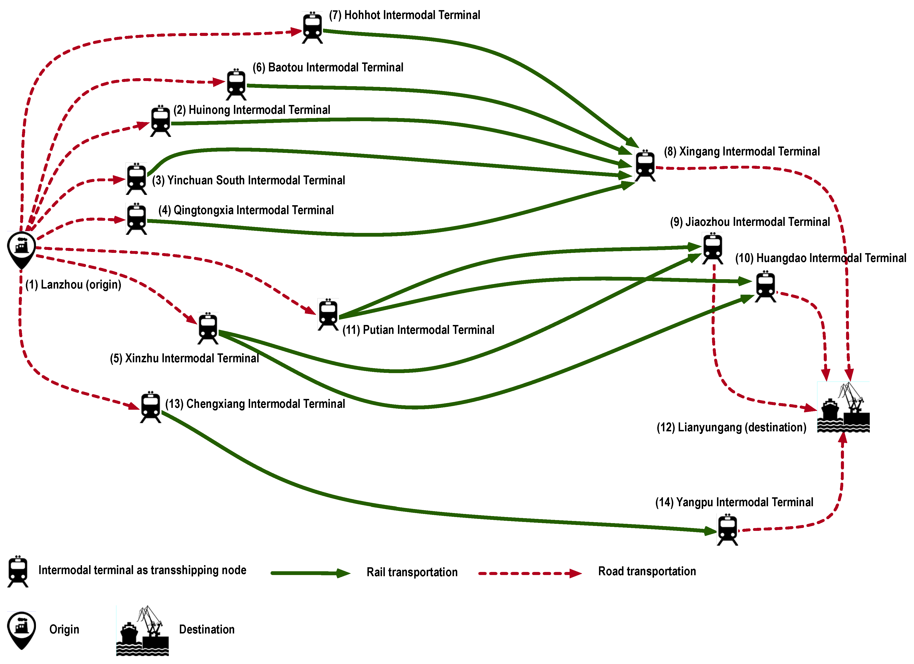
3. Problem Description

3.1. Decision Makings in the Proposed Routing Problem

A green routing problem in a road-rail intermodal hub-and-spoke network was explored in this study. There were two transportation modes in the transportation network, i.e., scheduled rail services and flexible road services. The proposed routing was more than just planning physical distribution routes for the containers of the transportation orders. Based on the explanation given in Section 1, it was a combination and integration of the following decisions that the intermodal operator should be faced with simultaneously, which is illustrated by Figure 1:

(1) Time window selection decision: This decision aims to select time windows for the pickup and delivery service of each transportation and accordingly plan a suitable pickup start time in order to realize on-time services of the entire transportation process. This decision is oriented on the multiple pickup and delivery time windows proposed by the shippers and receivers.

(2) Distribution route design decision: This decision focuses on selecting transshipping nodes (i.e., intermodal terminals) and road/rail services that connect the nodes to design a distribution route for each transportation order. This is the foundational decision in the routing problem, regardless of the specific settings of the problem. This decision significantly influences all the objectives of the road-rail intermodal routing, including economy, timeliness, sustainability and risks.

(3) Truck operations optimization decision: This decision seeks to plan the departure time for trucks of each road service on the planned distribution routes and simultaneously optimize their speeds. This decision is enabled by the flexibility of road services. It deals with the road traffic restrictions and can further lower the costs by improving the transshipping efficiency between road and rail, reduce the carbon dioxide emissions of road services, and achieve on-time deliveries.

Through above-mentioned decisions, this study aimed to optimize the comprehensive performance of the following objectives:

(1) Economic objective: This objective refers to reducing the total costs for accomplishing the container transportation of all the transportation orders served by the intermodal operator and is the most important objective concerned by the transportation buyers when choosing transportation services provided by intermodal operators [9,10].

(2) Timeliness objective: This objective means to realize the on-time road-rail intermodal transportation by using hard time windows to ensure the timeliness of both pickup and delivery services that are at the beginning and end of the transportation process, respectively. This objective reflects the pickup and delivery at the right time and is closely related to the quality of service of the road-rail intermodal transportation [19], which makes it of high importance from the viewpoint of the customers [10].

(3) Environmental sustainability objective: This objective reduces the carbon dioxide emissions of the transportation system to improve its environmental sustainability. Compared with the economic objective, the customers pay less attention to this objective [10]. However, in this study, the environmental sustainability objective is converted into emission profits or costs under the cap-and-trade policy, and hence contributes considerably to the economic objective. In this case, the environmental sustainability objective is integrated into the economic objective, which significantly enhances its importance.

Besides the above three objectives, this study also considered the road-rail intermodal routing in a fuzzy environment to optimize the following objective:

(4) Risk objective: This objective is achieved by considering capacity and the carbon trading price fuzziness and designing a risk-averse approach to obtain a robust routing plan for the transportation orders. This objective lowers the risks on feasibility and optimality that the routing plan is capacity insufficient or not optimum in the actual transportation.

Triangular and trapezoidal fuzzy numbers are the two widely used forms of fuzzy numbers in fuzzy optimizations. Compared with triangular fuzzy numbers, trapezoidal fuzzy numbers enable the decision making to be more flexible by using an interval to represent the most likely situations that are diverse in the fuzzy environment [26]. A trapezoidal fuzzy number can be easily converted into a triangular one when the upper bound of its most likely estimation interval equals its lower bound, which can be used to represent the fuzzy environment where the most likely situation is deterministic and single. Moreover, the utilization of trapezoidal fuzzy numbers does not increase the complexity of fuzzy optimizations, and meanwhile keeps the simplification and flexibility of fuzzy arithmetic operations. Therefore, considering its advantages, trapezoidal fuzzy numbers are employed to represent the fuzzy parameters. A trapezoidal fuzzy parameter (e.g., $\tilde{\vartheta }=\left({\vartheta }_1, {\vartheta }_2, {\vartheta }_3, {\vartheta }_4\right)$), is represented by four prominent points, including minimum estimation value (${\vartheta }_1$), lower bound (${\vartheta }_2$) and upper bound (${\vartheta }_3$) of the most likely estimation interval and maximum estimation value (${\vartheta }_4$) [64]. The fuzzy membership function of $\tilde{\vartheta }$ is presented by Figure 2.

Above all, the consideration of these objectives indicates that the proposed routing is customer centric, since these objectives fully reflect the customer demands [45,58]. The objective setting of the proposed routing corresponds to the goal of the modern transportation industry that is providing customers with the best transportation services. In the routing modeling, the economic and environmental sustainability objectives are integrated together and formulated as the optimization objective of the model, while the timeliness objective is expressed by the hard time window constraint and the risk objective is enhanced by the risk-averse modeling. These objectives may not reach optimum simultaneously, which means that improving an objective could harm others. In this case, the intermodal operator needs to make tradeoffs among them with reference to the customers’ preferences.

3.2. Modeling of the Coordination between Road and Rail in the Transshipment

The coordination between road and rail that is realized by the transshipment process is the essence of the proposed routing problem. The coordination is achieved by the combination of the distribution route design and truck operations optimization. In the transportation system, road services are flexible and carried out by truck fleets [65], while rail services should follow prescribed schedules and refer to container block trains [51]. The schedules are fixed and cannot be changed by the routing. Therefore, the coordination between the two transportation modes through the routing should match the rail schedules, which is the key to ensure that the routing optimization is applicable in practice.

According to Sun et al. [9], the schedule of a rail service regulates the container block train’s arrival time, departure time and service time window at each node on the fixed route and running period. The service time window is an interval that takes the start time and cutoff time of the loading/unloading operation of a container block train at a node as its lower and upper bounds. According to the schedule, a container block train cannot start its loading/unloading operation immediately when it arrives at a node at its scheduled arrival time. It should wait until the lower bound of its service time window and can then start to load/unload containers, and its loading/unloading operation should be immediately terminated at the upper bound of the service time window. After loading, it departs from the node at the scheduled departure time. According to the above discussed regulations, it is clear that rail schedules restrict the coordination (i.e., the transshipment process) through the scheduled (fixed) service time windows.

In the transshipment from road to rail, the containers successively go through the arrival, unloading, waiting (this process does not always exist) and loading processes. Suppose that the selected rail service at a transshipping node yields a service time window $\left[t_L, t_U\right]$, the containers arrive at this node at $t_1$ and are unloaded from the road service at $t_2$, and the selected rail service uses $∆t$ to load the containers. $t_2$ determines whether there is a waiting process in the transshipment. The waiting process exists only when $t_2<t_L$ and the waiting period of the containers is $t_L-t_2$. However, there is no need to wait when $t_2\ge t_L$. In this case, the containers that are unloaded from road can immediately get loaded on rail. In general, a single equation, i.e., $\max \left\{0, t_L-t_2\right\}$, can be used to model the waiting period of the containers in the above two scenarios. Due to an inventory period $\theta$ provided by intermodal terminals that is free, the charged inventory period in the transshipment is $\max \left\{0, t_L-t_2-\theta \right\}$. The distribution route design and truck operations optimization should satisfy Equation (1) to ensure that the transshipment is accomplished before the upper bound of the service time window, so that road and rail can be coordinated by transshipment successfully.

$$\begin{array}{c}\underbrace{\begin{array}{c}\underbrace{t_2}\\ \mathrm{arrival} \mathrm{and} \mathrm{unloading}\end{array}\begin{array}{c}\underbrace{+\max \left\{0, t_L-t_2\right\}}\\ \mathrm{waiting}\end{array}\begin{array}{c}\underbrace{+∆t}\\ \mathrm{loading}\end{array}}\le t_U\\ \mathrm{transshipment} \mathrm{from} \mathrm{road} \mathrm{to} \mathrm{rail}\end{array}$$

(1)

In the transshipment from rail to road, suppose that the rail service uses $∆t^{\prime }$ to unload the containers and loading the containers on road takes $∆t^{″}$. After arriving at the node along with the container block train at its scheduled arrival time, the containers should wait until $t_L$ and then unloaded from the train at $t_L+∆t^{\prime }$. Then, the truck operations optimization decision should determine $t^{*}$, that is the loading start time for the road service. $t^{*}$ should satisfy $t^{*}\ge t_L+∆t^{\prime }$, and $t^{*}+∆t^{″}$, that is the truck departure time should follow the road traffic restrictions and time window constraints. In this transshipment, the waiting period of the containers is $t^{*}-\left(t_L+∆t^{\prime }\right)$ and the corresponding charged inventory period is as $\max \left\{0, t^{*}-\left(t_L+∆t^{\prime }\right)-\theta \right\}$.

3.3. Modeling of the Speed-Dependent Carbon Dioxide Emissions for Road Services

This study aimed to optimize truck speed to further reduce the carbon dioxide emitted by road services. Discrete travel speed options [30] are employed in the truck operations optimization decision making. Lower and upper speed limits are considered when setting speed options for road services. The road-rail intermodal transportation is assumed to use heavy duty trucks whose weights range from 32 to 40 tonnes as road services to carry TEU containers. Moreover, heavy duty trucks are assumed to run on roads with no slope [66]. Based on these assumptions, this study utilized the methodology for calculating transport emissions and energy consumption (MEET), a widely used method proposed by the European Commission [67], to build the speed-dependent rate of carbon dioxide emissions for a truck. MEET suggests using Equation (2) to calculate the emission rate for an unloaded truck.

$$e_0=\left({\kappa }_1+{\kappa }_2·v+{\kappa }_3·v^2+{\kappa }_4·v^3+\frac{{\kappa }_5}{v}+\frac{{\kappa }_6}{v^2}+\frac{{\kappa }_7}{v^3}\right)·{10}^{-3}$$

(2)

where $e_0$ is the emission rate in kg/km for an unloaded truck on a road with a zero gradient, $v$ is the speed in km/h of the truck, κ₁ is a constant, and ${\kappa }_{2,3, \dots ,7}$ are coefficients. When a truck is loaded, MEET adds a load correction factor function shown as Equation (3) to $e_0$ and thereby formulates Equation (4) to calculate the emission rate for a loaded truck:

$$\sigma ={\kappa }_8+{\kappa }_9·\chi +{\kappa }_{10}·{\chi }^2+{\kappa }_{11}·{\chi }^3+{\kappa }_{12}·v+{\kappa }_{13}·v^2+{\kappa }_{14}·v^3+\frac{{\kappa }_{15}}{v}$$

(3)

$$e=e_0·\sigma$$

(4)

where $\sigma$ is the load correction factor, $e$ is the emission rate in kg/km for a loaded truck, χ is the gradient of the road, κ₈ is a constant, and ${\kappa }_{9,10, \dots ,15}$ are coefficients. According to the values of ${\kappa }_{1,2, \dots ,15}$ recommended by MEET, the emission rate for a loaded truck can be calculated by Equation (5). A heavy-duty truck carries a TEU container. Therefore, Equation (5) can be used to formulate the speed-dependent rate of carbon dioxide emissions in kg/TEU/km for road services.

$$e=\left(1576-17.6·v+0.00117·v^3+\frac{36067}{v^2}\right)·\left(1.43-\frac{0.916}{v}\right)·{10}^{-3}$$

(5)

3.4. Proposing of the Methodology

This study planned to establish an optimization model for a road-rail intermodal routing problem with descriptions presented in Section 3.1, Section 3.2 and Section 3.3. First of all, the distribution route design, time window section and truck operations optimization integrated by the routing were all associated with binary and non-negative continuous decision variables. Secondly, the proposed routing problem was formulated in a fuzzy environment where the carbon trading price rate and capacity are fuzzy parameters. Consequently, this study aimed to establish a fuzzy mixed integer nonlinear programming model to optimize the problem under the consideration of the high complexity of the problem (see Section 4.1).

The use of mathematical programming software to implement installed exact solution algorithms has been widely acknowledged to be an effective method in the optimizations. However, due to the nonlinearity and fuzziness, this method cannot be straightforwardly used to solve the proposed model. Therefore, to make the problem solvable, this study first used the linearization technique to reformulate the fuzzy nonlinear model to obtain its equivalent linear form (see Section 4.2). Then, this study used a robust possibilistic programming approach to deal with the fuzzy linear optimization model to generate its crisp reformulation (see Section 5). After the model processing, the problem was solved by using mathematical programming software (LINGO optimizer is used in this study) to implement the exact solution algorithm (Branch-and-Bound Algorithm is used in this study) to generate the solutions.

4. Proposed Green Road-Rail Intermodal Routing Model

All the symbols that are used to define the indices, sets, parameters and variables of the proposed routing model are listed in

Table 1. Notation for the model.

Symbols representing the transportation orders
$K$	Transportation order set.
$k$	Transportation order index, and $k\in K$.
$q_k$	Demand of containers in TEU of transportation order k.
${\tau }_k^{-}$	Index of the origin of transportation order k.
${\tau }_k^{+}$	Index of the destination of transportation order k.
$P_k$	Pickup time window set of transportation order k.
$p$	Pickup time window index of transportation order k, and $p\in P_k$.
$\left[a_p^{k-},a_p^{k+}\right]$	Pickup time window p of transportation order k.
$G_k$	Delivery time window set of transportation order k.
$g$	Delivery time window index of transportation order k, and $g\in G_k$.
$\left[b_g^{k-},b_g^{k+}\right]$	Delivery time window g of transportation order k.
Symbols representing the road-rail intermodal network
$N$	Node set in the network.
$h, i, j$	Node indices, and $h, i, j\in N$.
${\mathsf{\Gamma }}_i^{-}$	Predecessor node set to node i, and ${\mathsf{\Gamma }}_i^{-}\subseteq N$.
${\mathsf{\Gamma }}_i^{+}$	Successor node set to node i, and ${\mathsf{\Gamma }}_i^{+}\subseteq N$.
$A$	Directed arc set in the network.
$\left(i, j\right)$	Directed arc from node i to node j, and $\left(i, j\right)\in A$.
$S$	Transportation service set in the network.
${\mathsf{\Psi }}_{ij}$	Rail service set on arc (i, j) in the network.
${\mathsf{\Omega }}_{ij}$	Road service set on arc (i, j) in the network.
$S_{ij}$	Transportation service set on arc (i, j) in the network, $S_{ij}={\mathsf{\Psi }}_{ij}\cup {\mathsf{\Omega }}_{ij}$ and $S_{ij}\subseteq S$.
$r, s$	Transportation service indices in the network, and $r, s\in S$.
$M_{ijs}$	Discrete travel speed option set of road service s on arc (i, j).
$m$	Travel speed option index, and $m\in M_{ijs}$.
$v_{ijs}^m$	Speed in km/h of option m of road service s on arc (i, j).
$F_{ijs}$	Time interval set that the trucks of road service s on arc (i, j) are allowed to depart from node i.
$f$	Time interval index, and $f\in F_{ijs}$.
$\left({\eta }_{ijs}^{f-}, {\eta }_{ijs}^{f+}\right)$	Allowable departure time interval f for road service s on arc (i, j) under road traffic restrictions.
$d_{ijs}$	Travel distance in km of transportation service s on arc (i, j).
$t_i^s$	Separate loading and unloading time in h/TEU of transportation service s at node i.
$\left[{\phi }_i^{s-},{\phi }_i^{s+}\right]$	Fixed loading and unloading service time window from service start time ${\phi }_i^{s-}$ to service cutoff time ${\phi }_i^{s+}$ of rail service s at node i.
${\tilde{\xi }}_{ijs}$	Fuzzy capacity in TEU of rail service s on arc (i, j), and ${\tilde{\xi }}_{ijs}=\left({\xi }_{ijs}^1, {\xi }_{ijs}^2, {\xi }_{ijs}^3, {\xi }_{ijs}^4\right)$.
Symbols representing the costs and carbon dioxide emissions
$c_1^{\mathrm{rail}}$	Rail travel cost rate in Chinese Yuan (CNY)/TEU.
$c_2^{\mathrm{rail}}$	Rail travel cost rate in CNY/TEU/km.
$c_3^{\mathrm{rail}}$	Inventory cost rate in CNY/TEU/h when containers need to be stored at intermodal terminals.
$\theta$	Inventory period in h that is free of charge at intermodal terminals.
$c^{\mathrm{road}}$	Road travel cost rate in CNY/TEU/km.
$c_s$	Separate loading and unloading cost rate in CNY/TEU of transportation service s.
${\tilde{c}}^{\mathrm{trade}}$	Fuzzy carbon trading price rate in CNY/kg under cap-and-trade policy, and ${\tilde{c}}^{\mathrm{trade}}=\left(c_1^{\mathrm{trade}}, c_2^{\mathrm{trade}}, c_3^{\mathrm{trade}}, c_4^{\mathrm{trade}}\right)$
$cap$	Emission cap in kg for carbon dioxide under cap-and-trade policy.
$e_{ijs}^{\mathrm{rail}}$	Rate of carbon dioxide emissions in kg/TEU/km of rail service s on arc (i, j).
$e_{ijsm}^{\mathrm{road}}$	Rate of carbon dioxide emissions in kg/TEU/km of road service s on arc (i, j) when its truck speed is $v_{ijs}^m$.
Symbol representing the auxiliary parameter
$\varpi$	A predefined sufficient large number.
Symbols representing the variables
$x_{ijs}^k$	0-1 binary decision variable. $x_{ijs}^k=1$ if transportation service s on arc (i, j) is used by the distribution route of transportation order k; $x_{ijs}^k=0$ otherwise.
$w_{ijsf}^k$	0-1 binary decision variable. $w_{ijsf}^k=1$ if the containers of transportation order k depart from node i within time interval f by road service s on arc (i, j); $w_{ijsf}^k=0$ otherwise.
$u_{ijsm}^k$	0-1 binary decision variable. $u_{ijsm}^k=1$ if road service s on arc (i, j) uses travel speed option m to transport the containers of transportation order k; $u_{ijsm}^k=1$ otherwise.
${\rho }_p^k$	0-1 binary decision variable. ${\rho }_p^k=1$ if pickup time window p of transportation order k is selected; ${\rho }_p^k=0$ otherwise.
${ϵ}_g^k$	0-1 binary decision variable. ${ϵ}_g^k=1$ if delivery time window g of transportation order k is selected; ${ϵ}_g^k=0$ otherwise.
${\lambda }_i^k$	Non-negative continuous decision variable denoting the planned time when the containers of transportation order k start to be loaded on trucks at node i before departure.
$l_{ijs}^k$	Non-negative integer variable denoting the day in the planning horizon when the containers of transportation order k depart from node i by road service s on arc (i, j).
$y_i^k$	Non-negative continuous variable denoting the time when the containers of transportation order k arrive at node i and get unloaded from rail or road.
$z_{ijs}^k$	Non-negative continuous variable denoting the waiting period in h of the containers of transportation order k at node i before being transported by rail service s on arc (i, j).
${\pi }_{ijs}^k$	Non-negative continuous variable denoting the charged inventory period in h of the containers of transportation order k at node i before being transported by transportation service s on arc (i, j).

. Accordingly, a fuzzy mixed integer nonlinear programming model and its equivalent linear representation were proposed in the following sections to formulate the problem.

4.1. Optimization Model

The optimization objective of the proposed routing model is as Equation (6). It aims at minimizing the total costs for accomplishing the container transportation of all the transportation orders.

$$\begin{array}{c}\mathrm{minimize} {\displaystyle {\displaystyle \sum }_{k\in K}}{\displaystyle {\displaystyle \sum }_{\left(i,j\right)\in A}}\left[{\displaystyle {\displaystyle \sum }_{s\in {\mathsf{\Psi }}_{ij}}}\left(c_1^{\mathrm{rail}}+c_2^{\mathrm{rail}}·d_{ijs}\right)·q_k·x_{ijs}^k+{\displaystyle {\displaystyle \sum }_{s\in {\mathsf{\Omega }}_{ij}}}{c}^{\mathrm{road}}·d_{ijs}·q_k·x_{ijs}^k\right]\\ +{\displaystyle {\displaystyle \sum }_{k\in K}}{\displaystyle {\displaystyle \sum }_{i\in N}}\left({\displaystyle {\displaystyle \sum }_{h\in {\mathsf{\Gamma }}_i^{-}}}{\displaystyle {\displaystyle \sum }_{r\in S_{hi}}}{c}_r·q_k·x_{hir}^k+{\displaystyle {\displaystyle \sum }_{j\in {\mathsf{\Gamma }}_i^{+}}}{\displaystyle {\displaystyle \sum }_{s\in S_{ij}}}{c}_s·q_k·x_{ijs}^k\right)\\ \begin{array}{c}+{\displaystyle {\displaystyle \sum }_{k\in K}}{\displaystyle {\displaystyle \sum }_{\left(i,j\right)\in A}}{\displaystyle {\displaystyle \sum }_{s\in S_{ij}}}{c}_3^{\mathrm{rail}}·{\pi }_{ijs}^k·q_k\\ +{\tilde{c}}^{\mathrm{trade}}·\left[{\displaystyle {\displaystyle \sum }_{k\in K}}{\displaystyle {\displaystyle \sum }_{\left(i,j\right)\in A}}\left({\displaystyle {\displaystyle \sum }_{s\in {\mathsf{\Psi }}_{ij}}}{e}_{ijs}^{\mathrm{rail}}·d_{ijs}·q_k·x_{ijs}^k+{\displaystyle {\displaystyle \sum }_{s\in {\mathsf{\Omega }}_{ij}}}{\displaystyle {\displaystyle \sum }_{m\in M_{ijs}}}{e}_{ijsm}^{\mathrm{road}}·d_{ijs}·q_k·u_{ijsm}^k\right)-cap\right]\end{array}\end{array}$$

(6)

As indicated by Equation (6), the objectives are achieved by reducing the transportation costs directly related to the road-rail intermodal transportation activities (i.e., the first three terms in the optimization objective that respectively represent the travel costs, loading and unloading operation costs and inventory costs) and lowering carbon dioxide emissions that can either cut down on the emission costs or improve the emission profits under the cap-and-trade policy (i.e., the last term in the optimization objective). Especially, the first term in Equation (6) indicates that the travel costs of rail and road services have different structures in the Chinese scenario, and the structures are regulated by governmental administrations [9]. According to the regulations, the travel costs of a rail service are formulated by two cost rates that are separately related to the demand and turnover accomplished by the rail service on the arc where it runs. However, the formulation of the road travel costs is simpler and is determined by a single cost rate related to the turnover that the road service accomplishes.

In Equation (6), the emissions of road services are dependent on their truck speeds. Based on MEET introduced in Section 3, the emissions are given by Equation (7).

$$e_{ijsm}^{\mathrm{road}}=\left(1576-17.6·v_{ijs}^m+0.00117·v_{ijs}^m{}^3+\frac{36067}{v_{ijs}^m{}^2}\right)·\left(1.43-\frac{0.916}{v_{ijs}^m}\right)·{10}^{-3}$$

(7)

The constraint set on the proposed routing model includes the following equations:

$$\begin{array}{cc}{\displaystyle {\displaystyle \sum }_{h\in {\mathsf{\Gamma }}_i^{-}}}{\displaystyle {\displaystyle \sum }_{r\in S_{hi}}}{x}_{hir}^k-{\displaystyle {\displaystyle \sum }_{j\in {\mathsf{\Gamma }}_i^{+}}}{\displaystyle {\displaystyle \sum }_{s\in S_{ij}}}{x}_{ijs}^k=\{\begin{array}{cc}-1& i={\tau }_k^{-}\\ 0& \forall i=N\backslash \left\{{\tau }_k^{-}, {\tau }_k^{+}\right\}\\ 1& i={\tau }_k^{+}\end{array}& \forall k\in K\end{array}$$

(8)

Equation (8) is the flow equilibrium constraint. It regulates the relationships between the outbound and inbound container flows of the origins, transshipping nodes, and destinations. It ensures that a distribution route is assigned to each transportation order by the routing to accomplish their origin-to-destination transportation.

$$\begin{array}{cc}{\displaystyle {\displaystyle \sum }_{s\in S_{ij}}}{x}_{ijs}^k\le 1& \begin{array}{cc}\forall k\in K& \forall \left(i, j\right)\in A\end{array}\end{array}$$

(9)

Equation (9) is the unsplittable transportation order constraint. It allows that the transportation of the containers of a transportation order can only use a single transportation service on the arc covered on the distribution route, so that the transportation orders are unsplittable during the transportation process.

$$\begin{array}{cc}{\displaystyle {\displaystyle \sum }_{m\in M_{ijs}}}{u}_{ijsm}^k=x_{ijs}^k& \begin{array}{cc}\forall k\in K& \begin{array}{cc}\forall \left(i, j\right)\in A& \forall s\in {\mathsf{\Omega }}_{ij}\end{array}\end{array}\end{array}$$

(10)

Equation (10) is the truck speed selection constraint for road services. It represents that when a road service is selected by the routing to transport the containers, its trucks should select a travel speed.

$$\begin{array}{cc}{\displaystyle {\displaystyle \sum }_{f\in F_{ijs}}}{w}_{ijsf}^k=x_{ijs}^k& \begin{array}{cc}\forall k\in K& \begin{array}{cc}\forall \left(i, j\right)\in A& \forall s\in {\mathsf{\Omega }}_{ij}\end{array}\end{array}\end{array}$$

(11)

Equation (11) is the allowable departure time interval selection constraint for road services under traffic restrictions. It means that the trucks of a road service on the distribution route that is planned for a transportation order should select an allowable departure time interval to plan their departure time from the node, so that the road service operations follow the traffic restrictions.

$$\begin{array}{cc}{l}_{ijs}^k\le \frac{{\lambda }_i^k+t_i^s·q_k}{24}+1& \begin{array}{cc}\forall k\in K& \begin{array}{cc}\forall \left(i, j\right)\in A& \forall s\in {\mathsf{\Omega }}_{ij}\end{array}\end{array}\end{array}$$

(12)

$$\begin{array}{cc}{l}_{ijs}^k>\frac{{\lambda }_i^k+t_i^s·q_k}{24}& \begin{array}{cc}\forall k\in K& \begin{array}{cc}\forall \left(i, j\right)\in A& \forall s\in {\mathsf{\Omega }}_{ij}\end{array}\end{array}\end{array}$$

(13)

$$\begin{array}{cc}{\lambda }_i^k+t_i^s·q_k-24·\left(l_{ijs}^k-1\right)>{\eta }_{ijs}^{f-}+\varpi ·\left(w_{ijsf}^k-1\right)& \begin{array}{cc}\forall k\in K& \begin{array}{cc}\forall \left(i, j\right)\in A& \begin{array}{cc}\forall s\in {\mathsf{\Omega }}_{ij}& \forall f\in F_{ijs}\end{array}\end{array}\end{array}\end{array}$$

(14)

$$\begin{array}{cc}{\lambda }_i^k+t_i^s·q_k-24·\left(l_{ijs}^k-1\right)<{\eta }_{ijs}^{f+}+\varpi ·\left(1-w_{ijsf}^k\right)& \begin{array}{cc}\forall k\in K& \begin{array}{cc}\forall \left(i, j\right)\in A& \begin{array}{cc}\forall s\in {\mathsf{\Omega }}_{ij}& \forall f\in F_{ijs}\end{array}\end{array}\end{array}\end{array}$$

(15)

Equations (12)–(15) are the truck departure time constraints. It ensures that the trucks of a road service that are used to transport the containers depart from the node within the selected allowable departure time interval. In these equations, Equations (12) and (13) determine a non-negative integer variable $l_{ijs}^k$, i.e., the day when the trucks of the road service depart from the node. Then $l_{ijs}^k$ is used to convert ${\lambda }_i^k+t_i^s·q_k$, i.e., the planned departure time of the trucks of the road service, into 0–24 that is the time interval of a day. After processing, the converted departure time should satisfy the traffic restrictions, which is indicated by Equations (14) and (15).

$$\begin{array}{cc}{\displaystyle {\displaystyle \sum }_{p\in P_k}}{\rho }_p^k=1& \forall k\in K\end{array}$$

(16)

$$\begin{array}{cc}{\displaystyle {\displaystyle \sum }_{g\in G_k}}{ϵ}_g^k=1& \forall k\in K\end{array}$$

(17)

Equations (16) and (17) are the time window selection constraints. It stresses that the road-rail intermodal routing for each transportation order should select only one pickup time window and one delivery time window from the multiple choices.

$$\begin{array}{cc}{\lambda }_{{\tau }_k^{-}}^k\ge a_p^{k-}+\varpi ·\left({\rho }_p^k-1\right)& \begin{array}{cc}\forall k\in K& \forall p\in P_k\end{array}\end{array}$$

(18)

$$\begin{array}{cc}{\lambda }_{{\tau }_k^{-}}^k\le a_p^{k+}+\varpi ·\left(1-{\rho }_p^k\right)& \begin{array}{cc}\forall k\in K& \forall p\in P_k\end{array}\end{array}$$

(19)

$$\begin{array}{cc}{y}_{{\tau }_k^{+}}^k\ge b_g^{k-}+\varpi ·\left({ϵ}_g^k-1\right)& \begin{array}{cc}\forall k\in K& \forall g\in G_k\end{array}\end{array}$$

(20)

$$\begin{array}{cc}{y}_{{\tau }_k^{+}}^k\le b_g^{k-}+\varpi ·\left(1-{ϵ}_g^k\right)& \begin{array}{cc}\forall k\in K& \forall g\in G_k\end{array}\end{array}$$

(21)

Equations (18)–(21) are the hard time window constraints. The container transportation for each transportation order begins at a planned pickup start time (i.e., the loading start time of the containers at the origin) and ends at the delivery accomplishment time (i.e., the unloading accomplishment time of containers at the destination). Both pickup start time and delivery accomplishment time of a transportation order should fall into respective time windows.

$$\begin{array}{cc}{\lambda }_i^k\ge y_i^k& \begin{array}{cc}\forall k\in K& \forall i\in {\mathsf{\Gamma }}_{{\tau }_k^{+}}^{-}\backslash \left\{{\tau }_k^{-}\right\}\end{array}\end{array}$$

(22)

Equation (22) is the loading start time constraints. It clarifies that the loading start time of the containers of a transportation order should not be earlier than the time when these containers complete the predecessor unloading operation.

$$\begin{array}{cc}{y}_{{\tau }_k^{-}}^k={\lambda }_{{\tau }_k^{-}}^k& \forall k\in K\end{array}$$

(23)

$$\begin{array}{cc}\left({\lambda }_i^k+t_i^s·q_k+{\displaystyle {\displaystyle \sum }_{m\in M_{ijs}}}{u}_{ijsm}^k·\frac{d_{ijs}}{v_{ijs}^m}+t_j^s·q_k-y_j^k\right)·x_{ijs}^k=0& \begin{array}{cc}\forall k\in K& \begin{array}{cc}\forall \left(i, j\right)\in A& \forall s\in {\mathsf{\Omega }}_{ij}\end{array}\end{array}\end{array}$$

(24)

$$\begin{array}{cc}\left({\phi }_j^{s-}+t_j^s·q_k-y_j^k\right)·x_{ijs}^k=0& \begin{array}{cc}\forall k\in K& \begin{array}{cc}\forall \left(i, j\right)\in A& \forall s\in {\Psi }_{ij}\end{array}\end{array}\end{array}$$

(25)

Equations (23)–(25) are the variable computation constraints that determine the time when the containers of a transportation order arrive and are unloaded at the node covered on the distribution route. Particularly, Equation (23) assumes that the time when the containers arrive and are unloaded at the origin equals the planned pickup start time for them. This assumption initializes a series of computations to obtain the above-mentioned time variables. Equations (24) and (25) separately refer to the situations where the containers are transported by road and rail.

$$\begin{array}{cc}\left(z_{ijs}^k-\max \left\{{\phi }_i^{s-}-y_i^k, 0\right\}\right)·x_{ijs}^k=0& \begin{array}{cc}\forall k\in K& \begin{array}{cc}\forall \left(i, j\right)\in A& \forall s\in {\mathsf{\Psi }}_{ij}\end{array}\end{array}\end{array}$$

(26)

$$\begin{array}{cc}{\pi }_{ijs}^k=\max \left\{{\lambda }_i^k-y_i^k-\theta , 0\right\}& \begin{array}{cc}\forall k\in K& \begin{array}{cc}\forall \left(i, j\right)\in A& \forall s\in {\mathsf{\Omega }}_{ij}\end{array}\end{array}\end{array}$$

(27)

$$\begin{array}{cc}{\pi }_{ijs}^k=\max \left\{z_{ijs}^k-\theta , 0\right\}& \begin{array}{cc}\forall k\in K& \begin{array}{cc}\forall \left(i, j\right)\in A& \forall s\in {\mathsf{\Psi }}_{ij}\end{array}\end{array}\end{array}$$

(28)

Equations (26)–(28) are the variable computation constraints. The first equation gives the waiting period of the containers of a transportation order during the transshipment from road to rail. The second and third present the computation of the charged inventory period by considering a free-of-charge period at the intermodal terminals, and this variable directly contributes to the optimization objective.

$$\begin{array}{cc}{y}_i^k+z_{ijs}^k+t_i^s·q_k\le {\phi }_i^{s+}·x_{ijs}^k+\varpi ·\left(1-x_{ijs}^k\right)& \begin{array}{cc}\forall k\in K& \begin{array}{cc}\forall \left(i, j\right)\in A& \forall s\in {\mathsf{\Psi }}_{ij}\end{array}\end{array}\end{array}$$

(29)

Equation (29) is the service time constraint of rail services. It enforces that the containers should be loaded on the selected rail service no later than the service cutoff time regulated by its schedule.

$$\begin{array}{cc}{\displaystyle {\displaystyle \sum }_{k\in K}}{q}_k·x_{ijs}^k\le {\tilde{\xi }}_{ijs}& \begin{array}{cc}\forall \left(i, j\right)\in A& \forall s\in {\mathsf{\Psi }}_{ij}\end{array}\end{array}$$

(30)

Equation (30) is the fuzzy capacity constraint. It ensures that the containers loaded on to a rail service should not exceed its the capacity that is formulated as a trapezoidal fuzzy parameter.

$$\begin{array}{cc}{x}_{ijs}^k\in \left\{0, 1\right\}& \begin{array}{cc}\forall k\in K& \begin{array}{cc}\forall \left(i, j\right)\in A& \forall s\in S_{ij}\end{array}\end{array}\end{array}$$

(31)

$$\begin{array}{cc}{w}_{ijsf}^k\in \left\{0, 1\right\}& \begin{array}{cc}\forall k\in K& \begin{array}{cc}\forall \left(i, j\right)\in A& \begin{array}{cc}\forall s\in {\mathsf{\Omega }}_{ij}& \forall f\in F_{ijs}\end{array}\end{array}\end{array}\end{array}$$

(32)

$$\begin{array}{cc}{u}_{ijsm}^k\in \left\{0, 1\right\}& \begin{array}{cc}\forall k\in K& \begin{array}{cc}\forall \left(i, j\right)\in A& \begin{array}{cc}\forall s\in {\mathsf{\Omega }}_{ij}& \forall m\in M_{ijs}\end{array}\end{array}\end{array}\end{array}$$

(33)

$$\begin{array}{cc}{\rho }_p^k\in \left\{0, 1\right\}& \begin{array}{cc}\forall k\in K& \forall p\in P_k\end{array}\end{array}$$

(34)

$$\begin{array}{cc}{ϵ}_g^k\in \left\{0, 1\right\}& \begin{array}{cc}\forall k\in K& \forall g\in G_k\end{array}\end{array}$$

(35)

$$\begin{array}{cc}{\lambda }_i^k\ge 0& \begin{array}{cc}\forall k\in K& \forall i\in {\mathsf{\Gamma }}_{{\tau }_k^{+}}^{-}\cup \left\{{\tau }_k^{-}\right\}\end{array}\end{array}$$

(36)

$$\begin{array}{cc}{l}_{ijs}^k\ge 0 \mathrm{and} \mathrm{integer}& \begin{array}{cc}\forall k\in K& \begin{array}{cc}\forall \left(i, j\right)\in A& \forall s\in {\Omega }_{ij}\end{array}\end{array}\end{array}$$

(37)

$$\begin{array}{cc}{y}_i^k\ge 0& \begin{array}{cc}\forall k\in K& \forall i\in N\end{array}\end{array}$$

(38)

$$\begin{array}{cc}{z}_{ijs}^k\ge 0& \begin{array}{cc}\forall k\in K& \begin{array}{cc}\forall \left(i, j\right)\in A& \forall s\in {\mathsf{\Psi }}_{ij}\end{array}\end{array}\end{array}$$

(39)

$$\begin{array}{cc}{\pi }_{ijs}^k\ge 0& \begin{array}{cc}\forall k\in K& \begin{array}{cc}\forall \left(i, j\right)\in A& \forall s\in S_{ij}\end{array}\end{array}\end{array}$$

(40)

Equations (31)–(40) are the variable domain constraints.

4.2. Model Linearization

The proposed model is straightforwardly based on the problem description, which makes its representation easily understandable. However, it is nonlinear because the formulations of Equations (24)–(28) contain either a multiplication of variables or maximum functions containing variables. Considering a large number of constraints and indices in the nonlinear model, finding the optimal solutions to the proposed routing problem has high computational complexity [60,68]. Therefore, this study conducts the model linearization by using the linearization technique developed by the author in previous studies [9,26], which enables the optimization problems to be relatively easy to solve [69].

By introducing the following new constraints to take place of Equations (24)–(28) that are nonlinear, this study presents an equivalent linear reformation for the proposed routing model. Based on the author’s linearization technique, the combinations of Equations (41) and (42) and of Equations (43) and (44) are used to linearize Equations (24) and (25), respectively.

$$\begin{array}{cc}{\lambda }_i^k+t_i^s·q_k+{\displaystyle {\displaystyle \sum }_{m\in M_{ijs}}}{u}_{ijsm}^k·\frac{d_{ijs}}{v_{ijs}^m}+t_j^s·q_k-y_j^k\ge \varpi ·\left(x_{ijs}^k-1\right)& \begin{array}{cc}\forall k\in K& \begin{array}{cc}\forall \left(i, j\right)\in A& \forall s\in {\mathsf{\Omega }}_{ij}\end{array}\end{array}\end{array}$$

(41)

$$\begin{array}{cc}{\lambda }_i^k+t_i^s·q_k+{\displaystyle {\displaystyle \sum }_{m\in M_{ijs}}}{u}_{ijsm}^k·\frac{d_{ijs}}{v_{ijs}^m}+t_j^s·q_k-y_j^k\le \varpi ·\left(1-x_{ijs}^k\right)& \begin{array}{cc}\forall k\in K& \begin{array}{cc}\forall \left(i, j\right)\in A& \forall s\in {\mathsf{\Omega }}_{ij}\end{array}\end{array}\end{array}$$

(42)

$$\begin{array}{cc}{\phi }_j^{s-}+t_j^s·q_k-y_j^k\ge \varpi ·\left(x_{ijs}^k-1\right)& \begin{array}{cc}\forall k\in K& \begin{array}{cc}\forall \left(i, j\right)\in A& \forall s\in {\mathsf{\Psi }}_{ij}\end{array}\end{array}\end{array}$$

(43)

$$\begin{array}{cc}{\phi }_j^{s-}+t_j^s·q_k-y_j^k\le \varpi ·\left(1-x_{ijs}^k\right)& \begin{array}{cc}\forall k\in K& \begin{array}{cc}\forall \left(i, j\right)\in A& \forall s\in {\mathsf{\Psi }}_{ij}\end{array}\end{array}\end{array}$$

(44)

Furthermore, nonlinear Equations (26)–(28) can be linearized by the following equations successively.

$$\begin{array}{cc}{z}_{ijs}^k\ge \left({\phi }_i^{s-}-y_i^k\right)+\varpi ·\left(x_{ijs}^k-1\right)& \begin{array}{cc}\forall k\in K& \begin{array}{cc}\forall \left(i, j\right)\in A& \forall s\in {\mathsf{\Psi }}_{ij}\end{array}\end{array}\end{array}$$

(45)

$$\begin{array}{cc}{\pi }_{ijs}^k\ge \left({\lambda }_i^k-y_i^k-\theta \right)+\varpi ·\left(x_{ijs}^k-1\right)& \begin{array}{cc}\forall k\in K& \begin{array}{cc}\forall \left(i, j\right)\in A& \forall s\in {\mathsf{\Omega }}_{ij}\end{array}\end{array}\end{array}$$

(46)

$$\begin{array}{cc}{\pi }_{ijs}^k\ge z_{ijs}^k-\theta & \begin{array}{cc}\forall k\in K& \begin{array}{cc}\forall \left(i, j\right)\in A& \forall s\in {\mathsf{\Psi }}_{ij}\end{array}\end{array}\end{array}$$

(47)

After the above linearization processing, a fuzzy mixed integer linear programming model is provided to optimize the problem. Its optimization objective is Equation (6) and its constraint set includes Equations (8)–(23) and (29)–(47). Above all, the linear programming model uses equivalent linear reformations to replace the corresponding nonlinear constraints in the initial model proposed in Section 4.1 and Section 4.2. The detailed proofs on the above-mentioned linearization can be found in the author’s previous study [26] that demonstrated their equivalence. Therefore, the linear programming model can obtain the same solutions to the initial nonlinear one when solving the proposed routing problem. Additionally, the equivalent linear programming model is more suitable to be used for the problem solving that adopts exact solution algorithms implemented by mathematical programming software.

Although the model linearization reduces the computational complexity, the problem still cannot be solved due to the existence of imprecise information in both objective functions (i.e., Equations (6)) and constraint (i.e., Equation (30)) of the reformulated model. The fuzziness makes crisp routing schemes unattainable for the intermodal operator. Therefore, this study needed to further deal with the fuzzy linear programming model to generate its crisp form that can then be solved to output crisp solutions.

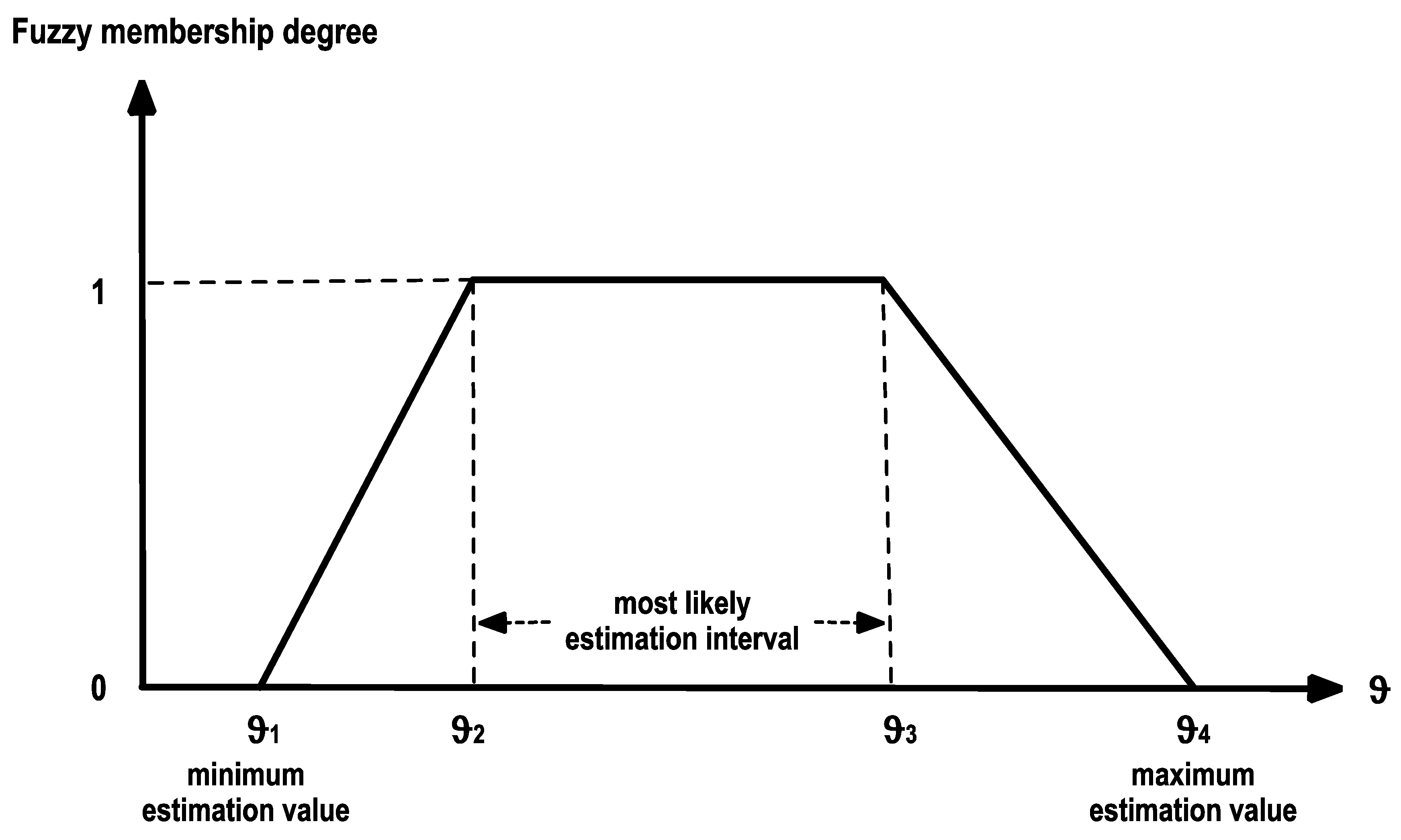
5. Proposed Robust Possibilistic Programming Approach

Fuzzy mathematical programming can be classified into two categories: possibilistic programming and flexible programming. Possibilistic programming is used to address imprecise/ambiguous parameters of objective functions and constraints that are modeled by utilizing available objective data that are not enough in most cases and subjective knowledge/experience of decision makers, while flexible programming aims to handle flexible target values of objectives and constraints [70]. This study considers imprecise parameters (i.e., fuzzy capacities and fuzzy carbon trading price rate) in the proposed routing problem. Therefore, the model in Section 4 belongs to possibilistic programming.

Although possibilistic programming approaches are extensively employed to address the optimization problems under uncertainty, they are incapable of controlling objective function risk and only use average values of imprecise/ambiguous parameters to obtain the optimization results of the problem [71]. To overcome the disadvantages of the possibilistic programming approach, Pishvaee et al. developed the robust possibilistic programming (RPP) approach combining the advantages of possibilistic and robust programming approaches [54]. The RPP provides flexible solutions to different situations of the problem concerned by decision makers and takes the worst case for the objective function into account to cope with risks in real-world applications [72]. According to Pishvaee et al. [54], a robust solution to an optimization problem under uncertainty should both have: (1) feasibility robustness indicating that such a solution should be feasible for all possible values of the uncertain parameters, and (2) optimality robustness meaning that the value of the objective function for such a solution must be close to the optimal value for all possible values of the uncertain parameters. Recently, RPP has been acknowledged by studies on optimization problems under uncertainty and is adopted by this study to process the routing model considering both capacity and the carbon trading price rate uncertainty. Before further dealing with the model after linearization, this study first used $c^{\mathrm{transportation}}$ (see Equation (48)) and $q^{\mathrm{emission}}$ (see Equation (49)) to denote the transportation costs and carbon dioxide emissions in Equation (6), respectively. The objective function can be rewritten as Equation (50).

$$\begin{array}{c}{c}^{\mathrm{transportation}}={\displaystyle {\displaystyle \sum }_{k\in K}}{\displaystyle {\displaystyle \sum }_{\left(i,j\right)\in A}}\left[{\displaystyle {\displaystyle \sum }_{s\in {\mathsf{\Psi }}_{ij}}}\left(c_1^{\mathrm{rail}}+c_2^{\mathrm{rail}}·d_{ijs}\right)·q_k·x_{ijs}^k+{\displaystyle {\displaystyle \sum }_{s\in {\mathsf{\Omega }}_{ij}}}{c}^{\mathrm{road}}·d_{ijs}·q_k·x_{ijs}^k\right]\\ +{\displaystyle {\displaystyle \sum }_{k\in K}}{\displaystyle {\displaystyle \sum }_{i\in N}}\left({\displaystyle {\displaystyle \sum }_{h\in {\mathsf{\Gamma }}_i^{-}}}{\displaystyle {\displaystyle \sum }_{r\in S_{hi}}}{c}_r·q_k·x_{hir}^k+{\displaystyle {\displaystyle \sum }_{j\in {\mathsf{\Gamma }}_i^{+}}}{\displaystyle {\displaystyle \sum }_{s\in S_{ij}}}{c}_s·q_k·x_{ijs}^k\right)\\ +{\displaystyle {\displaystyle \sum }_{k\in K}}{\displaystyle {\displaystyle \sum }_{\left(i,j\right)\in A}}{\displaystyle {\displaystyle \sum }_{s\in S_{ij}}}{c}_3^{\mathrm{rail}}·{\pi }_{ijs}^k·q_k\end{array}$$

(48)

$$q^{\mathrm{emission}}={\displaystyle {\displaystyle \sum }_{k\in K}}{\displaystyle {\displaystyle \sum }_{\left(i,j\right)\in A}}\left({\displaystyle {\displaystyle \sum }_{s\in {\mathsf{\Psi }}_{ij}}}{e}_{ijs}^{\mathrm{rail}}·d_{ijs}·q_k·x_{ijs}^k+{\displaystyle {\displaystyle \sum }_{s\in {\mathsf{\Omega }}_{ij}}}{\displaystyle {\displaystyle \sum }_{m\in M_{ijs}}}{e}_{ijsm}^{\mathrm{road}}·d_{ijs}·q_k·u_{ijsm}^k\right)$$

(49)

$$obj=c^{\mathrm{transportation}}+{\tilde{c}}^{\mathrm{trade}}·\left(q^{\mathrm{emission}}-cap\right)$$

(50)

5.1. Basic Possibilistic Chance-Constrained Programming Model

The basic possibilistic chance-constrained programming (BPCCP) can be used to handle the proposed routing model with fuzzy parameters in both objective function and constraint. The BPCCP adopts the expected value operator that yields the linearity property to deal with the fuzzy objective function [73]. Using this operator, the crisp form of the fuzzy objective is as Equation (51) that means to minimize the average value of the total costs for accomplishing the container transportation of all the transportation orders.

$$\mathrm{minimize} \mathrm{E}\left[obj\right]=\mathrm{minimize} c^{\mathrm{transportation}}+\mathrm{E}\left[{\tilde{c}}^{\mathrm{trade}}\right]·\left(q^{\mathrm{emission}}-cap\right)$$

(51)

According to [74], $\mathrm{E}\left[{\tilde{c}}^{\mathrm{trade}}\right]=\left(c_1^{\mathrm{trade}}+c_2^{\mathrm{trade}}+c_3^{\mathrm{trade}}+c_4^{\mathrm{trade}}\right)/4$. Consequently, the crisp representation of the fuzzy objective of the BPCCP model is shown as Equation (52).

$$\mathrm{minimize} c^{\mathrm{transportation}}+\frac{c_1^{\mathrm{trade}}+c_2^{\mathrm{trade}}+c_3^{\mathrm{trade}}+c_4^{\mathrm{trade}}}{4}·\left(q^{\mathrm{emission}}-cap\right)$$

(52)

Furthermore, the BPCCP uses the necessity measure to handle the constraint with fuzzy parameter. The fuzzy capacity constraint Equation (30) is accordingly converted into a necessity-based chance constraint (see Equation (53)). The use of the necessity measure in the BPCCP shows its pessimistic perspective and appreciates for risk-averse decision makings [75].

$$\begin{array}{cc}\mathrm{Nec}\left\{{\displaystyle {\displaystyle \sum }_{k\in K}}{q}_k·x_{ijs}^k\le {\tilde{\xi }}_{ijs}\right\}\ge {\alpha }^{\prime }& \begin{array}{cc}\forall \left(i, j\right)\in A& \forall s\in {\mathsf{\Psi }}_{ij}\end{array}\end{array}$$

(53)

In Equation (53), ${\alpha }^{\prime }$ is the minimum acceptable confidence level, and there is ${\alpha }^{\prime }\in \left[0, 1.0\right]$. It is an interactive parameter determined by decision makers before solving the problem. This equation means that the necessity that the fuzzy event “${\displaystyle \sum _{k\in K}}{q}_k·x_{ijs}^k\le {\tilde{\xi }}_{ijs}$” holds should not be less than ${\alpha }^{\prime }$.

For a trapezoidal fuzzy number $\tilde{\vartheta }=\left({\vartheta }_1, {\vartheta }_2, {\vartheta }_3, {\vartheta }_4\right)$ and a deterministic number $\vartheta ,$ there is Equation (54) expressing the necessity that $\vartheta$ is not bigger than $\tilde{\vartheta }$, and this equation can be further derived as Equation (55) [76]:

$$\mathrm{Nec}\left\{\vartheta \le \tilde{\vartheta }\right\}=\{\begin{array}{cc}1,& \mathrm{if} \vartheta \le {\vartheta }_1\\ \frac{{\vartheta }_2-\vartheta }{{\vartheta }_2-{\vartheta }_1},& \mathrm{if} {\vartheta }_1\le \vartheta \le {\vartheta }_2\\ 0,& \mathrm{if} \vartheta \ge {\vartheta }_2\end{array}$$

(54)

$$\mathrm{Nec}\left\{\vartheta \le \tilde{\vartheta }\right\}\ge {\alpha }^{\prime } ⟺ \vartheta \le {\alpha }^{\prime }·{\vartheta }_1+\left(1-{\alpha }^{\prime }\right)·{\vartheta }_2$$

(55)

According to Equation (55), Equation (53) equals to Equation (56) that is a crisp linear formulation.

$$\begin{array}{cc}{\displaystyle {\displaystyle \sum }_{k\in K}}{q}_k·x_{ijs}^k\le {\alpha }^{\prime }·{\xi }_{ijs}^1+\left(1-{\alpha }^{\prime }\right)·{\xi }_{ijs}^2& \begin{array}{cc}\forall \left(i, j\right)\in A& \forall s\in {\mathsf{\Psi }}_{ij}\end{array}\end{array}$$

(56)

Above all, the BPCCP model for the proposed routing problem takes Equation (52) as its optimization objective and Equations (8)–(23), (29), (31)–(47) and (56) as its constraints.

5.2. Robust Possibilistic Programming Model

The BPCCP model makes the proposed routing problem crisp and thereby solvable. However, the BPCCP approach cannot cope with the average performance of the objective function well [71]. To overcome this weakness, robust programming that is a risk-averse approach is integrated into the BPCCP approach, which leads to the development of RPP approaches. Based on the BPCCP, Pishvaee et al. [54] first designed several versions of RPP approaches when optimizing a supply chain network design under fuzziness. In their study, the RPP-II approach shows the best performance and has been paid attention by transportation planning problems [77,78]. Using the RPP-II approach to address the fuzzy capacity constraint of the road-rail intermodal routing model also leads into a necessity-based chance constraint Equation (57), which is similar to the establishment of Equation (53).

$$\begin{array}{cc}\mathrm{Nec}\left\{{\displaystyle {\displaystyle \sum }_{k\in K}}{q}_k·x_{ijs}^k\le {\tilde{\xi }}_{ijs}\right\}\ge \alpha & \begin{array}{cc}\forall \left(i, j\right)\in A& \forall s\in {\Psi }_{ij}\end{array}\end{array}$$

(57)

Confidence level $\alpha$ in Equation (57) has the same meaning to confidence level ${\alpha }^{\prime }$ in Equation (53). However, instead of setting ${\alpha }^{\prime }$ as an inactive parameter in the BPCCP model, $\alpha$ in the RPP model is a variable whose domain is restricted by Equation (58) where ${\alpha }_0$ is the lower bound of $\alpha$ that is set by decision makers. Therefore, ${\alpha }_0$ is also an interactive parameter, with ${\alpha }_0\ge 0.5$.

$${\alpha }_0\le \alpha \le 1.0$$

(58)

Based on Equation (55), Equation (57) can be also derived as Equation (59) where $\alpha ·{\xi }_{ijs}^1+\left(1-\alpha \right)·{\xi }_{ijs}^2$ is the chance constraint value of fuzzy capacity ${\tilde{\xi }}_{ijs}$.

$$\begin{array}{cc}{\displaystyle {\displaystyle \sum }_{k\in K}}{q}_k·x_{ijs}^k\le \alpha ·{\xi }_{ijs}^1+\left(1-\alpha \right)·{\xi }_{ijs}^2& \begin{array}{cc}\forall \left(i, j\right)\in A& \forall s\in {\Psi }_{ij}\end{array}\end{array}$$

(59)

The objective of the RPP model for the proposed routing problem in this study is as Equation (60) in which the objective of the BPCCP model is included as the first term.

$$\mathrm{minimize} \mathrm{E}\left[obj\right]+\gamma ·\left(ob{j}_{\max }-\mathrm{E}\left[obj\right]\right)+\delta ·{\displaystyle {\displaystyle \sum }_{\left(i, j\right)\in A}}{\displaystyle {\displaystyle \sum }_{s\in {\mathsf{\Psi }}_{ij}}}\left[\alpha ·{\xi }_{ijs}^1+\left(1-\alpha \right)·{\xi }_{ijs}^2-{\xi }_{ijs}^1\right]$$

(60)

In Equation (60), the first term shows the average performance of the robust optimization on minimizing the expected value of the fuzzy objective of the proposed routing. The second term represents the optimality robustness costs, and optimality robustness minimizes the difference between the maximum possible value ($ob{j}_{\max }$) of the objective function and its expected value. This term provides decision makers with a risk-averse solution. In this term, $ob{j}_{\max }$ is obtained by Equation (61), and $\gamma \in \left[0, 1.0\right]$ is the importance weight of the optimality robustness in comparison with the other two terms.

$$ob{j}_{\max }=c^{\mathrm{transportation}}+c_4^{\mathrm{trade}}·\left(q^{\mathrm{emission}}-cap\right)$$

(61)

The third term in Equation (60) indicates the feasibility robustness costs. Feasibility robustness minimizes the difference between the worst-case value (${\xi }_{ijs}^1$) of the fuzzy capacity and its chance constraint value ($\alpha ·{\xi }_{ijs}^1+\left(1-\alpha \right)·{\xi }_{ijs}^2$). This term determines the value of confidence level $\alpha$ in Equation (59). In this term, δ is the penalty for violating the chance constrai. It is meaningful and calculable based on the damage caused by the violation [79].

Above all, the RPP model for the proposed routing problem takes Equation (60) as its optimization objective and Equations (8)–(23), (29), (31)–(47), (58) and (59) as its constraints.

6. An Empirical Case Study

In this section, a Chinese scenario-oriented empirical case from the author’s previous study [9] was modified to fit into the problem description of this study and then used to implement and evaluate the proposed approaches. In the case study, the intermodal operator serves multiple transportation orders from Lanzhou to Lianyungang by routing their containers within a one-week planning horizon. Based on the locations of Lanzhou, an inland city of the Gansu Province, Northwestern China and Lianyungang, a seaport of the Jiangsu Province, Eastern China, a road-rail intermodal hub-and-spoke network was constructed, as shown in Figure 3, for the container transportation between the origin and destination.

In the transportation network, there were 12 road transportation lines (i.e., expressways) that could be used by pickup and delivery services. Each road transportation line had a truck fleet group. The truck fleet group could be divided into several sub-groups to serve the transportation orders according to the distribution route design. Based on the vehicle speed limits of the expressways in China, the discrete travel speed options in km/h were set at 60, 65, 70, 75, 80, 85, 90, 95, and 100, with a step of 5 km/h. Moreover, the road traffic restrictions were from 19:00 p.m. to 6:00 a.m. [29]. There were 10 rail transportation lines with 10 container block trains running on them periodically. The detailed information of rail and road services is given in Tables S1 and S2 in the supplementary material. The case study considered 10 transportation orders whose containers needed to be transported from Lanzhou to Lianyungang using the road-rail intermodal network shown as Figure 3, and each transportation order had three pickup/delivery time windows, which can be seen in Table S3. The values of the cost and time parameters of transportation services are given in Table S4, in which the costs related to transportation services are regulated by governmental administrations [26], unit unloading and unloading times of rail and road services referred to Resat and Turkay’s study [80], and fuzzy the carbon trading price rate was determined based on Zhang et al.’s article [81].

Before solving the problem, all the data of the parameters related to time in the above-mentioned tables were converted into real numbers. For example, 8:00 on the second day in the planning horizon was converted into 32. Additionally, the same container block train running in different periods was modeled as different rail services [9]. For example, the container block train running from Huinong to Xingang yielded a service time window [5,11] at Huinong in its first period. In the second period, this train was treated as a different rail service with a service time window [53,59] at Huinong.

6.1. Optimization Results

This study used LINGO optimizer on a Lenovo Laptop with Intel Core i5-5200U 2.20 GHz CPU 8 GB RAM using Microsoft Windows 10 operating system to encode the BPCCP and RPP models to optimize the proposed routing problem. LINGO optimizer runs Branch-and-Bound Algorithm to solve the models to obtain the global optimum solutions. The two models contained following interactive parameters that should be determined by decision makers in advance: (1) $cap$ in the two models, (2) ${\alpha }^{\prime }$ in the BPCCP model, and (3) $\gamma$, $\delta$ and ${\alpha }_0$ in the RPP model. In the implementation, these parameters were first set according to

Table 2. Settings of the interactive parameters in the models.

Interactive Parameters	Models	Values
$cap$	BPCCP and RPP	300,000 kg
${\alpha }^{\prime }$	BPCCP	0.6, 0.8, 1.0
$\gamma$	RPP	0.5
$\delta$	RPP	30 CNY/TEU
${\alpha }_0$	RPP	0.5

, and the optimization results are presented in

Table 3. Optimization results of the BPCCP and RPP models.

$$\begin{gathered} \mathbf{BPCCP} \\ {\mathit{\alpha }}^{\prime }\mathbf{=}\mathbf{1.0} \end{gathered}$$	$$\begin{gathered} \mathbf{BPCCP} \\ {\mathit{\alpha }}^{\prime }\mathbf{=}\mathbf{0.8} \end{gathered}$$	$$\begin{gathered} \mathbf{BPCCP} \\ {\mathit{\alpha }}^{\prime }\mathbf{=}\mathbf{0.6} \end{gathered}$$	RPP
Expected Costs (CNY)			Expected Costs (CNY)	Optimality Robustness Costs (CNY)	Feasibility Robustness Costs (CNY)	Total Costs (CNY)
2,477,946	2,478,256	2,471,574	2,466,173	536.6	2385	2,469,095
Running time (s) of LINGO optimizer
22	21	27	56

.

As shown in Table 3, although adding optimality robustness and feasibility robustness into the objective function, the total costs obtained by the RPP model was lower than these of the BPCCP model under different confidence levels. Table 3 finds that the RPP model reduced the expected costs of the routing, which covered the increase of the resulting robustness related costs. Compared with BPCCP model, the RPP model consumed more time to obtain the solution to the problem, since it contained more variables and constraints than the BPCCP model. However, the efficiency of the RPP model was still acceptable. Therefore, the RPP model was more effective to optimize the proposed routing problem under the settings of Table 2.

6.2. Case Analysis

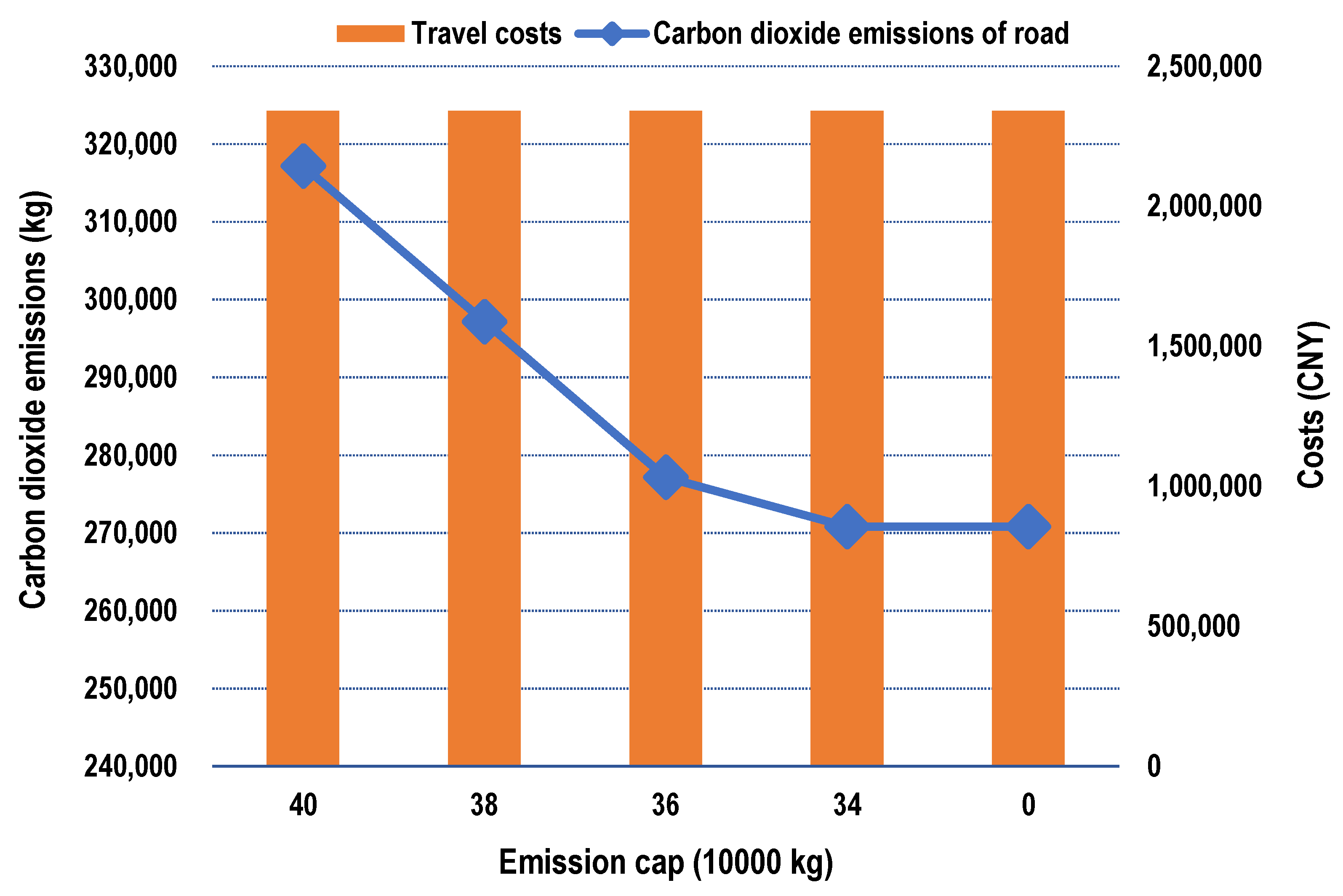
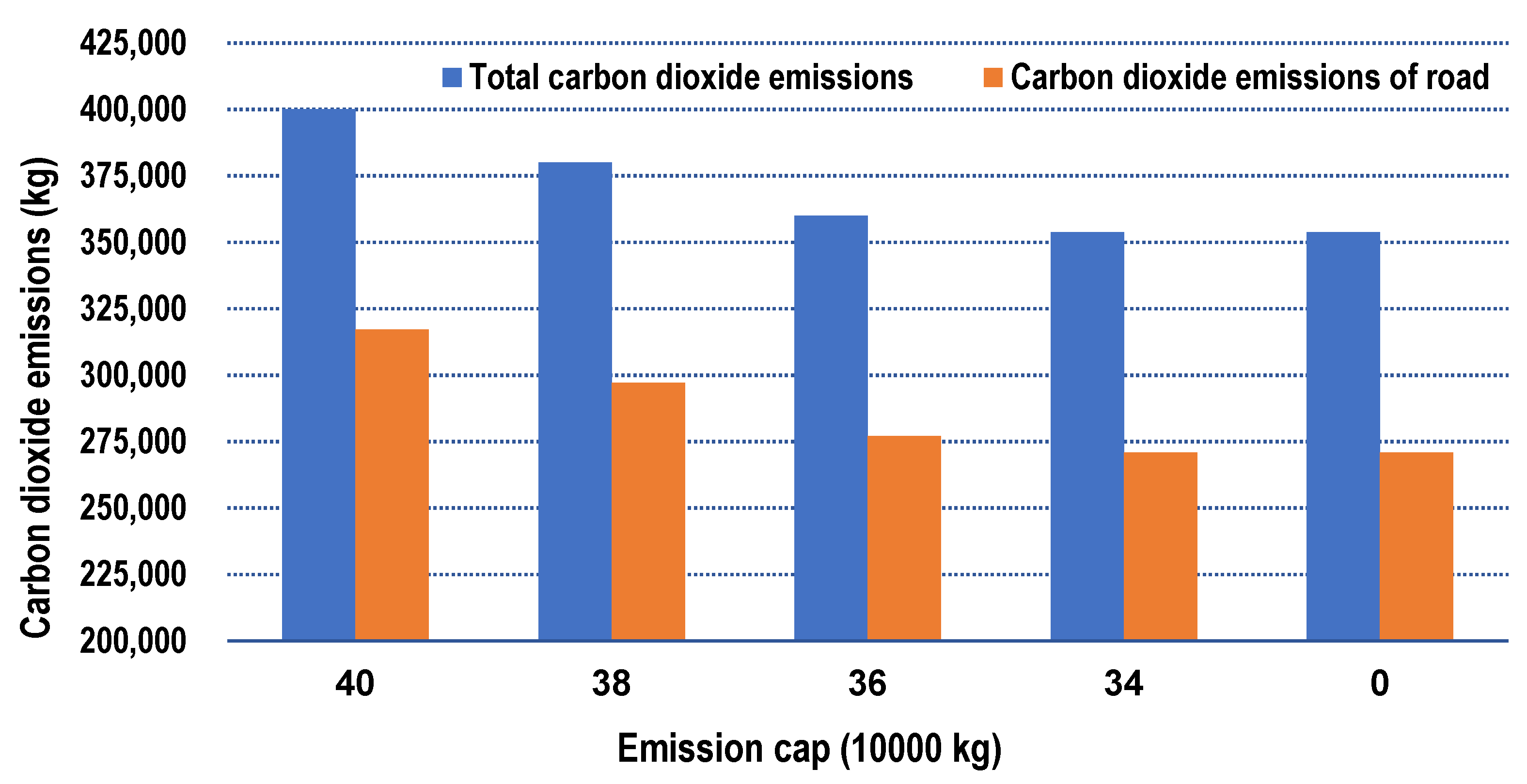
6.2.1. Analysis on the Effects of the Emission Cap on the Optimization Results

In this section, this study analyzed the optimization results given by the RPP model under different emission caps to reveal the effect of the emission cap on the optimization and compare the performances of the carbon cap-and-trade and tax policies. The emission cap was varied from 400,000 to 300,000 kg with a step of 20,000 kg, while other interactive parameters of the RPP model remained unchanged as listed in

Table 4. Optimization results under different emission caps.

Emission Cap (kg)	Carbon Cap-and-Trade Policy						Carbon Tax Policy
	400,000	380,000	360,000	340,000	320,000	300,000	0
Total Costs (CNY)	2,469,345	2,467,950	2,466,949	2,467,495	2,468,295	2,469,095	2,481,095
Expected Costs (CNY)	2,466,960	2,465,565	2,464,564	2,464,973	2,465,573	2,466,173	2,475,173
Optimality Robustness Costs (CNY)	0.15	0.10	0.08	137	337	537	3538
Feasibility Robustness Costs (CNY)	2385	2385	2385	2385	2385	2385	2385
Carbon Dioxide Emissions (kg)	400,015	380,009	360,008	353,657	353,657	353,657	353,657

. Meanwhile, the emission cap was also set to 0, which makes the proposed routing problem regulated under the carbon tax policy. The optimization results under different emission caps are given in Table 4.

Table 4 demonstrates that increasing the emission cap did not improve but worsen the reduction of carbon dioxide emissions. Although the carbon cap-and-trade policy reduced the total costs and considerably improved the optimality robustness of the optimization results of the RPP model, the comparison between them on reducing carbon dioxide emissions showed that the cap-and-trade policy did not always perform better than the carbon tax policy, because the carbon tax policy charges for all the carbon dioxide emissions, while the carbon cap-and-trade policy only covered the emissions that exceed the emission cap, which has also been claimed by Chen et al. [38]. The determination of the emission cap should be taken seriously when using the carbon cap-and-trade policy. In Table 4, the emission cap of 320,000 kg is suitable when the intermodal operator attaches great importance to environmental sustainability, since this emission cap leads to the same emissions to the carbon tax policy, while reduces the total costs. In this case, the carbon cap-and-trade policy was more motivating than the carbon tax policy by providing a higher cost-effective routing solution, which can also enhance the willingness of decision makers to implement the policy. Table 4 also finds that the feasibility robustness was not influenced by the carbon reduction policies, since its formulation was only related to uncertain capacities.

Following the above analysis, this study found that the travel costs of routing and carbon dioxide emissions of road services have variations illustrated by Figure 4 when the emission cap changed. As shown in Figure 4, the travel costs of the distribution routes remained unchanged when the emission cap decreased to reduce the carbon dioxide emissions. This situation meant that the distribution route design decision did not change during the emission reduction process and further indicated that the selected transportation services are the same. Consequently, the distribution route design decision did not contribute to the carbon dioxide emission reduction in this case.

On contrary, Figure 4 shows that the carbon dioxide emissions of road were extensively reduced in this process. Checking Table 4 and Figure 4 identifies that the reduced volume of carbon dioxide emissions of road services was equal to the decrease of the total carbon dioxide emissions, illustrated by Figure 5. In the proposed routing problem, reducing carbon dioxide emissions mainly depended on the distribution route design and the truck speed optimization. When the distribution route design was kept unchanged, it is the truck speed optimization that worked to lower the carbon dioxide emissions. Therefore, this study concluded that it is necessary to integrate truck speed optimization into the routing to strengthen the environmental sustainability.

6.2.2. Analysis on the Effects of the Multiple Time Windows on the Optimization Results

Multiple time windows are also an important approach considered by this study to improve the performance of the proposed routing. To verify whether this consideration can lead to a comprehensive improvement, this section designed 4 cases where each transportation order was equipped with one pickup time window and one delivery time window that were randomly selected from their multiple settings before problem solving. Then, based on the setting of the interactive parameters in Table 2, this study obtained the solutions to the three cases without time window selection decision. Comparisons between the solutions to the routing with and without multiple time windows are shown in Figure 6. In this figure, Case No.1 considered multiple time windows for pickups and deliveries, while Cases No.2 to No.5 considered a single time window.

As illustrated by Figure 6, the RPP model with multiple time windows gave the solution to the road-rail intermodal routing problem that obtained the minimum values for the total costs, expected costs, optimality robustness costs and carbon dioxide emissions. However, the feasibility robustness costs were constant regardless of the setting of the time window(s), since this robustness was only associated with the uncertain capacities. The comparisons clearly clarify that the economic and environmental sustainability objectives of the road-rail intermodal routing considerably benefit from the use of multiple time windows. Meanwhile, the multiple time windows enhanced the optimality robustness, which lowered the objective function risks and improved the average performance of the routing optimization. Therefore, considering multiple time windows improved the comprehensive performance of the routing optimization.

Multiple time windows can enhance the customer flexibility and further improve the flexibility of the routing decision-making. Therefore, the intermodal operator can obtain higher flexibility when making tradeoffs between the time window selection and objective improvement. Moreover, multiple time windows made the optimization model of the routing problem yield a lager solution space that covered solutions whose comprehensive performances were better than the use of a single time window setting. Consequently, the routing optimization associated with multiple time windows can achieve the improvement on the economy, optimality robustness and environmental sustainability. Above all, considering multiple time windows in the routing optimization is a meaningful extension.

6.2.3. Analysis on the Effects of the Truck Operations Optimization on the Optimization Results

In this section, this study first excluded truck departure time planning from the road-rail intermodal routing by letting ${\lambda }_i^k=y_i^k$ for $\forall k\in K$ and $\forall i\in {\mathsf{\Gamma }}_{{\tau }_k^{+}}^{-}$. However, the RPP model failed to find a feasible solution to the problem due to the violation of the road traffic restrictions and time window constraints. Therefore, truck departure time planning was essential in the proposed routing and builds the foundation of the optimization. This section then focused on evaluating the effects of the truck speed optimization on the performances of the optimization results. This section designed four cases where the trucks of each road service were assigned to a speed to exclude truck speed optimization from the road-rail intermodal routing in order to compare the optimization results of the RPP model with and without truck speed optimization. Figure 7 shows the comparisons in which Case No.1 is associated with the truck speed optimization, while Cases No.2 to No.5 neglect such an optimization.

Figure 7 explains that the truck speed optimization enabled the RPP model for road-rail intermodal routing to obtain the best performances on lowering costs, improving optimality robustness and reducing carbon dioxide emissions, which showed similar effects to the multiple time windows. The contribution to emission reduction of the truck speed optimization was also verified in Section 6.2. As illustrated by Figure 7, the feasibility robustness of the RPP model remains constant. Therefore, neither multiple time windows nor truck speed optimization influenced the model’s feasibility robustness. Above all, besides multiple time windows, the comprehensive performance of the routing significantly benefited from the truck operations optimization.

In the proposed routing problem, the carbon dioxide emission reduction contributed by the truck speed optimization helped to decrease the difference between the total emissions of the routing plan and the emission cap, and further lower the optimality robustness costs under the carbon cap-and-trade policy where the trading price rate was uncertain. Besides reducing the emissions, the truck speed optimization also helped to lower the inventory costs by optimizing the arrival times of the containers at the transshipping nodes to cut down on their waiting periods. Therefore, the improvement on the economy, optimality robustness and environmental sustainability can be achieved by the truck speed optimization. As a result, it is necessary to integrate truck operations optimization into road-rail intermodal routing, in which the discrete speed option approach and speed-dependent emission modeling based on MEET show good feasibility.

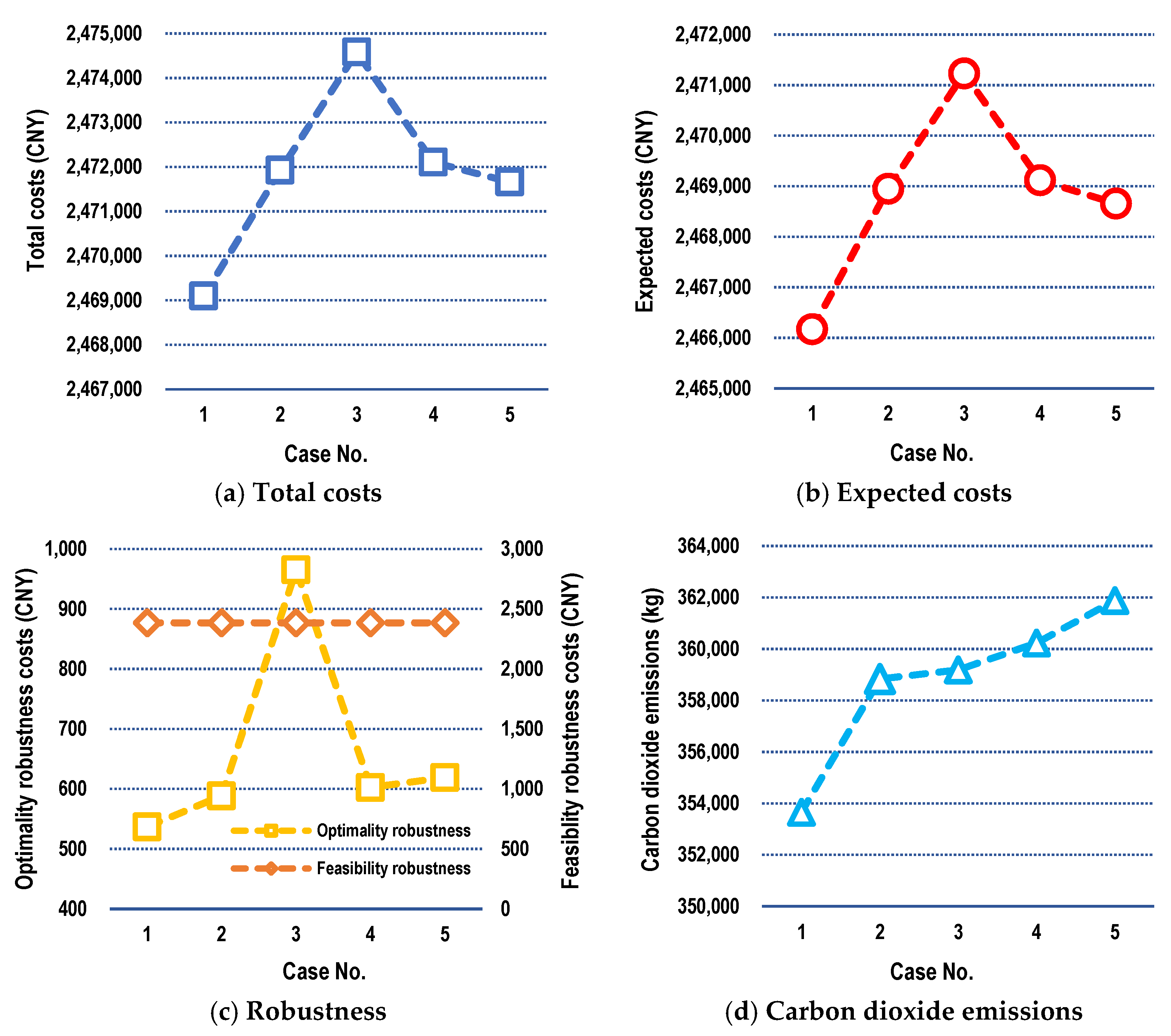
6.2.4. Sensitivity Analysis

In this section the author conducted a sensitivity analysis on the optimization results of the RPP model with respect to the interactive parameters related to the robustness, which provided a range of optimal solutions for various scenarios resulting from the dynamics of real-time decision making. Then, the most suitable solutions could be selected based on the decision makers’ preference. In this study, $\delta$ was the penalty costs for violating the uncertain capacity constraint. Its value can be only determined by using real-time information in a given scenario [64]. Therefore, $\delta$ was not considered in the sensitivity analysis. By varying $\gamma$ from 0.4 to 1.0 with a step of 0.2 and ${\alpha }_0$ from 0.5 to 1.0 with a step of 0.1, while keeping $\delta$ = 30 and $cap$= 300,000, efficient solutions were obtained by using the RPP model. The optimization results are given in

Table 5. Sensitivity of the RPP solutions to the proposed routing with respect to $\gamma$ and ${\alpha }_0$.

$\mathit{\gamma }$	${\mathit{\alpha }}_0$	Expected Costs (CNY)	Optimality Robustness Costs (CNY)	Feasibility Robustness Costs (CNY)	Total Costs (CNY)	Carbon Dioxide Emissions (kg)
0.4	0.5	2,466,173	429	2385	2,468,988	353,657
	0.6	2,471,574	423	1908	2,473,905	352,861
	0.7	2,477,946	401	0	2,478,347	350,065
	0.8	2,477,946	401	0	2,478,347	350,065
	0.9	2,477,946	401	0	2,478,347	350,065
	1.0	2,477,946	401	0	2,478,347	350,065
0.6	0.5	2,466,173	644	2385	2,469,202	353,657
	0.6	2,471,574	634	1908	2,474,117	352,861
	0.7	2,477,946	601	0	2,478,547	350,065
	0.8	2,477,946	601	0	2,478,547	350,065
	0.9	2,477,946	601	0	2,478,547	350,065
	1.0	2,477,946	601	0	2,478,547	350,065
0.8	0.5	2,466,173	859	2385	2,469,417	353,657
	0.6	2,471,574	846	1908	2,474,328	352,861
	0.7	2,477,946	801	0	2,478,747	350,065
	0.8	2,477,946	801	0	2,478,747	350,065
	0.9	2,477,946	801	0	2,478,747	350,065
	1.0	2,477,946	801	0	2,478,747	350,065
1.0	0.5	2,466,173	1073	2385	2,469,632	353,657
	0.6	2,471,574	1057	1908	2,474,539	352,861
	0.7	2,477,946	1001	0	2,478,948	350,065
	0.8	2,477,946	1001	0	2,478,948	350,065
	0.9	2,477,946	1001	0	2,478,948	350,065
	1.0	2,477,946	1001	0	2,478,948	350,065

.

In the sensitivity analysis shown in Table 5, it was found that the optimization results of the RPP model were sensitive to ${\alpha }_0$, when ${\alpha }_0$ varies from 0.5 to 0.7. The sensitivity showed that the total costs of the proposed routing increased with the increase of ${\alpha }_0$. It is indicated that the feasibility robustness costs became insensitive when ${\alpha }_0$ exceeds 0.7 and are reduced to 0 under this situation, which means that the capacity constraint was entirely satisfied at all times. Based on the changes of the optimization results when ${\alpha }_0$ varies, it was concluded that improving the confidence level enhances the robustness, reduces the carbon dioxide emissions, while increasing the expected costs of the solutions. The increase of the expected costs was more significant than the decrease of the robustness costs, and thereby led to an increase in the total costs. Therefore, reducing the total costs conflicted with the improvement of robustness and environmental sustainability in the proposed routing, requiring the intermodal operator to make tradeoffs based on customers’ preferences. However, the expected costs, feasibility robust costs and carbon dioxide emissions of the optimization results were insensitive to $\gamma$, and increasing $\gamma$ only led to the increase in the optimality robustness costs and the total costs.

6.3. Findings

Implementing and evaluating the proposed model and solution approach in an empirical case found the following insights that can help an intermodal operator to organize an efficient road-rail intermodal transportation and provide customers with the best transportation services:

(1)

The RPP model was more efficient than the BPCCP model in optimizing the routing problem by providing higher cost-efficient solutions and enhancing the robustness of the solutions.

(2)

The carbon cap-and-trade policy reduced the total costs and optimized the optimality robustness of the routing problem when compared with the carbon tax policy.

(3)

When reducing carbon dioxide emissions was the primary goal, the carbon cap-and-trade policy did not always work better than the carbon tax policy. However, when the two policies achieved the same performance on emission reduction, the carbon cap-and-trade policy was more suitable and motivating to be adopted due to its advantages in improving both the economy and robustness of the routing.

(4)

The carbon cap-and-trade policy in a fuzzy environment depended on the design of a suitable emission cap to improve its performance and should be attached with great importance by intermodal operators.

(5)

Multiple time windows and truck operations optimization significantly strengthened the comprehensive performance of the routing by reducing the costs, improving the optimality robustness, and lowering the carbon dioxide emissions.

(6)

In the truck operations optimization, the truck departure time planning ensured that a feasible routing decision can be made under road traffic restrictions.

(7)

Improving the confidence level provided a solution to enhance the robustness and reduce the carbon dioxide emissions of the routing. However, it caused an increase in the total costs. The intermodal operator thus needs to make tradeoffs in this conflicting situation.

7. Conclusions

This study investigated a road-rail intermodal routing problem making the following contributions to improve the problem optimization:

(1)

A green road-rail intermodal routing that models both schedule-based and flexible services in a road-rail intermodal hub-and-spoke network and considers capacity uncertainty was explored to make the problem match the realistic transportation scenario.

(2)

The carbon cap-and-trade policy was introduced into the routing, in which the uncertainty of the carbon trading price was formulated. The performance of the carbon cap-and-trade policy was systematically discussed by comparison with the carbon tax policy.

(3)

Multiple time windows and truck operations optimization under road traffic restrictions were integrated into the routing to make the problem more realistic and was verified to be able to improve the comprehensive performance of the problem optimization.

(4)

A robust possibilistic programming approach was developed to deal with the problem and showed good feasibility on obtaining efficient solutions to the dynamic and uncertain decision-making environment.

Based on the empirical case study, several insights that can help the intermodal operator to organize an efficient transportation and provide customers with the best services are then summarized in Section 6.3.

However, this study only considers limited sources of uncertainty in the road-rail intermodal transportation system. Uncertainty of time and demand is not formulated in this study. Moreover, this study depends on the exact solution algorithm to obtain the solutions to the problem. The road-rail intermodal routing problem is NP hard. This solution approach may be infeasible when the problem becomes more complex by considering more sources of uncertainty or the scale of the case becomes larger due to the increase of the transportation orders and expansion of the transportation network.

Consequently, multiple sources of uncertainty in the transportation system will be discussed by the future research. The feasibility of the exact solution algorithm will be tested to check if it can efficiently solve the road-rail intermodal routing problem with multiple sources of uncertainty in a large-scale case. Heuristic algorithms will be designed for such a problem and their computational accuracy and efficiency will be further verified by comparison with the exact solution algorithm. Additionally, it is worthy to use other forms of robust optimization (e.g., robust possibilistic flexible programming [82]) and improved definitions of fuzzy numbers (e.g., Type-II fuzzy numbers [83]) that can better model the uncertainty to address the routing problem proposed by this study.

References

1. Hosseini, S.; Al Khaled, A. Freight flow optimization to evaluate the criticality of intermodal surface transportation system infrastructures. Comput. Ind. Eng. 2021, 159, 107522. [Google Scholar] [CrossRef]
2. Delbart, T.; Molenbruch, Y.; Braekers, K.; Caris, A. Uncertainty in intermodal and synchromodal transport: Review and future research directions. Sustainability 2021, 13, 3980. [Google Scholar] [CrossRef]
3. Zhang, H.; Li, Y.; Zhang, Q.; Chen, D. Route selection of multimodal transport based on China railway transportation. J. Adv. Transp. 2021, 2021, 9984659. [Google Scholar] [CrossRef]
4. Guo, W.; Atasoy, B.; Negenborn, R.R. Global synchromodal shipment matching problem with dynamic and stochastic travel times: A reinforcement learning approach. Ann. Oper. Res. 2022, 1–32. [Google Scholar] [CrossRef]
5. Bierwirth, C.; Kirschstein, T.; Meisel, F. On transport service selection in intermodal rail/road distribution networks. Bus. Res. 2012, 5, 198–219. [Google Scholar] [CrossRef]
6. Heggen, H.; Molenbruch, Y.; Caris, A.; Braekers, K. Intermodal container routing: Integrating long-haul routing and local drayage decisions. Sustainability 2019, 11, 1634. [Google Scholar] [CrossRef]
7. Wang, Q.Z.; Chen, J.M.; Tseng, M.L.; Luan, H.M.; Ali, M.H. Modelling green multimodal transport route performance with witness simulation software. J. Clean. Prod. 2020, 248, 119245. [Google Scholar] [CrossRef]
8. Caris, A.; Macharis, C.; Janssens, G.K. Decision support in intermodal transport: A new research agenda. Comput. Ind. 2013, 64, 105–112. [Google Scholar] [CrossRef]
9. Sun, Y.; Yu, N.; Huang, B. Green road–rail intermodal routing problem with improved pickup and delivery services integrating truck departure time planning under uncertainty: An interactive fuzzy programming approach. Complex Intell. Syst. 2022, 8, 1459–1486. [Google Scholar] [CrossRef]
10. Flodén, J.; Bärthel, F.; Sorkina, E. Transport buyers choice of transport service–A literature review of empirical results. Res. Transp. Bus. Manag. 2017, 100, 35–45. [Google Scholar] [CrossRef]
11. Barnhart, C.; Ratliff, H.D. Modeling intermodal routing. J. Bus. Logist. 1993, 14, 205. [Google Scholar]
12. Macharis, C.; Bontekoning, Y.M. Opportunities for OR in intermodal freight transport research: A review. Eur. J. Oper. Res. 2004, 153, 400–416. [Google Scholar] [CrossRef]
13. Zweers, B.G.; van der Mei, R.D. Minimum costs paths in intermodal transportation networks with stochastic travel times and overbookings. Eur. J. Oper. Res. 2022, 300, 178–188. [Google Scholar] [CrossRef]
14. Ahmady, M.; Eftekhari Yeghaneh, Y. Optimizing the cargo flows in multi-modal freight transportation network under disruptions. Iran. J. Sci. Technol. Trans. Civ. Eng. 2022, 46, 453–472. [Google Scholar] [CrossRef]
15. Epicoco, N.; Falagario, M. Decision support tools for developing sustainable transportation systems in the EU: A review of research needs, barriers, and trends. Res. Transp. Bus. Manag. 2022, 43, 100819. [Google Scholar] [CrossRef]
16. Zhang, Y.; Guo, W.; Negenborn, R.R.; Atasoy, B. Synchromodal transport planning with flexible services: Mathematical model and heuristic algorithm. Transp. Res. Part C Emerg. Technol. 2022, 140, 103711. [Google Scholar] [CrossRef]
17. Wang, S.; Zhang, Q.; Wang, W. The impact of carbon abatement policies on port intermodal freight transportation routing and cost. In Proceedings of the International Conference on Electrical and Information Technologies for Rail Transportation, Changsha, China, 20–22 October 2017; Springer: Singapore; pp. 689–699. [Google Scholar]
18. He, P.; Zhang, W.; Xu, X.; Bian, Y. Production lot-sizing and carbon emissions under cap-and-trade and carbon tax regulations. J. Clean. Prod. 2015, 103, 241–248. [Google Scholar] [CrossRef]
19. Dua, A.; Sinha, D. Quality of multimodal freight transportation: A systematic literature review. World Rev. Intermodal Transp. Res. 2019, 8, 167–194. [Google Scholar] [CrossRef]
20. Dragomir, A.G.; Doerner, K.F. Solution techniques for the inter-modal pickup and delivery problem in two regions. Comput. Oper. Res. 2020, 113, 104808. [Google Scholar] [CrossRef]
21. Schaap, H.; Schiffer, M.; Schneider, M.; Walther, G. A large neighborhood search for the vehicle routing problem with multiple time windows. Transp. Sci. 2022. [Google Scholar] [CrossRef]
22. Baltz, A.; El Ouali, M.; Jäger, G.; Sauerland, V.; Srivastav, A. Exact and heuristic algorithms for the travelling salesman problem with multiple time windows and hotel selection. J. Oper. Res. Soc. 2015, 66, 615–626. [Google Scholar] [CrossRef]
23. Wang, R.; Yang, K.; Yang, L.; Gao, Z. Modeling and optimization of a road–rail intermodal transport system under uncertain information. Eng. Appl. Artif. Intel. 2018, 72, 423–436. [Google Scholar] [CrossRef]
24. Hosseini, A.; Pishvaee, M.S. Capacity reliability under uncertainty in transportation networks: An optimization framework and stability assessment methodology. Fuzzy Optim. Decis. Mak. 2022, 21, 479–512. [Google Scholar] [CrossRef]
25. Sun, Y.; Zhang, G.; Hong, Z.; Dong, K. How uncertain information on service capacity influences the intermodal routing decision: A fuzzy programming perspective. Information 2018, 9, 24. [Google Scholar] [CrossRef]
26. Sun, Y. Fuzzy approaches and simulation-based reliability modeling to solve a Road–Rail intermodal routing problem with soft delivery time windows when demand and capacity are uncertain. Int. J. Fuzzy Syst. 2020, 22, 2119–2148. [Google Scholar] [CrossRef]
27. Haddadsisakht, A.; Ryan, S.M. Closed-loop supply chain network design with multiple transportation modes under stochastic demand and uncertain carbon tax. Int. J. Prod. Econ. 2018, 195, 118–131. [Google Scholar] [CrossRef]
28. Alizadeh, M.; Ma, J.; Marufuzzaman, M.; Yu, F. Sustainable olefin supply chain network design under seasonal feedstock supplies and uncertain carbon tax rate. J. Clean. Prod. 2019, 222, 280–299. [Google Scholar] [CrossRef]
29. Hu, H.; Li, X.; Zhang, Y.; Shang, C.; Zhang, S. Multi-objective location-routing model for hazardous material logistics with traffic restriction constraint in inter-city roads. Comput. Ind. Eng. 2019, 128, 861–876. [Google Scholar] [CrossRef]
30. Sung, I.; Nielsen, P. Speed optimization algorithm with routing to minimize fuel consumption under time-dependent travel conditions. Prod. Manuf. Res. 2020, 8, 1–19. [Google Scholar] [CrossRef]
31. Sun, Y.; Lang, M. Modeling the multicommodity multimodal routing problem with schedule-based services and carbon dioxide emission costs. Math. Probl. Eng. 2015, 2015, 406218. [Google Scholar] [CrossRef]
32. Duan, X.; Heragu, S. Carbon Emission Tax Policy in an Intermodal Transportation Network. In Proceedings of the IIE Annual Conference, Nashville, TN, USA, 30 May–2 June 2015; Institute of Industrial and Systems Engineers (IISE): Norcross, GA, USA; pp. 566–574. [Google Scholar]
33. Zhang, D.; He, R.; Li, S.; Wang, Z. A multimodal logistics service network design with time windows and environmental concerns. PLoS ONE 2017, 12, e0185001. [Google Scholar] [CrossRef] [PubMed] [Green Version]
34. Guo, W.; Atasoy, B.; Beelaerts van Blokland, W.; Negenborn, R.R. A global intermodal shipment matching problem under travel time uncertainty. In International Conference on Computational Logistics; Springer: Cham, Switzerland, 2020; pp. 553–568. [Google Scholar]
35. Hrušovský, M.; Demir, E.; Jammernegg, W.; Van Woensel, T. Hybrid simulation and optimization approach for green intermodal transportation problem with travel time uncertainty. Flex. Serv. Manuf. J. 2018, 30, 486–516. [Google Scholar] [CrossRef]
36. Maiyar, L.M.; Thakkar, J.J. Modelling and analysis of intermodal food grain transportation under hub disruption towards sustainability. Int. J. Prod. Econ. 2019, 217, 281–297. [Google Scholar] [CrossRef]
37. Qiu, Y.; Qiao, J.; Pardalos, P.M. A branch-and-price algorithm for production routing problems with carbon cap-and-trade. Omega 2017, 68, 49–61. [Google Scholar] [CrossRef]
38. Cheng, X.Q.; Jin, C.; Wang, C.; Mamatok, Y. Impacts of different low-carbon policies on route decisions in intermodal freight transportation: The case of the west river region in China. In Proceedings of the International Forum on Shipping, Ports and Airports (IFSPA), Hong Kong, China, 20–24 May 2019; pp. 281–293. [Google Scholar]
39. Xu, X.; Xu, X.; He, P. Joint production and pricing decisions for multiple products with cap-and-trade and carbon tax regulations. J. Clean. Prod. 2016, 112, 4093–4106. [Google Scholar] [CrossRef]
40. Bai, Q.; Chen, M. The distributionally robust newsvendor problem with dual sourcing under carbon tax and cap-and-trade regulations. Comput. Ind. Eng. 2016, 98, 260–274. [Google Scholar] [CrossRef]
41. Jharkharia, S.; Das, C. Vehicle routing analyses with integrated order picking and delivery problem under carbon cap and trade policy. Manag. Res. Rev. 2019, 43, 223–243. [Google Scholar] [CrossRef]
42. Ji, H.; Wu, P. Sailing route and speed optimization for green intermodal transportation. In Proceedings of the 2020 IEEE 5th International Conference on Intelligent Transportation Engineering (ICITE), Beijing, China, 11–13 September 2020; IEEE: Piscataway, NJ, USA; pp. 18–22. [Google Scholar]
43. Rosyida, E.E.; Santosa, B.; Pujawan, I.N. Freight route planning in intermodal transportation network to deal with combinational disruptions. Cogent Eng. 2020, 7, 1805156. [Google Scholar] [CrossRef]
44. Fazayeli, S.; Eydi, A.; Kamalabadi, I.N. Location-routing problem in multimodal transportation network with time windows and fuzzy demands: Presenting a two-part genetic algorithm. Comput. Ind. Eng. 2018, 119, 233–246. [Google Scholar] [CrossRef]
45. Sun, Y.; Li, X. Fuzzy programming approaches for modeling a customer-centred freight routing problem in the road-rail intermodal hub-and-spoke network with fuzzy soft time windows and multiple sources of time uncertainty. Mathematics 2019, 7, 739. [Google Scholar] [CrossRef]
46. Xie, L.; Cao, C. Multi-modal and multi-route transportation problem for hazardous materials under uncertainty. Eng. Optim. 2021, 53, 2180–2200. [Google Scholar] [CrossRef]
47. Maity, G.; Yu, V.F.; Roy, S.K. Optimum intervention in transportation networks using multimodal system under fuzzy stochastic environment. J. Adv. Transp. 2022, 2022, 3997396. [Google Scholar] [CrossRef]
48. Peng, Y.; Yong, P.; Luo, Y. The route problem of multimodal transportation with timetable under uncertainty: Multi-objective robust optimization model and heuristic approach. RAIRO-Oper. Res. 2021, 55, S3035–S3050. [Google Scholar] [CrossRef]
49. Fattahi, Z.; Behnamian, J. Hazardous materials transportation with focusing on intermodal transportation: A state-of-the-art review. Int. J. Ind. Eng. 2021, 28, 390–411. [Google Scholar]
50. Uddin, M.; Huynh, N. Reliable routing of road-rail intermodal freight under uncertainty. Netw. Spat. Econ. 2019, 19, 929–952. [Google Scholar] [CrossRef]
51. Sun, Y.; Hrušovský, M.; Zhang, C.; Lang, M. A time-dependent fuzzy programming approach for the green multimodal routing problem with rail service capacity uncertainty and road traffic congestion. Complexity 2018, 2018, 8645793. [Google Scholar] [CrossRef]
52. Lu, Y.; Lang, M.; Sun, Y.; Li, S. A fuzzy intercontinental road-rail multimodal routing model with time and train capacity uncertainty and fuzzy programming approaches. IEEE Access 2020, 8, 27532–27548. [Google Scholar] [CrossRef]
53. Sun, Y. Green and reliable freight routing problem in the road-rail intermodal transportation network with uncertain parameters: A fuzzy goal programming approach. J. Adv. Transp. 2020, 2020, 7570686. [Google Scholar] [CrossRef]
54. Pishvaee, M.S.; Razmi, J.; Torabi, S.A. Robust possibilistic programming for socially responsible supply chain network design: A new approach. Fuzzy Sets Syst. 2012, 206, 1–20. [Google Scholar] [CrossRef]
55. Sun, Y. A Fuzzy Multi-objective routing model for managing hazardous materials door-to-door transportation in the road-rail multimodal network with uncertain demand and improved service level. IEEE Access 2020, 8, 172808–172828. [Google Scholar] [CrossRef]
56. Hrušovský, M.; Demir, E.; Jammernegg, W.; Van Woensel, T. Real-time disruption management approach for intermodal freight transportation. J. Clean. Prod. 2021, 280, 124826. [Google Scholar] [CrossRef]
57. Wang, W.; Xu, X.; Jiang, Y.; Xu, Y.; Cao, Z.; Liu, S. Integrated scheduling of intermodal transportation with seaborne arrival uncertainty and carbon emission. Transp. Res. Part D Transp. Environ. 2020, 88, 102571. [Google Scholar] [CrossRef]
58. Shao, C.; Wang, H.; Yu, M. Multi-Objective Optimization of Customer-Centered Intermodal Freight Routing Problem Based on the Combination of DRSA and NSGA-III. Sustainability 2022, 14, 2985. [Google Scholar] [CrossRef]
59. Guo, W.; Atasoy, B.; van Blokland, W.B.; Negenborn, R.R. A dynamic shipment matching problem in hinterland synchromodal transportation. Decis. Support Syst. 2020, 134, 113289. [Google Scholar] [CrossRef]
60. Resat, H.G.; Turkay, M. A discrete-continuous optimization approach for the design and operation of synchromodal transportation networks. Comput. Ind. Eng. 2019, 130, 512–525. [Google Scholar] [CrossRef]
61. Yu, V.F.; Redi AA, N.; Jewpanya, P.; Lathifah, A.; Maghfiroh, M.F.; Masruroh, N.A. A simulated annealing heuristic for the heterogeneous fleet pollution routing problem. In Environmental Sustainability in Asian Logistics and Supply Chains; Springer: Singapore, 2018; pp. 171–204. [Google Scholar]
62. Demir, E.; Bektaş, T.; Laporte, G. The bi-objective pollution-routing problem. Eur. J. Oper. Res. 2014, 232, 464–478. [Google Scholar] [CrossRef]
63. Franceschetti, A.; Honhon, D.; Van Woensel, T.; Bektaş, T.; Laporte, G. The time-dependent pollution-routing problem. Transp. Res. Part B Methodol. 2013, 56, 265–293. [Google Scholar] [CrossRef]
64. Sun, Y.; Liang, X.; Li, X.; Zhang, C. A fuzzy programming method for modeling demand uncertainty in the capacitated road–rail multimodal routing problem with time windows. Symmetry 2019, 11, 91. [Google Scholar] [CrossRef]
65. Zhang, Y.; Li, X.; van Hassel, E.; Negenborn, R.R.; Atasoy, B. Synchromodal transport planning considering heterogeneous and vague preferences of shippers. Transp. Res. Part E Logist. Transp. Rev. 2022, 164, 102827. [Google Scholar] [CrossRef]
66. Xiao, Y.; Konak, A. The heterogeneous green vehicle routing and scheduling problem with time-varying traffic congestion. Transp. Res. Part E Logist. Transp. Rev. 2016, 88, 146–166. [Google Scholar] [CrossRef]
67. Hickman, J.; Hassel, D.; Joumard, R.; Samaras, Z.; Sorenson, S. Methodology for Calculating Transport Emissions and Energy Consumption. 1999. Available online: https://trimis.ec.europa.eu/sites/default/files/project/documents/meet.pdf (accessed on 7 July 2022).
68. Mahlke, D.; Martin, A.; Moritz, S. A mixed integer approach for time-dependent gas network optimization. Optim. Methods Softw. 2010, 25, 625–644. [Google Scholar] [CrossRef]
69. Xie, Y.; Lu, W.; Wang, W.; Quadrifoglio, L. A multimodal location and routing model for hazardous materials transportation. J. Hazard. Mater. 2012, 227, 135–141. [Google Scholar] [CrossRef] [PubMed]
70. Zahiri, B.; Tavakkoli-Moghaddam, R.; Pishvaee, M.S. A robust possibilistic programming approach to multi-period location–allocation of organ transplant centers under uncertainty. Comput. Ind. Eng. 2014, 74, 139–148. [Google Scholar] [CrossRef]
71. Habib, M.S.; Asghar, O.; Hussain, A.; Imran, M.; Mughal, M.P.; Sarkar, B. A robust possibilistic programming approach toward animal fat-based biodiesel supply chain network design under uncertain environment. J. Clean. Prod. 2021, 278, 122403. [Google Scholar] [CrossRef]
72. Salimian, S.; Mousavi, S.M. A robust possibilistic optimization model for organ transplantation network design considering climate change and organ quality. J. Ambient. Intell. Humaniz. Comput. 2022, 1–24. [Google Scholar] [CrossRef]
73. Kundu, P.; Kar, S.; Maiti, M. Multi-objective multi-item solid transportation problem in fuzzy environment. Appl. Math. Model. 2013, 37, 2028–2038. [Google Scholar] [CrossRef]
74. Zahiri, B.; Pishvaee, M.S. Blood supply chain network design considering blood group compatibility under uncertainty. Int. J. Prod. Res. 2017, 55, 2013–2033. [Google Scholar] [CrossRef]
75. Günay, E.E.; Kremer GE, O.; Zarindast, A. A multi-objective robust possibilistic programming approach to sustainable public transportation network design. Fuzzy Sets Syst. 2021, 422, 106–129. [Google Scholar] [CrossRef]
76. Chiadamrong DH, T.N.; Doan, T.H. A robust possibilistic chance-constrained programming model for optimizing a multi-objective aggregate production planning problem under uncertainty. J. Ind. Eng. Int. 2022; in press. [Google Scholar]
77. Delfani, F.; Kazemi, A.; SeyedHosseini, S.M.; Niaki, S.T.A. A novel robust possibilistic programming approach for the hazardous waste location-routing problem considering the risks of transportation and population. Int. J. Syst. Sci. Oper. Logist. 2021, 8, 383–395. [Google Scholar] [CrossRef]
78. Beheshtinia, M.A.; Salmabadi, N.; Rahimi, S. A robust possibilistic programming model for production-routing problem in a three-echelon supply chain. J. Model. Manag. 2021, 16, 1328–1357. [Google Scholar] [CrossRef]
79. Rabbani, M.; Hosseini-Mokhallesun, S.A.A.; Ordibazar, A.H.; Farrokhi-Asl, H. A hybrid robust possibilistic approach for a sustainable supply chain location-allocation network design. Int. J. Syst. Sci. Oper. Logist. 2020, 7, 60–75. [Google Scholar] [CrossRef]
80. Resat, H.G.; Turkay, M. Design and operation of intermodal transportation network in the Marmara region of Turkey. Transp. Res. Part E Logist. Transp. Rev. 2015, 83, 16–33. [Google Scholar] [CrossRef]
81. Zhang, X.; Yuan, X.; Jiang, Y. Optimization of multimodal transportation under uncertain demand and stochastic carbon trading price. Syst. Eng.—Theory Pract. 2021, 41, 2609–2620. [Google Scholar]
82. Habib, M.S.; Omair, M.; Ramzan, M.B.; Chaudhary, T.N.; Farooq, M.; Sarkar, B. A robust possibilistic flexible programming approach toward a resilient and cost-efficient biodiesel supply chain network. J. Clean. Prod. 2022, 366, 132752. [Google Scholar] [CrossRef]
83. J-Sharahi, S.; Khalili-Damghani, K.; Abtahi, A.R.; Rashidi-Komijan, A. Type-II fuzzy multi-product, multi-level, multi-period location–allocation, production–distribution problem in supply chains: Modelling and optimisation approach. Fuzzy Inf. Eng. 2018, 10, 260–283. [Google Scholar] [CrossRef] [Green Version]
Figure 1. Decision makings in the road-rail intermodal routing.
Systems 10 00156 g001
Figure 2. A trapezoidal fuzzy parameter.
Systems 10 00156 g002
Figure 3. Road-rail intermodal hub-and-spoke network in the case study.
Systems 10 00156 g003
Figure 4. Carbon dioxide emissions of road and travel costs of the distribution routes under different emission caps.
Systems 10 00156 g004
Figure 5. Variations of carbon dioxide emissions with respect to the emission cap.
Systems 10 00156 g005
Figure 6. Optimization results of the RPP model for the road-rail intermodal routing with and without multiple time windows.
Systems 10 00156 g006
Figure 7. Optimization results of the RPP model for the road-rail intermodal routing with and without truck speed optimization.
Systems 10 00156 g007