A Gaussian-Shaped Fuzzy Inference System for Multi-Source Fuzzy Data

Abstract

Fuzzy control theory has been extensively used in the construction of complex fuzzy inference systems. However, we argue that existing fuzzy control technologies focus mainly on the single-source fuzzy information system, disregarding the complementary nature of multi-source data. In this paper, we develop a novel Gaussian-shaped Fuzzy Inference System (GFIS) driven by multi-source fuzzy data. To this end, we first propose an interval-value normalization method to address the heterogeneity of multi-source fuzzy data. The contribution of our interval-value normalization method involves mapping heterogeneous fuzzy data to a unified distribution space by adjusting the mean and variance of data from each information source. As a result of combining the normalized descriptions from various sources for an object, we can obtain a fused representation of that object. We then derive an adaptive Gaussian-shaped membership function based on the addition law of the Gaussian distribution. GFIS uses it to dynamically granulate fusion inputs and to design inference rules. This proposed membership function has the advantage of being able to adapt to changing information sources. Finally, we integrate the normalization method and adaptive membership function to the Takagi–Sugeno (T–S) model and present a modified fuzzy inference framework. Applying our methodology to four datasets, we confirm that the data do lend support to the theory implying the improved performance and effectiveness.

1. Introduction

Traditional fuzzy control models have achieved remarkable success in making inferences for single-source fuzzy information systems. They have been increasingly applied to intelligent driving [1,2,3], intelligent medical [4,5,6], intelligent factories [7,8,9], and various other fields. It is believed that information fusion enhances the descriptive ability of objects through the use of data redundancy and complementarity [10,11,12]. A Fuzzy Inference System (FIS) could be improved by combining information fusion theory with fuzzy control theory to enable the system to perform better in terms of control and decision-making tasks than before. Motivated by this, we examine a fuzzy inference model that is driven by multi-source fuzzy data and look at how multi-source fuzzy data affect the precision of the inference model.

The fuzzy set (FS) and the rough set (RS) are two commonly used methods for describing fuzzy data or knowledge in a different way. As far back as 1965, scholar Zade was the first to propose the fuzzy set theory [13]. Its essence is to mine the decision-making value of fuzzy data by constructing membership functions and performing fuzzy set operations. Zadeh’s fuzzy set is modeled as:

$$A=A\left(x_1\right)/x_1+A\left(x_2\right)/x_2+\cdots +A\left(x_n\right)/x_n,$$

(1)

where $A\left(x_i\right)$ represents the membership degree of $x_1$ in set A, and “+” represents the component connection symbol in a fuzzy set; see [13]. Rough set theory was first proposed by Pawlak in 1982 [14]. The core idea is to use equivalence relation R to construct the equivalence class of object x in universe U. The approximation set composed of equivalent objects is called the lower approximation set, denoted as:

$$\underline{R\left(x\right)}=\{x\in U|{\left[x\right]}_R\subseteq U\},$$

(2)

see [15]. In contrast, the approximation set composed of equivalent objects and similar objects is called the upper approximation set, denoted as:

$$\overline{R\left(x\right)}=\{x\in U|{\left[x\right]}_R\cap U\ne \varnothing \},$$

(3)

see [15]. A key aspect of using fuzzy set theory to describe fuzzy knowledge lies in modeling membership functions [16]. There are four candidates for membership functions: bell-shaped curve function [17], S-shaped curve function [18], Z-shaped curve function [19], and $\pi$-shaped curve function [20]. Theoretically, the bell-shaped curve function is most widely used because it follows the law of large numbers and the central limit theorem [21,22].

Unfortunately, bell-shaped curve functions do not directly work for fuzzy systems involving multiple sources, for two reasons. First, it requires the function input to be a continuous and accurate real number. Second, it requires data from different sources to be analyzed using the same metrics so that comparability of data can be ensured. Our solution to these two problems is to use interval values to represent fuzzy data (such as measurement errors, degrees, spatial and temporal distances, emotions, etc.) and then to normalize heterogeneous fuzzy data to exact real numbers using interval normalization. Upon normalization, these real numbers will all be subjected to the same quantization factor (mean and variance). Additionally, we propose an adaptive membership function model that considers the dynamics of a multi-source environment, such as different information sources joining and leaving the system. With the aid of the membership function model, not only are we able to represent the overall distribution of data from multiple sources, but we are also able to adjust the membership value of the input variables to accommodate dynamic changes in the data. Combining the normalization method with the adaptive membership function, we develop a Gaussian-shaped Fuzzy Inference System (GFIS) driven by multi-source fuzzy data.

Our article makes two contributions to this literature. The first contribution is to propose an interval normalization method that is based on the normalization idea of Z-scores [23], and describe the meaning of fuzzy data by the standard deviations of each data value from the mean. The interval normalization method can be formalized as:

$$N_x=\frac{0.5\times \left(\underline{x}+\overline{x}\right)-\mu }{\sigma },$$

(4)

where $x=\left[\underline{x},\overline{x}\right]$ is an interval. The greatest challenge and innovation of our method lies in calculating mean $\mu$ and variance $\sigma$ for fuzzy data. In this work, we present formal models for mean and variance of fuzzy data, and we develop an approach for normalizing fuzzy data (interval value) with these formal models. The interval-value representation and normalization of fuzzy data are the premise of designing the fuzzy model of input variables in GFIS.

The second contribution of this article consists of deriving a Gaussian-shaped membership function for the input variable in GFIS. This function can be used to analyze normal-distributed data, and we denote it as:

$$\mathsf{\mu }\left(x\right)=f\left(N\right(x|0,m)),$$

(5)

where m is the number of information sources. A significant advantage of the proposed membership function lies in its ability to be adapted to the change of information sources. As a general rule, membership functions based on Gaussian distributions require dynamic mean and variance parameters to be specified as hyperparameters. When function variables are normalized in advance, we can ensure that the mean value of function variables is always 0 and that variance increases linearly with the number of information sources available. Therefore, we do not have to incur large computational costs to obtain the hyperparameters of Gaussian-shaped membership functions. Additionally, a Gaussian-shaped membership function can handle dynamic changes in information sources effectively. It is important to note that the GFIS, which comprises the normalization method and Gaussian-shaped membership function, is thus applicable to multi-source fuzzy environments.

The rest of the article is organized as follows: Section 2 provides a selected literature overview. Section 3 introduces preliminaries. Section 4 outlines the methodology proposed. Section 5 details the experimental design and Section 6 reports the experimental results. In Section 7, we present the conclusions.

2. Related Work

Due to its smoothness and ability to reflect people’s thinking characteristics, the Gaussian membership function has been widely used. Below, we provide a brief description of several Gaussian membership function methods and their applications in the literature. It is worth mentioning that our method (among the three alternatives discussed) is the only one that takes into account both data heterogeneity and fuzzy data fusion.

Hosseini et al. presented a Gaussian interval type-2 membership function and applied it to the classification of lung CAD (Computer Aided Design) [24]. Type-2 interval membership functions extend type-1 interval membership functions. In the type-2 fuzzy system, the membership of the type-1 fuzzy set is also characterized by a fuzzy set, which can improve the ability to deal with uncertainties. However, there are additional theoretical and computational challenges associated with the Gaussian interval type-2 membership function.

In Kong et al.’s study, a Gaussian membership function combined with a neural network model was designed to help diagnose automobile faults [25]. The system has been proven to perform better in terms of reasoning accuracy than either a network model or a fuzzy inference model alone. However, it relies on a single source of information to derive fuzzy inferences from multivariable data.

Li et al. proposed a Gaussian fuzzy inference model for multi-source homogeneous data [26]. The model uses three indicators (center representation, population, and density function) to describe single-source information and adopts a mixed Gaussian model to represent multi-source fusion information. This model does not address the heterogeneity and fuzziness of multi-source data. In addition, the model fails to account for differences between variables in a multidimensional dataset in terms of magnitude and measurement standards.

In previous research, different fuzzy inference models and membership functions were proposed for various practical applications. We propose a Gaussian fuzzy control inference model to solve the fuzzy inference problem in a multi-source fuzzy environment. Our model can improve medical CAD diagnostic accuracy by fusing X-ray images from different institutions. For automobile fault diagnosis, our model can describe each diagnosis parameter with fuzzy data. By further modeling these fuzzy parameters with fuzzy sets, we enhance fuzzy systems’ ability to cope with uncertainty. The fuzzy normalization model for multi-source data fusion enables us to map multivariate data to a dimensionless distribution space to ensure that the data metrics are aligned.

3. Preliminary

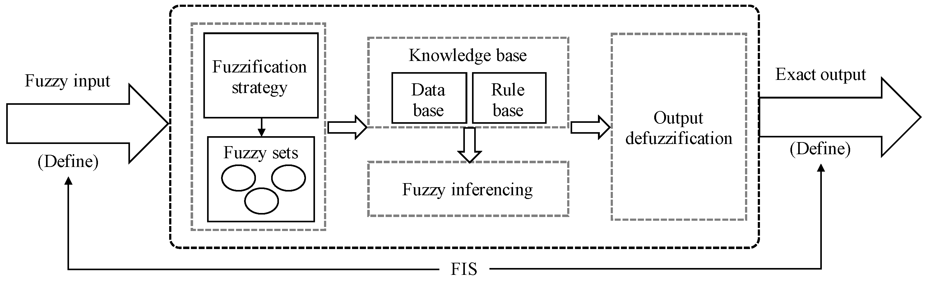
The Fuzzy Inference System (FIS), also known as a fuzzy system, is a software application that utilizes fuzzy set theory and fuzzy inference technology to process fuzzy information. In order to illustrate FIS’s application scenarios, let us take car following as an example. Due to the fact that the driver’s behavior is fuzzy and uncertain during the process of controlling the car, it can be difficult to accurately describe the driver’s behavior. When a car follows another car, it is necessary to maintain a safe distance in order to ensure the safety of drivers. FIS can be used to control the distance between a car and the one it is following. Specifically, based on the driver’s experience, the fuzzy rules of FIS for car following are summarized as follows. When a driver believes that the relative distance is far greater than the safe distance and the relative speed is fast, he or she accelerates appropriately. This will make the difference between the relative and safe distances as small as possible.

The classical FIS consists of five basic components: the definition of inputs and outputs; the construction of fuzzification strategies; the construction of knowledge bases; the design of fuzzy inference mechanisms; and the defuzzification of output. See Figure 1 for details.

(1) The definition of inputs and outputs

In an FIS, the inputs and outputs correspond to the observation variables and operation variables, respectively. Definition of inputs and outputs includes determining parameters, variable numbers, data formats, etc. An FIS that has one input variable is called a single variable FIS and an FIS that has more than one input variable is called a multivariable FIS. FIS driven by multi-source fuzzy data encounters challenges in normalizing heterogeneous fuzzy data due to the fact that the traditional method of normalizing data fails in this situation.

(2) The construction of fuzzification strategies

Fuzzification is the process of assigning each input variable to a fuzzy set with a certain degree of membership. An input variable can be either an exact value or fuzzy data with noise [27]. It is therefore necessary to consider the format of input variables when developing a strategy for fuzzification. In particular, fuzzy data are typically presented in discrete nominal formats or in aggregate interval-value formats, which makes mathematical fitting of membership functions challenging. In this paper, we use interval normalization to convert heterogeneous fuzzy data into continuous and exact values. We also use a math function to derive the membership function for fuzzy data.

(3) The construction of knowledge bases

In a knowledge base, there are two parts: a database and a rule base, respectively [28]. Among the features in the database are membership functions, scale transformation factors, and fuzzy set variables. The rule base contains some fuzzy control conditions and fuzzy logic relationships.

(4) The design of fuzzy inference mechanisms

Fuzzy inference uses fuzzy control conditions and fuzzy logics to predict the future status of operating variables. This is the core of an FIS. In an FIS, syllogisms [29,30,31] are commonly used to make inferences, which can be expressed as follows:

Truth: IF $x_1$ is $A_1$, ⋯, and $x_n$ is $A_n$, THEN y is B.

Condition: $x_1$ is $A_1^{{}^{\prime }}$, ⋯, and $x_n$ is $A_n^{{}^{\prime }}$.

The inference result: y is $B^{{}^{\prime }}$.

According to the FIS, truth is represented by fuzzy implication relations, denoted as $A^{\underrightarrow{f\left(x\right)}}B$. The inference result is derived from the combination of fuzzy conditions and fuzzy logics.

(5) The defuzzification of output

In general, the result derived from the FIS is a fuzzy value or a set, which must be deblurred to identify a clear control signal or a decision output. Most commonly used defuzzification methods include the maximum membership [32], the weighted average [33], and the center of gravity [34].

Maximum Membership Given k FIS submodels, the output of each FIS submodel is $y_i$ with the membership degree of $\mu \left(x_i\right)$. The final output of the FIS model is given by:

$$y=y_i,$$

(6)

where

$$i=arg\underset{i}{max}\left\{\mu \left(x_1\right),\mu \left(x_2\right),\dots ,\mu \left(x_k\right)\right\},$$

(7)

see [32].

Weighted Average Given k FIS submodels, the output of each FIS submodel is $y_i$ with the membership degree of $\mu \left(x_i\right)$. The final output of the FIS model is:

$$y=\frac{{\sum }_{i=1}^{i=k}{y}_i\times \mu \left(x_i\right)}{k},$$

(8)

as k is the number of sub FIS models, see [33].

Center of Gravity Given k FIS submodels, the output of each FIS submodel is $y_i$ with the membership degree of $\mu \left(x_i\right)$. The final output of the FIS model is:

$$y=\frac{{\sum }_{i=1}^{i=k}(\mu \left(x_i\right)\times y_i)}{{\sum }_{i=1}^{i=k}\mu \left(x_i\right)},$$

(9)

as k is the number of FIS submodels, see [34].

4. The Methodology

4.1. Normalization of Heterogeneous Fuzzy Data

We begin this section by defining mean and variance in the interval-value universe by referring to mean and variance of real numbers.

Definition 1

(interval-value mean). Let $X=\{x_1,\cdots ,x_i,\cdots ,x_n\}$ denote the universe X of intervals, where $x_i=[\underline{x_i},\overline{x_i}]$ represents the i-th interval. The interval-value mean is the sum of the average values of all intervals divided by the number of intervals, denoted as:

$$\mu =\frac{{\sum }_{i=1}^{i=n}0.5\times \left(\underline{x_i}+\overline{x_i}\right)}{n}.$$

(10)

Definition 2

(interval-value variance). Let $X=\{x_1,\cdots ,x_i,\cdots ,x_n\}$ denote the universe X of intervals, where $x_i=[\underline{x_i},\overline{x_i}]$ represents the i-th interval. The interval-value variance is the weighted square sum of the deviation degree between each interval-value mean and the overall mean of the interval-value universe, denoted as:

$${\sigma }^2=\frac{{\sum }_{i=1}^{i=n}{\left(0.5\times \left(\underline{x_i}+\overline{x_i}\right)-\mu \right)}^2}{n}$$

(11)

with $\frac{1}{n}$ as the weight.

In the next step, we develop the normalization model for multi-source fuzzy data with interval-value format using the z-score normalization method [23] in the real number universe. Interval-value normalization is the process of mapping heterogeneous fuzzy data to the same data distribution space with a mean of 0 and a variance of 1. By transforming the data metrics of various platforms or organizations, interval-value normalization facilitates the analysis of multi-source fuzzy data. It is shown in Equation (12) that the core for normalizing interval values is $\mu$ and $\sigma$, where $\mu$ is the mean and $\sigma$ is the standard deviation of the interval-value universe. The interval-value normalization method is applicable to the case where the maximum and minimum values in the universe are unknown:

$$N_{x_i}=\frac{0.5\times \left(\underline{x_i}+\overline{x_i}\right)-\mu }{\sigma }.$$

(12)

Given a k-dimensional interval value $x_i$ in which components (dimensions) are mutually independent, $x_i$ is written as $\left[(\underline{x_{i1}},\underline{x_{i2}},\cdots ,\underline{x_{ik}}),(\overline{x_{i1}},\overline{x_{i2}},\cdots ,\overline{x_{ik}})\right]$. At this point, the mean of the interval-value universe is a k-dimensional vector, denoted as:

$$\mu =\left(\frac{{\sum }_{i=1}^{i=n}0.5\times \left(\underline{x_{i1}}+\overline{x_{i1}}\right)}{n},\cdots ,\frac{{\sum }_{i=1}^{i=n}0.5\times \left(\underline{x_{ik}}+\overline{x_{ik}}\right)}{n}\right).$$

(13)

The variance of interval-value universe is a diagonal matrix, given by Equation (14), where ${\sigma }_i^2$ is the variance of the i-th dimension. All non-diagonal elements of matrix ${\sigma }^2$ are zero since the different dimensions of the data are independent. The normalization result corresponding to interval $x_i$ is also a k-dimensional vector, given by Equation (15):

$${\sigma }^2=\left[\begin{array}{ccc}{\sigma }_1^2& \dots & 0\\ ⋮& \ddots & ⋮\\ 0& \dots & {\sigma }_k^2\end{array}\right].$$

(14)

$$N_{x_i}=\left(\frac{0.5\times \left(\underline{x_{i1}}+\overline{x_{i1}}\right)-{\mu }_1}{{\sigma }_1},\cdots ,\frac{0.5\times \left(\underline{x_{ik}}+\overline{x_{ik}}\right)-{\mu }_k}{{\sigma }_k}\right).$$

(15)

On the basis of the above-mentioned notions, we propose an algorithm for normalizing multidimensional intervals (Algorithm 1). Algorithm 1 is divided into three program loops: (1) looping $n\times k$ times to obtain the mean of each dimension of the interval-value universe (see line 1–6), whose time complexity is $O(n\times k)$; (2) looping $n\times k$ times to obtain the standard deviation of each dimension of the interval-value universe (see line 7–12), whose time complexity is $O(n\times k)$; and (3) looping $n\times k$ times to obtain the normalized value of each dimension of each interval object (see lines 13–17), whose time complexity is also $O(n\times k)$. Hence, the total time complexity of Algorithm 1 is $O(3\times n\times k)$.

Algorithm 1: Interval-value normalization

4.2. Membership Function Modeling

The method above normalizes a random fuzzy dataset to a random real number set $N_X$ with a mean of 0 and a variance of 1. It has now been possible to resolve the heterogeneity and fuzziness of multi-source data. Therefore, we can fit the membership function using the distribution function of the data. According to the definition of normal distribution, the distribution law of a one-dimensional random number can be expressed by a standard univariate normal distribution with $N\left(N_x\right|0,1)=\frac{1}{\sqrt{2\pi }}\times e^{\frac{-N_x^2}{2}}$. Multidimensional random real numbers correspond to a standard multivariate normal distribution, given by:

$$N\left(N_x\right|0,E)=\frac{1}{{\left(\sqrt{2\pi }\right)}^k}\times e^{\frac{-N_x^T\cdot N_x}{2}}.$$

(16)

when $k=1$, $N\left(N_x\right|0,E)$ is equivalent to $N\left(N_x\right|0,1)$. We thus use $N\left(N_x\right|0,E)$ to uniformly identify the distribution law of normalized data. The integration of standard normal distribution is used to determine the probability that the corresponding value (fuzzy data) will occur. Based on this, we construct a membership function for fuzzy data x, which can be denoted as:

$$\mu \left(N_x\right)=\frac{{\int }_{-\infty }^{x}N\left(N_x|0,E\right)dx-{\int }_{-\infty }^{min}N\left(N_x|0,E\right)dx}{{\int }_{-\infty }^{max}N\left(N_x|0,E\right)dx-{\int }_{-\infty }^{min}N\left(N_x|0,E\right)dx},$$

(17)

where ${\int }_{-\infty }^{max}N\left(N_x|0,E\right)dx-{\int }_{-\infty }^{min}N\left(N_x|0,E\right)dx$ is the total probability of fuzzy set $[min,max]$, and $\mu \left(N_x\right)$ is the membership degree of the normalized value $N_x$ or the corresponding fuzzy data x.

Considering the dynamic nature of the multi-source environment, we design an adaptive membership function model to increase FIS’s adaptability. According to the addition law of normal distribution [35], namely:

$$N\left(x_1\right|u_1,{\sigma }_1^2)+N\left(x_2\right|u_2,{\sigma }_2^2)=N(x_1+x_2|u_1+u_2,{\sigma }_1^2+{\sigma }_2^2),$$

(18)

the data from several same data distribution spaces can be added and the sum still meets the normal distribution. In the event that we consider the data from the i-th information source as belonging to a standard normal distribution $N\left(N_{x_i}\right|0,E)$, the fusion data from m independent information sources are still grouped according to the normal distribution $N\left(N_x\right|0,{\sum }_{i=1}^{i=m}{E}_i)$, where $N_x={\sum }_{i=1}^{i=m}{N}_{x_i}$ is the fusion data of multi-source normalized data. Accordingly, the adaptive membership function of fuzzy data x is modeled as:

$$\mu \left(N_x\right)=\frac{{\int }_{-\infty }^{x}N\left(N_x|0,E\times m\right)dx-{\int }_{-\infty }^{min}N\left(N_x|0,E\times m\right)dx}{{\int }_{-\infty }^{max}N\left(N_x|0,E\times m\right)dx-{\int }_{-\infty }^{min}N\left(N_x|0,E\times m\right)dx},$$

(19)

where the $min$ and $max$ are the minimum value and the maximum value in the fusion dataset, respectively.

According to Equation (19), as long as the law of large numbers and the central limit theorem are satisfied, we can continuously calculate the membership value of fusion data as its variance changes linearly with the number of information sources.

4.3. Integration into T–S Model

As shown in Figure 2, the T–S model [36] is a fuzzy inference model that divides the global nonlinear reasoning system into several simple linear reasoning systems. The outputs of multiple subsystems are fused into a final decision result. Instead of the T–S model, an alternative model may be used, such as the Mamdani model. The T–S model is chosen for its simplicity of design. Both the IF and Then parts of the Mamdani model are ambiguous. Therefore, the Mamdani model needs to rely on prior knowledge to design reliable Then rules. In contrast, the output variable of the T–S model is a precise constant or a linear function, and its degree of automation is higher. The working principle of the multi-input T–S model is as follows:

(1)

As a result of normalizing and fuzzifying the input, the input is mapped to the fuzzy set of the input universe, which corresponds to a membership function $f\left(x\right)$.

(2)

It is important to select the right fuzzy rules and inference methods in order to derive results from sub-T–S models.

(3)

The results of all sub-T–S models are merged to yield a total fuzzy output;

(4)

The fuzzy output is deblurred to arrive at the final decision.

Example 1.

Suppose that two input fuzzy sets are known as$S_1=\left\{x|x\in [1,2]\right\}$with the membership function:

$$f\left(x_1\right)=\frac{{\int }_{-\infty }^{x}N\left(x|0,1\right)dx-{\int }_{-\infty }^{1}N\left(x|0,1\right)dx}{{\int }_{-\infty }^{2}N\left(x|0,1\right)dx-{\int }_{-\infty }^{1}N\left(x|0,1\right)dx},$$

(20)

and$S_2=\left\{x|x\in [-1,1]\right\}$with the membership function:

$$f\left(x_2\right)=\frac{{\int }_{-\infty }^{x}N\left(x|0,1\right)dx-{\int }_{-\infty }^{-1}N\left(x|0,1\right)dx}{{\int }_{-\infty }^{1}N\left(x|0,1\right)dx-{\int }_{-\infty }^{-1}N\left(x|0,1\right)dx}.$$

(21)

There are three T–S fuzzy rules:

(1) 

R1: if$x_1\in S_1$, then$y_1=x_1$;

(2) 

R2: if$x_2\in S_2$, then$y_2=2\times x_2$;

(3) 

R3: if$x_1\in S_1$and$x_2\in S_2$, then$y_3=x_1+x_2$.

When$x_1=1.5$and$x_2=1$are observed, we obtain:

(1) 

R1:$f\left(x_1\right)=0.68$and$y_1=1.5$;

(2) 

R2:$f\left(x_2\right)=1$and$y_2=2$;

(3) 

R3:$f\left(x_1\right)=0.68$and$f\left(x_2\right)=1$, and$y_3=1.5+1=2.5$.

We first use the direct product method [37] to calculate the weight of each sub-T–S model:$w_1=f\left(x_1\right)=0.68$,$w_2=f\left(x_2\right)=1$, and$w_3=f\left(x_1\right)\times f\left(x_2\right)=0.68$. Then, calculate the total output according to the weighted average:

$$y=\frac{(w_1\times y_1+w_2\times y_2+w_3\times y_3)}{count\left(y_i\right)}=1.57.$$

(22)

Finally, it is necessary to explain the total output and return a defuzzification decision.

5. Experiments

5.1. Data Description

To illustrate our method, three datasets are retrieved from the University of California Irvine (UCL) Machine Learning Repository to conduct the effectiveness and efficiency analysis.

Table 1. Descriptions of datasets.

No.	Datasets	Objects	Continuous Attributes	Classes	Abbreviations
1	Wine [38]	178	13	3	Wine
2	User Knowledge Modeling [39]	403	5	4	User
3	Climate Model Simulation [40]	540	18	2	Climate

summarizes the details of the three datasets.

The Wine dataset [38] consists of three grape varieties with 13 chemical components. Thirteen chemical components are taken as the 13 dimensions of an input parameter ($x_i$) and three grape varieties are taken as the three categories of an output parameter ($y_i$). GFIS is used for inferencing the category of grape based on the 13 kinds of chemical components. The fuzzy rule is that, if $N_{x_i}\in S_i$, then $y_i=N_{x_i}$ with the weight $\mu \left(N_{x_i}\right)$, $i\in [1,13]$. Our proposed membership function is used to calculate the weight of each sub-T–S model output. Finally, we perform the K-means algorithm to cluster and explain the final inference results. $L1$-Distance [41] is used as the distance formula. By calculating the clustering precision, we assess the effectiveness of the proposed normalization method and the membership function. The more precise the clustering, the more effective the proposed methods. The User dataset [39] consists of four user varieties with five kinds of study data. Five kinds of study data are taken as the five dimensions of an input parameter and four user varieties are taken as the four categories of an output parameter. The Climate dataset [40] consists of two kinds of climate varieties with 18 kinds of climate data. Eighteen climate data are taken as the 18 dimensions of an input parameter and two kinds of climate varieties are taken as the two categories of an output parameter. To fully verify the effectiveness of the proposed methods, the same fuzzy inference program is conducted on the two datasets, respectively. Due to the lack of a public database containing multi-source fuzzy data, we refer to [42,43] to preprocess the original datasets in order to obtain target datasets:

Step 1: Let $X=\{x_1,x_2,\cdots ,x_n\}$ denote an original dataset. Construct an interval-valued dataset, denoted as:

$$X^{\prime }=\{\left[\underline{x_1^{\prime }},\overline{x_1^{\prime }}\right],\cdots ,\left[\underline{x_n^{\prime }},\overline{x_n^{\prime }}\right]\},$$

(23)

where

$$x_i^{\prime }=[\underline{x_i^{\prime }},\overline{x_i^{\prime }}]=[x_i-\alpha \sigma ,x_i+\alpha \sigma ],$$

(24)

$\sigma$ is the standard deviation of the i-th attribute in the same class and and $\alpha$ is a noise condition factor. In the benchmark analysis, we set $\alpha =1$

Step 2: Let the number of information sources be m. Construct a multi-source interval-valued dataset by copying each piece of data m times.

Step 3: Get a random number r from a normal distribution $N(0,0.1)$. If $r>0$,

$$x_i^{\prime }=[\underline{x_i^{\prime }}\times (1-r),\overline{x_i^{\prime }}\times (1+r)],$$

(25)

otherwise

$$x_i^{\prime }=[\underline{x_i^{\prime }}\times (1+r),\overline{x_i^{\prime }}\times (1-r)].$$

(26)

Take a test dataset with two attributes and two categories as an example.

The original test data are: category 1 $\{460,0.2;550,1.3\}$ and category 2 $\{580,4.0;570,3.5\}$. The mean and standard deviation of the first attribute of Category 1 are $\frac{460+550}{2}=505$ and

$${\mathsf{\sigma }}_{11}=\sqrt{\frac{{(460-505)}^2+{(550-505)}^2}{2-1}}=63.64.$$

(27)

The mean and standard deviation of the first attribute of Category 2 are $\frac{0.2+1.3}{2}=0.75$ and

$${\mathsf{\sigma }}_{12}=\sqrt{\frac{{(0.2-0.75)}^2+{(1.3-0.75)}^2}{2-1}}=0.78.$$

(28)

Similarly, the standard deviations of the two attributes of Category 2 are ${\mathsf{\sigma }}_{21}=70.71$ and ${\mathsf{\sigma }}_{22}=0.35$.

Let $\alpha =1$. The interval value data set is: Category 1 $\{396.36\sim 523.64,-0.58\sim 0.98;486.36\sim 613.64,0.52\sim 2.08\}$ and Category 2 $\{509.29\sim 650.71,3.65\sim 4.35;499.29\sim 640.71,3.15\sim 3.85\}$.

In the end, we can construct a multi-source dataset by following steps 2 and 3.

5.2. Experimental Settings

We performed all experiments using Pycharm on MacOS 12.1 with an Intel Core i7 2.6GHz processor and 16 GB RAM. Three different experiments were conducted to illustrate the impact of multi-source fuzzy data on fuzzy inference accuracy. Three kinds of experiments are described briefly below:

(1)

Experiment 1 is conducted on the original dataset. The original dataset refers to the dataset which has not been processed to remove noise (fuzzy processing).

(2)

Experiment 2 is conducted on the normalized dataset. The normalized dataset is obtained by fuzzifying (noise addition) and normalizing the original dataset.

(3)

Experiment 3 is conducted on the fusion dataset. Fusion data are obtained by summing normalized data from different information sources, denoted as:

$$N_{x_i}=\sum _{j=1}^m{N}_{x_{ij}},$$

(29)

where $N_{x_i}$ is the i-th fusion data and $N_{x_{ij}}$ is the i-th normalized data from the j-th information source.

5.3. Performance Measurement

In this subsection, we evaluate the effectiveness and efficiency of the proposed methodology. In our study, the dataset goes through four stages of state: original data, interval-valued data, normalized data, and fusion data. Since the input parameters of GFIS must be exact numerical values, we only perform GFIS inference on the original, normalized, and fusion datasets. For the purpose of defuzzying and interpreting the inference results, the K-means algorithm is used to cluster the inference results, with each cluster indicating a decision category. Clustering results are compared with the actual decision categories to obtain the clustering precision, which reflects the effectiveness of the proposed normalization method and the membership function. The proposed method becomes more effective as clustering precision increases.

In a multi-source environment, GFIS inference on normalized data are performed independently for each information source, and the weighted average is used to indicate the final GFIS inference. However, the difference is that the GFIS inference of fusion data is to fuse the data of all information sources first and then perform GFIS inference on the fusion data. To facilitate memory, the GFIS inference experiment conducted on normalized data is called Non-fused GFIS, while the GFIS inference experiment on fusion data is called Fused GFIS. In Non-fused GFIS, the clustering precision of inference results is denoted as:

$$p=\sum _{i=1}^{No.ofIS}\left(\frac{{\sum }_{j=1}^{countofclustersineachIS}\frac{objectNo.withcorrectclassificationofeachclusterineachIS}{objectNo.ofeachclusterineachIS}}{countofclustersineachIS}\right)/No.ofIS,$$

(30)

where IS stands for information sources. In Fused GFIS, the clustering precision of inference results is expressed as:

$$p=\frac{{\sum }_{i=1}^{countofclustersonthefusiondataset}\frac{numberofobjectswithcorrectclassificationineachcluster}{numberofallobjectsineachcluster}}{countofclustersonthefusiondataset}.$$

(31)

We have used K-means clustering to quantify the precision of inference results for different GFIS models. We are now ready to test the operating efficiency of the normalization method, the fusion method, and two types of GFIS models. Additionally to accuracy, operating efficiency is an equally crucial metric for evaluating models or methods, as it tells us how much it costs to operate them. A high level of operating efficiency indicates a high level of availability and feasibility.

Our fusion method is based on the addition law of normal distribution; see Equation (18). Through the transformation of data distribution space, we guarantee that the normalized data from each information source satisfy the standard normal distribution $N\left(N_x\right|0,E)$ and the fusion data from m independent information sources meet the normal distribution $N\left({\sum }_{i=1}^{i=m}{N}_{x_i}|0,{\sum }_{i=1}^{i=m}{E}_i\right)$. We need to calculate the sum of each object with respect to the sources of information as well as the variance of the fusion data according to the normal distribution formula. Thus, the proposed fusion method has a total time cost equal to the sum of the two calculation steps.

6. Results

6.1. Effectiveness Analysis Results

Table 2. Clustering precision of GFIS inference on different datasets.

Dataset	Precision
	Original Data	Normalized Data	Fusion Data
Wine	90.69%	86.32%	90.14%
User	52.88%	43.24%	44.90%
Climate	55.62%	55.52%	66.13%

Notes: The “original data” refer to Experiment 1 performed on the original dataset. The “normalized data” refer to Experiment 2 conducted on the normalized dataset. The “Fusion data” refer to Experiment 3 conducted on the fusion dataset. In total, 20 information sources are available, and the number of data objects is what counts.

reports the clustering precision achieved using GFIS on three different datasets. In general, the higher the precision, the better the inference ability of GFIS becomes and, therefore, the more effective the proposed method will be. For the dataset Wine, three experiments have an accuracy of 90.69%, 86.32%, and 90.14%, respectively. GFIS precision in three experiments is 52.88%, 43.24%, and 44.90% for the User dataset, respectively. As shown in the last row of Table 2, the precision of GFIS is 55.62%, 55.52%, and 66.13% for the Climate dataset, respectively. As presented in Figure 3, we can draw three conclusions. First, data normalization will reduce the clustering precision of inference results (0.18–18.23%). This is because normalization will scale the distance of the original data and add some noise. Second, data fusion can improve the clustering precision of inference results (3.84–19.11%). The reason for this is that data fusion can help eliminate part of the errors caused by different sources of information. Third, the clustering precision of inference results is related to datasets. The closer the dataset is to the normal distribution, the higher the clustering precision is.

In

Table 3. Clustering precision of GFIS inference with different numbers of information sources.

Dataset	Number of Information Sources (IS)
	10		20		30		40		50
	Non-Fused GFIS	Fused GFIS	Non-Fused GFIS	Fused GFIS	Non-Fused GFIS	Fused GFIS	Non-Fused GFIS	Fused GFIS	Non-Fused GFIS	Fused GFIS
Wine	81.13%	90.14%	86.32%	90.14%	87.80%	91.08%	88.51%	90.14%	89.18%	90.61%
User	41.02%	46.36%	43.24%	46.73%	43.94%	47.67%	43.28%	47.67%	43.21%	50.59%
Climate	54.61%	54.85%	55.52%	66.13%	54.67%	59.71%	57.60%	58.90%	54.96%	58.80%

Notes: “Non-fused GFIS” refers to GFIS that is driven by normalized data from independent sources. “Fused GFIS” refers to the GFIS driven by fusion data from multiple information sources.

, we have shown the clustering precision of inference results generated by two different GFIS models across three datasets as IS quantity changes. The bold value in Table 3 indicates the better of the two GFIS models. The precision data in Table 3 reveal that the Fused GFIS is better than the Non-fused GFIS under all the test conditions with respect to the number of IS. Results of the test verify the effectiveness and superiority of the hypothesis. That is, information fusion technology combined with fuzzy control theory enhances the decision-making capability of FIS. Figure 4 demonstrates how the clustering precision changes with the increase or decrease of information sources. As illustrated in Figure 4, whether it is the Fused GFIS model or the Non-fused GFIS model, clustering precision does not appear to be related to the number of information sources. This is because, although information fusion can improve the accuracy of clustering, adding more information sources will also bring more noise.

6.2. Efficiency Analysis Results

Table 4. Time cost of data normalization for heterogeneous fuzzy data with different numbers of data objects (seconds).

Dataset	Number of Data Objects
	50	100	150	200
Wine	9.10	18.56	27.80	36.93
User	3.67	7.19	10.28	13.82
Climate	13.00	25.92	39.25	51.35

Notes: Experiments were conducted on interval-valued data. The number of IS is 20.

reports the time cost associated with the normalization of heterogeneous fuzzy data. Test results show that the time cost of data normalization varies with datasets and the number of data objects. Apart from that, under all test conditions, the time cost of data normalization is controlled at the second level, which is generally acceptable. By using linear fitting, Figure 5 demonstrates the linear relationship between the time cost of data normalization and the number of data objects. Figure 5 illustrates that all datasets demonstrate a positive linear relationship between the normalization time cost and the number of data objects, which is consistent with the time complexity $O(3\times n\times k)$ in the normalization algorithm (see Algorithm 1 for details).

Table 5. Time cost of normalized data fusion with different numbers of IS (seconds).

Dataset	Number of Information Sources (IS)
	10	20	30	40	50
Wine	7.35	14.05	21.62	28.84	36.59
User	6.29	12.49	18.56	24.19	30.21
Climate	30.89	59.61	87.51	117.33	149.28

Notes: Experiments were conducted on the normalized dataset. The number of data objects is the actual value.

shows the time cost of fusion of normalized data. The non-fused GFIS models incur no time burden, as opposed to the GFIS models that undergo data fusion. Figure 6 displays how the fusion time cost varies based on the number of IS in multi-source normalized data. Results from all datasets show a positive linear relationship between fusion time cost and IS number. The reason for this is that our fusion method requires us to calculate the sum of each data object’s multi-source normalized value ${\sum }_{i=1}^{i=m}{N}_{x_i}$ and the sum of variances from all information sources ${\sum }_{i=1}^{i=m}{E}_i$. In this regard, the positive correlation between the time complexity of the fusion method and the number of IS can be formulated as $O\left(T\right)⋉m$, where $O\left(T\right)$ is the time cost of fusing an information source and m is the number of information sources.

Table 6. Time cost of GFIS inference with different numbers of IS (seconds).

Dataset	Number of Information Sources (IS)
	10		20		30		40		50
	Non-Fused GFIS	Fused GFIS	Non-Fused GFIS	Fused GFIS	Non-Fused GFIS	Fused GFIS	Non-Fused GFIS	Fused GFIS	Non-Fused GFIS	Fused GFIS
Wine	27.92	15.34	55.39	29.07	89.34	43.67	114.49	57.95	138.72	72.80
User	24.84	14.11	49.83	26.00	74.06	37.64	101.84	49.89	120.53	61.89
Climate	120.63	67.48	204.25	119.56	295.02	170.53	383.36	224.94	478.23	280.56

Notes: Experiments were conducted on the non-fused and fused datasets. The number of data objects is the actual value.

presents a summary of the time cost associated with GFIS inferences. Compared with Non-fused GFIS, the inference time cost of Fused GFIS additionally includes the time cost of data fusion (see Table 5). However, the inference time cost of Fused GFIS is still lower than that of Non-fused GFIS, demonstrating the effectiveness and superiority of Fused GFIS. Figure 7 displays the time trend of GFIS inference with IS increasing or decreasing. The results show that, for both GFIS models, the inference time increases linearly with IS number for all three data sets. A fused GFIS, however, has a significantly lower time cost than a non-fused one. A major reason for this is the improved adaptability of the membership function in the GFIS model, which enables GFIS to properly handle incremental data with fuzzy inference.

6.3. Sensitivity Analysis Results

In this subsection, we perform two robustness checks. In particular, we perform some additional tests regarding data noise and analyze the sensitivity with respect to different dataset choices.

The baseline tests run on three datasets. To demonstrate that the results are not driven by a specific dataset choice, another dataset, Iris [44], is also considered. There are three classes in the dataset, each with 50 objects, and each class represents a type of iris plant. We use the shape of the flower to identify the category of flowers. Each dataset is successively filled with $\pm \mathsf{\sigma }$, $\pm 2\mathsf{\sigma }$, $\pm 3\mathsf{\sigma }$, $\pm 4\mathsf{\sigma }$ and $\pm 5\mathsf{\sigma }$ of noise to determine the GFIS sensitivity to data noise. We test whether different noises influence the accuracy of inference for the Non-fused GFIS and the Fused GFIS.

Table 7. Inference precision of different GFIS models with the noise of each dataset changed.

Datasets	Noise	Non-Fused GFIS	Fused GFIS	Optimization
Wine	$\mathsf{\sigma }$	86.46	90.14	4.25%
	$2\mathsf{\sigma }$	86.32	90.14	4.43%
	$3\mathsf{\sigma }$	86.59	90.61	4.64%
	$4\mathsf{\sigma }$	86.57	91.49	5.68%
	$5\mathsf{\sigma }$	86.39	90.14	4.34%
User	$\mathsf{\sigma }$	42.48	44.43	4.59%
	$2\mathsf{\sigma }$	43.24	44.9	3.84%
	$3\mathsf{\sigma }$	42.17	44.19	4.79%
	$4\mathsf{\sigma }$	43.06	45.48	5.62%
	$5\mathsf{\sigma }$	42.14	44.12	4.70%
Climate	$\mathsf{\sigma }$	54.37	57.13	5.08%
	$2\mathsf{\sigma }$	55.52	66.13	19.11%
	$3\mathsf{\sigma }$	54.35	56.24	3.48%
	$4\mathsf{\sigma }$	55.82	59.88	7.27%
	$5\mathsf{\sigma }$	55.54	66.53	19.79%
Iris	$\mathsf{\sigma }$	76.5	80	4.58%
	$2\mathsf{\sigma }$	75.97	79	3.99%
	$3\mathsf{\sigma }$	76.03	79.33	4.34%
	$4\mathsf{\sigma }$	75.93	79.33	4.48%
	$5\mathsf{\sigma }$	75.6	80	5.82%

Notes: “Non-fused GFIS” refers to GFIS that is driven by single-source data. “Fused GFIS” refers to the GFIS driven by fusion data from multiple information sources. “Optimization” is the ratio: (Fused GFIS-Non-fused GFIS)/Non-fused GFIS

reports the experimental results. It is evident from the experimental results that data noise does not seem to change the benchmark conclusion of our experiment. In addition, we find that the amount of noise has no significant impact on the accuracy of each model (see Figure 8). This is because we use the mean value of fuzzy data to offset the effect of noise.

Moreover, we notice that, although the Fused and Non-fused GFIS on Iris, Wine and User are close to each other, the Fused and Non-fused GFIS on Climate seem far from each other. Table 7 shows that the optimization ratio of Fused GFIS to Non-fused GFIS is stable within $3\%$ and $6\%$ for datasets Iris, Wine, and User. However, for dataset Climate, the optimization ratio of Fused GFIS to Non-fused GFIS varies between $3\%$ and $20\%$. This is due to the fact that the dataset Climate is unbalanced, with category 1 to category 2 ratios of 1:11. As a result of this, the GFIS model is moderately sensitive to class 1 on a smaller scale, and overall inference accuracy is affected to some extent.

7. Conclusions

In this article, we develop a new Gaussian-shaped fuzzy inference system that is suitable for multi-source fuzzy environments. To achieve this goal, our first step is to normalize multi-source fuzzy data to remove the heterogeneity of multi-source data. In order to obtain the fused data of an object, we sum the normalized descriptions of it from different information sources. We then propose an adaptive membership function for the fusion data, which provides the basis for granulating the input for GFIS and designing its inference rules. We also propose a novel fuzzy inference framework by integrating the normalization method and adaptive membership function with the T–S model.

We conducted extensive experiments on three benchmark datasets to evaluate the effectiveness of the proposed methods. Three main conclusions can be drawn from the experimental results. First, the normalization of interval-value data can slightly reduce the clustering accuracy of the original data since it scales the distances and adds some noise. Second, the Fused GFIS model’s inference precision is significantly higher than that of the Non-fused GFIS model. This is due to the fact that data fusion can remove some of the errors from different sources of information. Third, with an adaptive membership function, the proposed GFIS can handle fuzzy inferences of incremental data more efficiently.

There are some limitations to the proposed GFIS, which helps us identify future research directions. First, all data variables should be independent. Second, all data variables have to follow the law of large numbers and the central limit theorem. Third, when applying GFIS, it is necessary to select appropriate fuzzy rules and inference logic.

References

1. Pae, D.S.; Choi, I.H.; Kang, T.K.; Lim, M.T. Vehicle detection framework for challenging lighting driving environment based on feature fusion method using adaptive neuro-fuzzy inference system. Int. J. Adv. Robot. Syst. 2018, 15, 1729881418770545. [Google Scholar] [CrossRef] [Green Version]
2. Bylykbashi, K.; Qafzezi, E.; Ikeda, M.; Matsuo, K.; Barolli, L. Fuzzy-based Driver Monitoring System (FDMS): Implementation of two intelligent FDMSs and a testbed for safe driving in VANETs. Future Gener. Comput. Syst. 2020, 105, 665–674. [Google Scholar] [CrossRef]
3. Hussain, S.; Kim, Y.-S.; Thakur, S.; Breslin, J.G. Optimization of waiting time for electric vehicles using a fuzzy inference system. IEEE Trans. Intell. Transp. Syst. 2022, 23, 15396–15407. [Google Scholar] [CrossRef]
4. Wu, J.; Hu, R.; Li, M.; Liu, S.; Zhang, X.; He, J.; Chen, J.; Li, X. Diagnosis of sleep disorders in traditional Chinese medicine based on adaptive neuro-fuzzy inference system. Biomed. Signal Process. Control 2021, 70, 102942. [Google Scholar] [CrossRef]
5. Colella, Y.; Valente, A.S.; Rossano, L.; Trunfio, T.A.; Fiorillo, A.; Improta, G. A fuzzy inference system for the assessment of indoor air quality in an operating room to prevent surgical site infection. Int. J. Environ. Res. Public Health 2022, 19, 3533. [Google Scholar] [CrossRef]
6. Singh, P.; Kaur, A.; Batth, R.S.; Kaur, S.; Gianini, G. Multi-disease big data analysis using beetle swarm optimization and an adaptive neuro-fuzzy inference system. Neural Comput. Appl. 2021, 33, 10403–10414. [Google Scholar] [CrossRef]
7. Paul, S.K.; Chowdhury, P.; Ahsan, K.; Ali, S.M.; Kabir, G. An advanced decision-making model for evaluating manufacturing plant locations using fuzzy inference system. Expert Syst. Appl. 2022, 191, 116378. [Google Scholar] [CrossRef]
8. Weldcherkos, T.; Salau, A.O.; Ashagrie, A. Modeling and design of an automatic generation control for hydropower plants using Neuro-Fuzzy controller. Energy Rep. 2021, 7, 6626–6637. [Google Scholar] [CrossRef]
9. Geramian, A.; Abraham, A. Customer classification: A Mamdani fuzzy inference system standpoint for modifying the failure mode and effect analysis based three-dimensional approach. Expert Syst. Appl. 2021, 186, 115753. [Google Scholar] [CrossRef]
10. Beres, E.; Adve, R. Selection cooperation in multi-source cooperative networks. IEEE Trans. Wirel. Commun. 2008, 187, 104831. [Google Scholar] [CrossRef]
11. Cvetek, D.; Muštra, M.; Jelušić, N.; Tišljarić, L. A survey of methods and technologies for congestion estimation based on multisource data fusion. Appl. Sci. 2021, 11, 2306. [Google Scholar] [CrossRef]
12. Chen, F.; Yuan, Z.; Huang, Y. Multi-source data fusion for aspect-level sentiment classification. Knowl.-Based Syst. 2020, 187, 104831. [Google Scholar] [CrossRef]
13. Zade, L. Fuzzy sets. Inf. Control 1965, 8, 338–353. [Google Scholar] [CrossRef] [Green Version]
14. Pawlak, Z. Rough sets. Int. J. Comput. Inf. Sci. 1982, 11, 341–356. [Google Scholar] [CrossRef]
15. Kumar, P.; Krishna, P.R.; Bapi, R.S.; De, S.K. Clustering using similarity upper approximation. Proceedings of 2006 IEEE International Conference on Fuzzy Systems, Vancouver, BC, Canada, 16–21 July 2006; pp. 839–844. [Google Scholar]
16. Ali, O.A.M.; Ali, A.Y.; Sumait, B.S. Comparison between the effects of different types of membership functions on fuzzy logic controller performance. Int. J. 2015, 76, 76–83. [Google Scholar]
17. Maturo, F.; Fortuna, F. Bell-shaped fuzzy numbers associated with the normal curve. In Topics on Methodological and Applied Statistical Inference; Springer: Cham, Switzerland, 2016; pp. 131–144. [Google Scholar]
18. Chang, C.T. An approximation approach for representing S-shaped membership functions. IEEE Trans. Fuzzy Syst. 2010, 18, 412–424. [Google Scholar]
19. Zhu, A.X.; Yang, L.; Li, B.; Qin, C.; Pei, T.; Liu, B. Construction of membership functions for predictive soil mapping under fuzzy logic. Geoderma 2010, 155, 164–174. [Google Scholar] [CrossRef]
20. Mandal, S.N.; Choudhury, J.P.; Chaudhuri, S.R.B. In search of suitable fuzzy membership function in prediction of time series data. Int. J. Comput. Sci. Issues 2012, 9, 293–302. [Google Scholar]
21. Jenish, N.; Prucha, I.R. Central limit theorems and uniform laws of large numbers for arrays of random fields. J. Econom. 2009, 150, 86–98. [Google Scholar] [CrossRef] [Green Version]
22. SYa, S.; Melkumova, L.E. Normality assumption in statistical data analysis. In CEUR Workshop Proceedings; Annecy, France, 2016; pp. 763–768. Available online: https://ceur-ws.org/Vol-1638/Paper90.pdf (accessed on 15 September 2022).
23. Fei, N.; Gao, Y.; Lu, Z.; Xiang, T. Z-score normalization, hubness, and few-shot learning. In Proceedings of the IEEE/CVF International Conference on Computer Vision, Montreal, QC, Canada, 10–17 October 2021; pp. 142–151. [Google Scholar]
24. Hosseini, R.; Qanadli, S.D.; Barman, S.; Mazinani, M.; Ellis, T.; Dehmeshki, J. An automatic approach for learning and tuning Gaussian interval type-2 fuzzy membership functions applied to lung CAD classification system. IEEE Trans. Fuzzy Syst. 2011, 20, 224–234. [Google Scholar] [CrossRef]
25. Kong, L.; Zhu, S.; Wang, Z. Feature subset selection-based fault diagnoses for automobile engine. In Proceedings of the 2011 Fourth International Symposium on Computational Intelligence and Design, Washington, DC, USA, 28–30 October 2011; pp. 367–370. [Google Scholar]
26. Li, Z.; He, T.; Cao, L.; Wu, T.; McCauley, P.; Balas, V.E.; Shi, F. Multi-source information fusion model in rule-based Gaussian-shaped fuzzy control inference system incorporating Gaussian density function. J. Intell. Fuzzy Syst. 2015, 29, 2335–2344. [Google Scholar] [CrossRef] [Green Version]
27. Deng, Y.; Ren, Z.; Kong, Y.; Bao, F.; Dai, Q. A hierarchical fused fuzzy deep neural network for data classification. IEEE Trans. Fuzzy Syst. 2016, 25, 1006–1012. [Google Scholar] [CrossRef]
28. Xue, D.; Yadav, S.; Norrie, D.H. Knowledge base and database representation for intelligent concurrent design. Comput.-Aided Des. 1999, 31, 131–145. [Google Scholar] [CrossRef]
29. Wang, X.; Ruan, D.; Kerre, E.E. Fuzzy inference and fuzzy control. In Mathematics of Fuzziness—Basic Issues; Springer: Berlin/Heidelberg, Germany, 2009; pp. 189–205. [Google Scholar]
30. Vemuri, N.R. Investigations of fuzzy implications satisfying generalized hypothetical syllogism. Fuzzy Sets Syst. 2017, 323, 117–137. [Google Scholar] [CrossRef]
31. Zadeh, L.A. Syllogistic reasoning in fuzzy logic and its application to usuality and reasoning with dispositions. IEEE Trans. Syst. Man, Cybern. 1985, 1985, 754–763. [Google Scholar] [CrossRef]
32. Zhao, X.; Liu, Y.; He, X. Fault diagnosis of gas turbine based on fuzzy matrix and the principle of maximum membership degree. Energy Procedia 2012, 16, 1448–1454. [Google Scholar] [CrossRef] [Green Version]
33. Liou, T.S.; Wang, M.J.J. Fuzzy weighted average: An improved algorithm. Fuzzy Sets Syst. 1992, 49, 307–315. [Google Scholar] [CrossRef]
34. Van Broekhoven, E.; De Baets, B. Fast and accurate center of gravity defuzzification of fuzzy system outputs defined on trapezoidal fuzzy partitions. Fuzzy Sets Syst. 2006, 157, 904–918. [Google Scholar] [CrossRef]
35. Lemons, D.S. An introduction to stochastic processes in physics. Am. J. Phys. 2003, 71, 191. [Google Scholar] [CrossRef]
36. Johansen, T.A.; Shorten, R.; Murray-Smith, R. On the interpretation and identification of dynamic Takagi–Sugeno fuzzy models. IEEE Trans. Fuzzy Syst. 2000, 8, 297–313. [Google Scholar] [CrossRef] [Green Version]
37. Weisstein, E.W. Direct product. From MathWorld—A Wolfram Web Resource. 2006. Available online: https://mathworld.wolfram.com/DirectProduct.html (accessed on 15 September 2022).
38. Aeberhard, S.; Coomans, D.; de Vel, O. Comparative analysis of statistical pattern recognition methods in high dimensional settings. Pattern Recogn. 1994, 27, 1065–1077. [Google Scholar] [CrossRef]
39. Kahraman, H.T.; Sagiroglu, S.; Colak, I. Developing intuitive knowledge classifier and modeling of users’ domain dependent data in web. Knowl. Based Syst. 2013, 37, 283–295. [Google Scholar] [CrossRef]
40. Lucas, D.D.; Klein, R.; Tannahill, J.; Ivanova, D.; Brandon, S.; Domyancic, D.; Zhang, Y. Failure analysis of parameter-induced simulation crashes in climate models. Geosci. Model Dev. Discuss 2013, 6, 585–623. [Google Scholar] [CrossRef]
41. Kashima, H.; Hu, J.; Ray, B.; Singh, M. K-means clustering of proportional data using L1 distance. In Proceedings of the 2008 19th International Conference on Pattern Recognition, Tampa, FL, USA, 8–11 December 2013; Volume 6, pp. 585–623. [Google Scholar]
42. Leung, Y.; Fischer, M.M.; Wu, W.Z.; Mi, J.S. A rough set approach for the discovery of classification rules in interval-valued information systems. Int. J. Approx. Reason 2008, 47, 233–246. [Google Scholar] [CrossRef] [Green Version]
43. Huang, Y.; Li, T.; Luo, C.; Fujita, H.; Horng, S.J. Dynamic Fusion of Multisource Interval-Valued Data by Fuzzy Granulation. IEEE Trans. Fuzzy Syst. 2018, 26, 3403–3417. [Google Scholar] [CrossRef]
44. Dasarathy, B.V. Nosing Around the Neighborhood: A New System Structure and Classification Rule for Recognition in Partially Exposed Environments. IEEE Trans. Pattern Anal. Mach. Intell. 1980, 2, 67–71. [Google Scholar] [CrossRef]
Figure 1. The architecture of a fuzzy inference system (FIS). The architecture of FIS describes the mapping process from a given input to an output. The process consists of five parts: defining input and output, formulating a fuzzification strategy, building a knowledge base, designing fuzzy inference mechanism, and defuzzification of output. See the main text for details.
Systems 10 00258 g001
Figure 2. Sample diagram of a T–S model. A T–S model is a nonlinear system characterized by a set of “IF–THEN” fuzzy rules. Each rule indicates a subsystem, and the entire T–S model is a linear combination of all these subsystems. See the text for details.
Systems 10 00258 g002
Figure 3. Clustering precision of GFIS inference on different datasets. The normalization of data will reduce the clustering precision of the inference results (0.18–18.23%) because normalization scales the distance between the original data and adds some noise to the results. Data fusion increases the clustering precision by 3.84–19.11% due to its ability to eliminate part of the errors from diverse information sources.
Systems 10 00258 g003
Figure 4. Clustering precision of GFIS inference with different numbers of information sources (IS). When it comes to the number of IS, the clustering precision of Fused GFIS is better than that of Non-fused GFIS under all test conditions. In either model, the clustering precision does not appear to be related to the number of information sources.
Systems 10 00258 g004
Figure 5. Time cost of data normalization for heterogeneous fuzzy data with different numbers of data objects. For all datasets, the normalization time cost has a positive linear relationship with the number of data objects, which is consistent with the time complexity O ( 3 × n × k ) in the normalization algorithm (see Algorithm 1 for details).
Systems 10 00258 g005
Figure 6. Time cost of normalized data fusion with different numbers of IS. For all datasets, the fusion time cost and the number of IS are positively correlated. Using the core formula of the fusion method, if we assume that the time cost of fusing one information source is O ( T ) , and m is the number of sources, we obtain O ( T ) m as the total time cost.
Systems 10 00258 g006
Figure 7. Time cost of GFIS inference with different numbers of IS. It has been found that the inference time cost for both two GFIS models increases linearly with the number of IS for all datasets. Fused GFIS, however, has a much lower time cost than non-fused GFIS, demonstrating the effectiveness and adaptability of the proposed membership function.
Systems 10 00258 g007
Figure 8. Influence of noise on the accuracy of different GFIS models. (a) non-fused GFIS; (b) fused GFIS.
Systems 10 00258 g008