Article

Scheduling Complex Cyber-Physical Systems with Mixed-Criticality Components

1
Department of Industrial Security, Chung-Ang University, Seoul 06974, Republic of Korea
2
Department of Geography, The University of Hong Kong, Hong Kong, China
*
Author to whom correspondence should be addressed.
Systems 2023, 11(6), 281; https://doi.org/10.3390/systems11060281
Submission received: 29 April 2023 / Revised: 24 May 2023 / Accepted: 25 May 2023 / Published: 1 June 2023
(This article belongs to the Section Complex Systems and Cybernetics)

Abstract

:
Two emerging trends for designing a complex, cyber-physical systems are the component-based and mixed-criticality (MC) approaches. A component-based approach independently develops individual components and subsequently integrates them to reduce system complexity. This approach provides strong isolation among components but incurs resource inefficiency. Alternatively, an MC approach integrates components of different criticality with different levels of guarantee for resource efficiency, while components are not isolated. To leverage MC and component-based approaches, we investigate how to balance component isolation and resource efficiency under component-based MC systems. We introduce the concept of component-MC schedulability, where isolated tasks are protected from external events outside the component, and shared tasks may be suspended for the critical events of other components. Under component-MC schedulability, we propose a component-based mixed-criticality scheduling framework with dynamic resource allocation (CMC-DRA), which suspends low-criticality tasks differently depending on internal or external component behavior. We also develop scheduling semantics and analyze the schedulability for CMC-DRA. Through simulation on synthetic workloads, we demonstrate that CMC-DRA has up to 88.3% higher schedulability than existing approaches and reduces the deadline miss ratio by up to 47.7%.

1. Introduction

Cyber-physical systems (CPS) include intelligent systems that sense the surrounding environment and actuate physical devices. Examples of CPSs are autonomous driving vehicles, surgery robots, and unmanned aerial vehicles. Often, CPSs involve complex systems integrating safety-critical hard-real-time components (e.g., engines) and mission-critical soft-real-time components (e.g., surveillance cameras). Two increasing trends are emerging in CPS design: (1) partitioning for safety assurance and (2) resource-sharing under a shared platform for efficient resource utilization.
Traditionally, large-scale complex CPSs are constructed under an open-system design. In a component-based development methodology, systems are built by integrating software components developed independently by different vendors under a shared hardware platform. Each function is developed and certified separately to reduce the system complexity. A key property of the component-based system design is the composability of components. Components can be integrated using well-defined component interfaces without considering any internal operations of other components [1]. In the system integration stage, certified software components are assembled to build a complex system. Each component should be temporally isolated to avoid unintended interference between components. In the avionics industry, there are integrated modular avionics approaches [2] and ARINC standards [3]. Container-based real-time schedulers for Linux have been proposed for server/cloud computers and embedded systems [4,5]. However, the strong temporal isolation between components may limit resource utilization.
An alternative trend reflects mixed-criticality (MC) systems, which can use system resources efficiently under a shared platform. An MC system comprises components with different criticality or safety integrity levels. High-criticality (HC; safety-critical) components, such as engines, are designed based on pessimistic assumptions (e.g., extreme weather). Low-criticality (LC; non-safety-critical) components, such as information systems, are designed based on less pessimistic assumptions (e.g., ordinary days). Then, MC systems aim to guarantee the execution of all HC components under the pessimistic assumptions and the execution of all HC and LC components under the less pessimistic assumptions. Examples are the ISO 26262 standard [6] for automotive systems and the ISO/IEC 61508 standard [7] for electronic devices. However, MC systems cannot provide component isolation across different functions.
We consider component-based and MC approaches to build complex CPSs to balance resource efficiency and safety. Thus, we aim to develop component-based systems consisting of MC components. For example, automotive open-system architecture [8] considers component-based and MC approaches to designing automotive systems. However, safe separation and resource-efficient scheduling have become topics of concern among MC components. Temporal isolation among components degrades resource utilization. Alternatively, the MC scheduling approach does not provide safe separation among components because LC tasks in a component may be penalized by another component’s behavior.
Existing work on component-based MC systems considers MC scheduling while providing component isolation. Ren and Phan [9] proposed a scheme to prevent the propagation of HC behavior (exhibiting abnormal task behavior beyond LO standards) across components by adopting temporal isolation among components. This complete temporal isolation among components may degrade resource efficiency. Gu et al. [10] proposed another scheme to improve resource efficiency. Instead of complete isolation, they prevented HC behavior propagation until a predefined threshold. Before the threshold limit (TL) of HC behavior, each component was temporally isolated (similar to component-based systems). If a component exceeds the TL, HC behavior propagates across all the components (similar to MC systems). However, this approach incurs limitations. (1) Due to the assumption of simultaneous HC behavior after exceeding the TL, the scheme still suffers from resource inefficiency, and (2) the scheme does not provide component isolation on LC tasks in the worst case (i.e., all LC tasks in a component may be affected by other components’ behaviors).
In this work, we propose a novel scheduling framework for component-based MC systems overcoming the limitations of the existing work. To overcome the first limitation, we consider each component’s HC behavior independently instead of assuming simultaneous HC behaviors in the existing work. To overcome the second limitation, we develop a scheduling mechanism to provide component isolation for LC tasks. We introduce the concept of isolated tasks (isolated from other components’ HC behavior) and shared tasks (affected by other components’ HC behavior). Then, we provide component isolation (in component-based systems) for the isolated LC tasks, and resource efficiency (in MC systems) for the shared LC tasks.
This study makes the following contributions:
(1)
We propose a new system goal for complex CPSs, called component-MC schedulability, which considers the balance between resource efficiency and safety assurance under component-based MC systems.
(2)
Under the component-MC schedulability, we propose a new scheduling framework called component-based MC scheduling with dynamic resource allocation (CMC-DRA), for component-based MC systems. In the framework, we develop scheduling semantics and a mode-switching algorithm for the CMC-DRA framework.
(3)
We derive an online schedulability analysis of CMC-DRA for runtime scenarios. We also derive an offline feasibility analysis of the CMC-DRA.
(4)
We evaluate the effectiveness of the CMC-DRA scheme through randomly generated synthetic workloads compared to the existing approaches.
This paper’s structure proceeds as follows: the background is introduced in Section 2. Then, our scheduling framework and its analysis are proposed in Section 3. Then, Section 4 evaluates the CMC-DRA, Section 5 discusses the remaining issues, and Section 6 concludes the paper.

2. Background

This section introduces the system model (Section 2.1) and theoretical background for the proposed approach (Section 2.2).

2.1. System Model

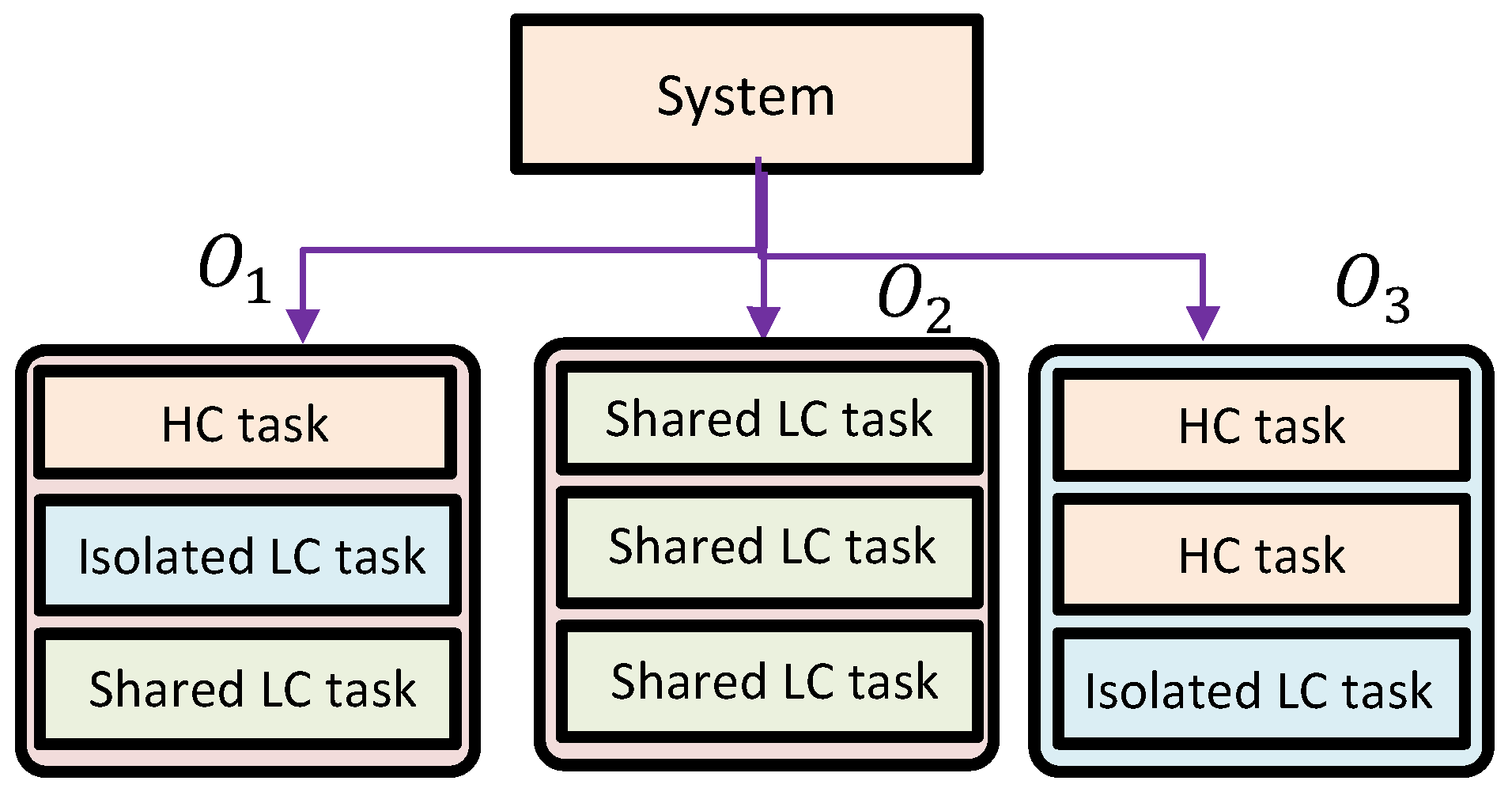
  • Component Model. As Figure 1 illustrates, we consider a component-based system with multiple MC components: S y s = def { O 1 , O 2 , , O j } . Each MC component O j is characterized by component interface I j and component workload W j , where W j is a set of tasks: W j = def { τ 1 , τ 2 , , τ i } .
  • Task Model. For simplicity, we consider dual criticality levels: HC and LC. We define an MC task model: task τ i is characterized by ( T i , C i L , C i H , χ i , ϕ i ) , where T i represents the minimum inter-job separation time, C i L is a low-criticality worst-case execution time (LO-WCET), C i H indicates a high-criticality WCET (HI-WCET), χ i is the task criticality level ( HC or LC ), and ϕ i denotes the isolation property ( true or false ). Task τ i has a relative deadline equal to T i . Given conservative assumptions for HI-WCETs, we assume that 0 < C i L C i H T i .
We can categorize each MC task depending on its parameter. An MC task is either LC or HC depending on its criticality level. An LC task is either isolated or shared depending on its isolation property. Component designers strive to protect a component’s isolated LC tasks from behavior outside the component.
We consider a sporadic task set τ = { τ i } , where task τ i represents a potentially infinite job release sequence. The LC and HC task sets are defined as τ L = def { τ i τ | χ i = LC } and τ H = def { τ i τ | χ i = HC } , respectively. The isolated and shared LC task set are defined as τ I = def { τ i τ L | ϕ i } and τ S = def { τ i τ L | ¬ ϕ i } , respectively.
Moreover, LC and HC task utilization values of task τ i are, respectively, defined as follows:
u i L = def C i L / T i   and u i H = def C i H / T i .
We define the collective task utilization values for HC and LC task sets, respectively, as follows:
U H L = def τ i τ H u i L , U H H = def τ i τ H u i H , U L L = def τ i τ L u i L , U I L = def τ i τ I u i L , and U S L = def τ i τ S u i L .
  • Behavior Model. We consider the behavioral model of HC and LC tasks in runtime scheduling. Each task τ i has a task mode (denoted as M i ) indicating its behavior. For HC tasks, we assume some degree of uncertainty about each job’s execution time. A job demonstrates LC behavior if the job completes within its LO-WCET or exhibits HC behavior otherwise. Task τ i is in LC mode ( M i = LC ) if it does not show HC behavior and in HC mode ( M i = HC ) otherwise.
When the job of an HC task yields HC behavior, the task changes its mode from LC to HC mode (called mode-switch), as illustrated in Figure 2a. We consider task-level mode-switch, where individual tasks change task modes independently. Each HC task initially starts in LC mode.
For LC tasks, we consider the execution mode that represents whether the task stopped executing (see Figure 2b): each LC task τ i exists in either an active or suspended mode ( M i = active or M i = suspended ). Initially, all LC tasks reside in active mode. At the mode-switch, the scheduler may suspend some LC tasks to schedule the mode-switching HC tasks whose execution requirement has changed from LO- to HI-WCET.
  • System Goal. In existing MC systems, MC schedulability is defined as follows: for a given MC task set, the system is MC-schedulable if
    • HC tasks are always schedulable, and
    • LC tasks are schedulable if no mode-switch occurs.
For component-based MC systems, we extend MC schedulability to a system with MC components:
Definition 1.
(Component-MC schedulability). A component is component-MC-schedulable if
  • Comp-MC-A: HC tasks are always schedulable;
  • Comp-MC-B: LC tasks are schedulable if no mode-switch occurs; and
  • Comp-MC-C: The schedulability of isolated LC tasks is unaffected by the behavior outside the component.
For a given system with MC components, the system is component-MC-schedulable if its every component is component-MC-schedulable.
In practice, it is typically crucial to maximize the performance of LC tasks while guaranteeing MC schedulability [11]. The system goal of component-based MC systems involves minimizing the suspension of LC tasks while guaranteeing component-MC schedulability.

2.2. Review of MC Scheduling Algorithms

Since the first paper on MC systems [12], numerous studies have been addressed for the MC domain (see [13] for details). Buruah et al. [14] considered the runtime system criticality mode where the system enters HC mode if some task executes for more than its LO-WCET. Earlier MC approaches [14,15,16] suspended all LC tasks at system-level HC mode, which is too pessimistic for LC functions of the system. Recent MC approaches [10,17,18,19,20] have adopted task-level criticality mode and achieved graceful degradation (suspending the minimal number of LC tasks at each task-level mode-switch).
To develop a new framework, we extended the existing MC adaptive scheduling (MC-ADAPT) [18] scheme (with a task-level criticality mode) into component environments. The MC-ADAPT suspends LC tasks selectively at each task-level mode-switch, whereas EDF-VD (earliest deadline first with virtual deadline) [15] suspends all LC tasks at the system-level mode-switch. With the selective suspension of the LC tasks, the MC-ADAPT can optimize LC task performance while achieving the same schedulability with EDF-VD. Further, MC-ADAPT achieves higher schedulability than EDF-VD with HC-mode-preferred tasks, indicating the HC tasks that demand resources in LC mode are larger than those in HC mode. HC-mode-preferred HC tasks start in HC mode, whereas other HC tasks start in LC mode.
The MC-ADAPT scheduling algorithm is summarized as follows:
(1)
Scheduling policy: Initially, all LC tasks start in active mode. All HC tasks except HC-mode-preferred tasks start in LC mode (HC-mode-preferred HC tasks are enforced to execute consistently in HC mode). The deadline-based scheduler assigns the highest priority to the task with the earliest effective deadline: For an HC task, the scheduler executes the task based on its VD if it is in LC mode and based on its real deadline otherwise. For an LC task, the scheduler executes the task based on its real deadlines.
(2)
Mode-switching algorithm: When an HC task mode-switches from LC to HC, the scheduler may suspend LC tasks due to the increased resource demand of the HC task (the increased upper bound of task execution time from LO-WCET to HI-WCET). Based on an online schedulability test (presented later), the scheduler chooses to suspend LC tasks.
The VD of task τ i is computed by V i = def x · T i , where x is the VD coefficient: x = def U H L / ( 1 U L L ) . Using the value of x, we can determine HC-mode-preferred tasks (requiring resource demands in LC mode larger than those in HC mode): τ F = def { τ i τ H | u i L / x > u i H } .
Before presenting the online schedulability test, we must define the system state to identify a different runtime state at a mode-switch.
Definition 2.
(System state). For a given task set τ, a system state S is defined as a four-tuple of disjoint sets: S = def ( τ H 1 , τ H 2 , τ L 1 , τ L 2 ) , where
  • τ H 1 : LC mode, HC task set ( τ H 1 = def { τ i τ H | M i = LC } ),
  • τ H 2 : HC mode, HC task set ( τ H 2 = def { τ i τ H | M i = HC } ) including the mode-switching task,
  • τ L 1 : active LC task set ( τ L 1 = def { τ i τ L | M i = active } ), and
  • τ L 2 : suspended LC task set ( τ L 2 = def { τ i τ L | M i = suspended } ) including LC tasks that are being suspended at a mode-switch.
The MC-ADAPT presents an online schedulability test that determines whether the system is schedulable with system state S at runtime:
U L 1 L + U H 1 L x + x · U L 2 L + U H 2 H 1 .
The MC-ADAPT also presents an offline schedulability analysis to determine whether a given system is MC-schedulable by MC-ADAPT. According to MC schedulability, the two different worst-case system states are the initial system state ( S ST ) and the worst-case system state after the mode-switch ( S MS ). When the system starts, the HC-mode-preferred tasks are in HC mode, the other HC tasks are in LC mode, and all LC tasks are released. Thus, we have S ST = ( τ H τ F , τ F , τ L , ) . After any mode-switch, we have S MS = ( , τ H , , τ L ) because all HC tasks are in HC mode and all LC tasks are suspended in the worst case. Then, we can derive the offline schedulability test: task set τ is MC-schedulable by MC-ADAPT if a real number x, such that 0 x 1 , satisfies both of the following conditions:
U L L + U H L x 1 ,
x · U L L + τ i τ H min ( u i L x , u i H ) 1 .

3. Component-Based Mixed-Criticality Scheduling Framework

We first present challenges and approaches (Section 3.1). Then, we present the process overview in Section 3.2. Finally, we present the CMC-DRA scheduling algorithm (Section 3.3) and CMC-DRA schedulability analysis (Section 3.4).

3.1. Challenges and Approaches

There are two challenges for systems with MC components. The first involves component resource allocation. Ren and Phan [9] statically allocated resources to isolate components. However, this static allocation leads to inefficient resource utilization. Overcoming the limitation, Gu et al. [10] adopted limited dynamic resource allocation, where resources are rearranged when the number of HC behaviors exceeds its TL. Nevertheless, component resources may differ depending on which tasks reveal HC behaviors. We require a fine-grained dynamic resource allocation method to improve resource efficiency further.
We consider dynamic resource allocation under component-/task-level criticality modes to address the challenge. Each task has a task-level criticality mode, indicating whether its execution time exceeds the LO-WCET estimate at runtime. Each component also has a component-level criticality mode, indicating whether the criticality mode of any task in the component is switched. Instead of static or limited dynamic resource allocation of components, we consider fully dynamic resource allocation to maximize resource efficiency.
The second challenge regards task scheduling inside a component. Even if we adopt dynamic resource allocation, naive scheduling algorithms cannot optimize system feasibility or the suspension of LC tasks. There are two possible approaches to task scheduling. Earlier MC scheduling approaches (e.g., AMC [14] and EDF-VD [15]) consider the runtime criticality mode (indicating whether HC behavior emerges at runtime) at the system level. After the system-level mode-switch, these approaches suspend all LC tasks, which impedes LC task performance. Recent MC scheduling approaches (e.g., Huang et al. [17], Gu et al. [10], and Lee et al. [18]) consider the runtime criticality mode at the task level. Among them, the MC-ADAPT scheme by Lee et al. [18] is a good candidate to schedule tasks in a component. Considering the runtime resource demand of HC tasks with the task-level criticality mode, the scheme suspends a subset of LC tasks.
We developed the proposed scheduling scheme in two steps to address the challenge. First, we extended the existing MC-ADAPT scheme [18] with flat component scheduling. In flat (non-hierarchical) scheduling, all tasks in all components are scheduled collectively by a single scheduler. Second, considering component isolation, we revised the mode-switching algorithm of MC-ADAPT because the direct application of MC-ADAPT cannot provide component isolation. We also considered that the external mode-switch could suspend the shared LC tasks for resource efficiency.

3.2. Process Overview

We propose CMC-DRA for component-based MC systems. Extending MC-ADAPT [18] with a flat scheduling policy, CMC-DRA does not separate component scheduling and task scheduling. In existing scheduling research, Gu et al. [10] and Lackorzynski et al. [21,22] adopted flat scheduling to improve resource efficiency on MC systems. In the aerospace industry, DEOS real-time operating systems [23] adopted a flat scheduling strategy.
In CMC-DRA, we introduce a component resource to separate the scheduling operations among components. For component O j , component resource Γ j R ( 0 Γ j 1 ), indicating the proportional share of the system resource. We have Γ j 1 for the uniprocessor system. For any time interval length t, a component O j with component resource Γ j receives up to Γ j · t time units of resources.
As the interface for component O j , we introduce I j = def { Γ j ST , Γ j EM , Γ j IM } , where Γ j ST is the initial component resource, Γ j EM denotes the component resource for the external mode-switch, and Γ j IM is the component resource for the internal mode-switch for O j . The system can use component interfaces to integrate components without considering internal component details. Section 3.4.2 presents the computation of the component interface and how to integrate components with component interfaces.
We can separate inter-component resource management and the intra-component mode-switching algorithm by introducing a component resource. The resource manager dynamically adjusts each component’s resources at the mode-switch. The mode-switching algorithm minimally suspends LC tasks at the mode-switch with a given component resource.
Schedulability analysis in standard MC systems does not apply directly to component-based MC systems. While simultaneous mode-switches are the worst-case scheduling scenario for standard MC systems, we do not know the worst-case scheduling scenario for component-based MC systems. We can compute each component’s required resources with only its internal runtime state. Using the component resource concept, we can independently analyze each component and combine the analysis results of components for system schedulability. Different component resource management affects the system schedulability differently.

3.3. The CMC-DRA Scheduling Algorithm

Extending the MC-ADAPT scheduling algorithm [18] to component environments, we propose a new scheduling algorithm for CMC-DRA. The basic scheduling policy of MC-ADAPT applies to CMC-DRA, including VD assignment. We present a new component resource manager and component-level mode-switching algorithm to support selective task suspension with component isolation. At a mode-switch, the component resource manager identifies the required component resource to handle the mode-switch. Then, the manager adjusts the component resources of all the components, including the mode-switching component. After the resources are adjusted for each component, the mode-switching algorithm suspends LC tasks selectively to schedule the component within the component resource.
Before presenting a component resource manager, we define the component state to identify different runtime task behaviors in a component, similar to the system state (Definition 2).
Definition 3.
(Component state). For a given component workload W j , the component state S j is defined as a four-tuple of disjoint sets: S j = def ( τ H 1 , j , τ H 2 , j , τ L 1 , j , τ L 2 , j ) , where τ X , j is τ X among W j .
Similar to the initial system state (Section 2.2), we define the initial component state as S j ST = ( τ H , j τ F , j , τ F , j , τ L , j , ) , where τ F , j indicates HC-mode-preferred HC tasks in W j .
Based on the component state (Definition 3), we present a component-level online schedulability test. The test is extended from Equation (1) in Section 2.2 with the component environment. For component O j , the test is defined for a given component state S j and component resource Γ j (the derivation is in Section 3.4):
U L 1 , j L + U H 1 , j L x + x · U L 2 , j L + U H 2 , j H Γ j .

3.3.1. CMC-DRA Component Resource Manager

The component resource manager dynamically adjusts all component resources and the remaining system resource (i.e., those unassigned to any component). Initially, each component is allocated with Γ j ST system resources. We let IdleRes be the remaining system resources. Then, we have IdleRes : = 1 Γ j ST . When a mode-switch in a component happens, it is assumed to be internal (Figure 3a). For an internal mode-switch, the resource manager must identify the mandatory and optional component resources to handle the mode-switch. Accordingly, we consider the current component state ( S j C ) after the mode-switch. In addition, ComputeMan ( S j C ) defines the mandatory component resources satisfying the component-MC schedulability. We confirm this by calculating the minimum component resource to satisfy Equation (4) when S j represents the transited component state by suspending all LC tasks from S j C . Moreover, ComputeOpt ( S j C ) indicates the optional component resources to reduce the suspension of LC tasks in O j :
ComputeOpt ( S j C ) = def Γ j C ComputeMan ( S j C ) ,
where Γ j C is the minimum component resource for the current component state S j C .
The detailed operations of the component resource manager are outlined as follows:
(1)
Mandatory resource adjustment: This step is vital to guarantee the component-MC schedulability of a component.
(a)
If the mandatory component resources ( ComputeMan ( S j C ) ) exceed the previously assigned component resource ( Γ j P ), we increase Γ j from Γ j P to ComputeMan ( S j C ) .
(b)
If the available resources ( Γ j P + IdleRes ) are smaller than the mandatory component resource, the mode-switch is changed to external (Figure 3b). For the external mode-switch, the component resource manager should request the component’s resource deficiency ( ReqRes ) from the system resource manager: ReqRes = def ComputeMan ( S j C ) ( Γ j P + IdleRes ) .
(2)
Optional resource adjustment (if IdleRes > 0 ): This step is optional to reduce the suspension of LC tasks. We increase Γ j by min ( ComputeOpt ( S j C ) , IdleRes ) .
The system resource manager is activated when component O j requests additional component resources ReqRes (>0):
(1)
Find a component O k s.t. O k O j and Γ k P > ComputeMan ( S k C ) .
(a)
O k can reduce its component resources from Γ k P to ComputeMan ( S k C ) . We let Γ k D be the maximum possible resource donation: Γ k D = def Γ k P ComputeMan ( S k C ) .
(b)
If ReqRes > Γ k D , we reduce the component resources of O k maximally and update ReqRes : = ReqRes Γ k D .
(c)
Otherwise, we reduce the component resources of O k only by ReqRes and update ReqRes : = 0 .
(2)
Repeat the above procedure until ReqRes = 0 . A feasible system passing the offline feasibility test (which will be presented in Section 3.4) must be terminated.

3.3.2. CMC-DRA Mode-Switching Algorithm

For a component, the mode-switching algorithm selects and suspends the active LC tasks when the component resources are reduced (by an external mode-switch) or when a mode-switch occurs in the component. Due to the reduced component resource budget or increased resource demand from the mode-switch, the component-level online schedulability test (Equation (4)) may not hold, meaning that HC tasks are no longer schedulable if the mode-switching algorithm is not activated. Then, to satisfy component-MC schedulability of the component, the mode-switching algorithm selectively suspends LC tasks until the online test holds.
The mode-switching algorithm may suspend LC tasks sufficiently to satisfy the online test (Equation (4)). Then, its component resources may be under-utilized after activating the mode-switching algorithm. The mode-switching algorithm collects these remaining component resources with the system-level parameter IdleRes . In a future mode-switch, CMC-DRA utilizes IdleRes to reduce the suspension of LC tasks (by providing optional resources).

3.4. Schedulability Analysis of CMC-DRA

We first present an online schedulability analysis to choose which LC tasks should be suspended for component-MC schedulability (inside components). Based on the online analysis, we present the offline feasibility analysis to determine whether a given component/system is schedulable by the CMC-DRA algorithm.

3.4.1. Online Schedulability Analysis

When an HC task mode-switches, its execution requirement changes from LO-WCET to HI-WCET, increasing the resource demand inside the component. Then, LC tasks may need to be suspended if the component resources are insufficient. An online schedulability analysis must check whether the component resources are sufficient. Component O j is said to be schedulable with component resource Γ j if, for any time interval of length t,
τ i W j DEM i ( t ) Γ j · t
where DEM i ( t ) is the resource demand of task τ i over t.
Extending Equation (1) in Section 2.2, we present a component-level online schedulability test to determine whether the component is schedulable with component resource Γ j and component state S j :
Theorem 1.
A component O j is schedulable with a given component resource Γ j and component state S j if Equation (4) holds.
The proof of Theorem 1 is presented in Appendix A, where its outline is similar to the proof of Theorem 5.3 in [18].

3.4.2. Offline Feasibility Analysis and Interface Computation

For a given system, offline feasibility indicates whether the system is schedulable by CMC-DRA in terms of component-MC schedulability. The system consists of components with their component interfaces. By checking component interfaces, we can determine the offline feasibility of the system. First, we present computation of the component interface for Γ j ST , Γ j EM , and Γ j IM . Next, we present the offline feasibility of the system, consisting of components with component interfaces.
For a given component O j , we compute the component interface I j = { Γ j ST , Γ j EM , Γ j IM } for three scenarios in component-MC schedulability (Definition 1 in Section 2.1): (1) no mode-switch occurs (comp-MC-A and comp-MC-B), (2) external mode-switches but no internal mode-switches occur (comp-MC-A and comp-MC-B), and (3) internal mode-switches occur (comp-MC-A). We can compute Γ j ST for scenario 1, Γ j EM for scenario 2, and Γ j IM for scenario 3. We can independently analyze each component and combine the analysis results of components for the system’s schedulability.
For each scenario, we identified the worst-case component state. For the first scenario, we have S j ST . Because S j ST = ( τ H , j τ F , j , τ F , j , τ L , j , ) , all LC tasks are in the active mode and all HC tasks are in the initial mode (HC mode for HC-mode-preferred tasks and LC mode otherwise). For the second scenario, we must identify S j EM (the worst component state when external mode-switches but no internal mode-switches occur). For the third scenario, we must identify S j IM (the worst component state when internal mode-switches occur).
After identifying the worst-case component states for the three scenarios, we can compute their minimum component resource demands. For S j ST , we can compute Γ j ST . For S j EM , we can compute Γ j EM , and for S j IM , we can compute Γ j IM .
The following lemma derives Γ j ST from the initial component state S j ST .
Lemma 1.
Consider a component O j and the initial component state S j ST . Then, O j is schedulable with a component resource Γ j if
Γ j Γ j ST = U L , j L + τ i τ H , j min ( u i L x , u i H ) .
Proof. 
Consider the initial component state S j ST = ( τ H , j τ F , j , τ F , j , τ L , j , ) . To illustrate that O j is schedulable, by Theorem 1, we must demonstrate that Equation (4) holds when S j = S j ST :
U L , j L + τ i τ H , j τ F , j u i L x + τ F , j u i H Γ j U L , j L + τ i τ H , j min ( u i L x , u i H ) Γ j , ( u i H < u i L x f o r τ i τ F , j )
which is true because Equation (5) holds. □
The following lemma derives Γ j EM for any component state when external mode-switches but no internal mode-switches occur.
Lemma 2.
Consider a component O j and any component state when external mode-switches but no internal mode-switch occur. Then, O j is schedulable with a component resource Γ j if
Γ j Γ j EM = U I , j L + x · U S , j L + τ i τ H , j min ( u i L x , u i H ) .
Proof. 
Consider S j EM , the worst-case component state for external mode-switches but no internal mode-switches. In S j EM , all shared LC tasks are in suspended mode (due to the external mode-switch). In S j EM , the isolated LC tasks should be in active mode and all the HC tasks should be in the initial mode because no internal mode-switches occur. To demonstrate that O j is schedulable, by Theorem 1 we must prove that Equation (4) holds when S j = S j EM :
U I , j L + x · U S , j L + τ i τ H , j min ( u i L x , u i H ) Γ j ,
which is true because Equation (6) holds. □
The following lemma derives Γ j IM for any component state when internal mode-switches occur.
Lemma 3.
Consider a component O j and any component state when internal mode-switches occur. Then, O j is schedulable with a component resource Γ j if
Γ j Γ j IM = x · U L , j L + U H , j H .
Proof. 
Consider S j IM , the worst-case component state for internal mode-switch. In S j IM , all LC tasks are suspended, and all HC tasks are in HC mode. To demonstrate that O j is schedulable, by Theorem 1 we must prove that Equation (4) holds when S j = S j IM :
x · U L , j L + U H , j H Γ j ,
which is true because Equation (7) holds. □
The following theorem derives the offline schedulability for a component by combining schedulability conditions for the three scenarios (Lemmas 1–3).
Theorem 2.
(Component schedulabilty). A component O j is component-MC-schedulable if Γ j Γ j ST when no mode-switch occurs, Γ j Γ j EM when external mode-switches but no internal mode-switches occur, and Γ j Γ j IM when internal mode-switches occur.
Proof. 
To satisfy component-MC schedulability, we must demonstrate that O j is schedulable in three different cases: (1) no mode-switch occurs (comp-MC-A and comp-MC-B), (2) external mode-switches but no internal mode-switches occur (comp-MC-A and comp-MC-B), and (3) internal mode-switches occur (comp-MC-A). For case 1, because Γ j Γ j ST , the component is schedulable by Lemma 1. For case 2, because Γ j Γ j EM , the component is schedulable by Lemma 2. For case 3, because Γ j Γ j IM , the component is schedulable by Lemma 3. □
Based on component schedulability, we present a theorem to determine the system feasibility (or system schedulability) for a given system with MC components. We assume that component interfaces are already computed in the system integration stage. Although three runtime scenarios (no mode-switches, external mode-switches but no internal mode-switches, and internal mode-switches) exist in component perspective, only two runtime scenarios (no mode-switches and mode-switches) exist in the system perspective because an internal mode-switch in one component is an external mode-switch in other components. Moreover, there does not exist only external mode-switches for all components. We must consider these runtime scenarios for a given system to check its feasibility.
Theorem 3.
(System feasibility). For a given system with MC components ( Sys = { O j } ), the system is component-MC-schedulable if Γ j ST 1 and max ( Γ j EM , Γ j IM ) 1 .
Proof. 
The maximum component resources under the uniprocessor platform is one (according to the definition of component resources in Section 3.2). We must consider two different scenarios. In the first system scenario, no mode-switches occur from any component. Then, by Theorem 2, the system is schedulable if Γ j ST 1 .
In the second system scenario, some mode-switches occur in some components. The existing mode-switches are external for components with no internal mode-switch. Then, we can determine the worst-case resource demand by comparing Γ j EM and Γ j IM of each component O j . Some components have Γ j EM Γ j IM , indicating that the components have the worst-case resource demand when external mode-switches occur but no internal mode-switches occur, and vice versa. Then, we can determine the worst-case system resource demand by max ( Γ j EM , Γ j IM ) . Thus, the system is schedulable if max ( Γ j EM , Γ j IM ) 1 by Theorem 2. □
The time complexity to check system feasibility is related with Lemmas 1–3 and Theorem 3. For component O j , interface computation (Lemmas 1–3) takes O ( k j ) where k j is the number of tasks in O j . When the number of components in Sys is m, the complexity to check Theorem 3 is O ( m ) . Then, the complexity to check system feasibility is O j Sys O ( k j ) + O ( m ) = O ( n ) , where n is the total number of tasks in any component of the system, i.e., O j Sys k j = n .

4. Evaluation

We evaluated the effectiveness of the CMC-DRA framework via extensive simulation. In Section 4.1, we present how to generate a synthetic workload for simulation. In Section 4.2, we present the simulation results.

4.1. Simulation Setup

To arrange a simulation, we generated random systems using the workload-generation algorithm [11,15,18], widely used in real-time systems. We let U b be the upper bound of system utilization in the LC and HC modes. A random component is generated with all task parameters being randomly drawn from a uniform distribution: for component O j ,
(1)
Component utilization, U j , is a real number drawn from the range [ 0.05 , 0.2 ] .
(2)
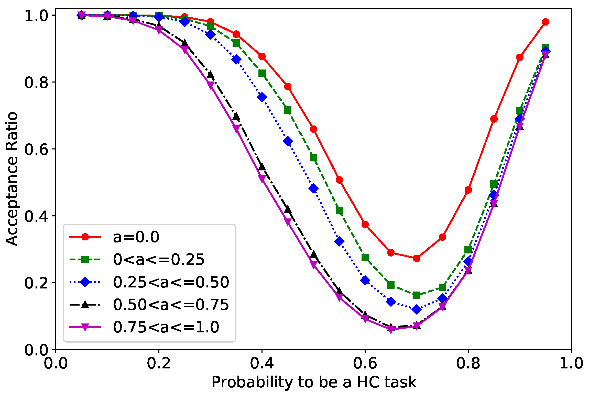
The ratio of isolated tasks over total LC tasks, α j , is a real number drawn from the range [ 0.25 , 0.75 ] .
(3)
For a task τ i ,
-
Task utilization, u i , is a real number drawn from the range [ 0.02 , 0.1 ] .
-
The ratio of u i H / u i L , R i , is a real number drawn from the range [ 1 , 4 ] .
-
The probability that the task is an HC task, P i , is a real number from the range [0, 1]. If P i < P HC (default value of P HC is 0.5), set χ i : = LC . Otherwise, set χ i : = HC .
(4)
We repeat the steps to generate a task in the component until max ( U j , H L + U j , L L , U j , H H ) exceeds U j . Then, we discard the task added last.
We repeat to generate a component until max ( U H L + U L L , U H H ) > U b 0.05 . If max ( U H L + U L L , U H H ) U b , the system is accepted. Otherwise, we discard the system, and generate a new system.
We used a desktop computer with an Intel i9-10900K 3.7 GHz processor with 32 GB RAM for the simulation environment. We implemented the simulation codes in the Java Standard Development Kit (v20.0.1).

4.2. Simulation Results

We evaluated CRC-DRA regarding system feasibility (using Theorem 3) for various scheduling algorithms and alpha parameters. We also evaluated CMC-DRA in terms of the deadline miss ratio.

4.2.1. System Feasibility for Scheduling Algorithms

To convey the effectiveness of the CMC-DRA scheduling algorithm, we compared CMC-DRA with two base-line scheduling algorithms for component MC systems:
(1)
A variant of the MC-ADAPT scheduling algorithm [18] for component-based systems: When a mode-switch occurs in a component, the algorithm selectively suspends LC tasks in the component. The mode-switch does not propagate to other components.
(2)
A variant of the EDF-VD scheduling algorithm [15] for component-based systems: When a mode-switch happens in a component, the algorithm suspends all LC tasks in the component. The mode-switch does not propagate to other components.
Figure 4 illustrates the acceptance ratio of CMC-DRA, MC-ADAPT, and EDF-VD with varying utilization bounds U b . Each data point draws from 5000 randomly-generated systems. As MC-ADAPT suspends LC tasks based on the global system state (not the component state), it may suspend the shared LC tasks in other components at a mode-switch. In the worst case, active isolated LC tasks still exist inside the component whose HC tasks are already mode-switched, decreasing the acceptance ratio. In the result, CMC-DRA yields up to 88.3% higher schedulability than EDF-VD, which offers low schedulability due to the complete component isolation. In addition, CMC-DRA has up to 63.5% higher schedulability than MC-ADAPT.

4.2.2. System Feasibility for Alpha Parameters

In Figure 5 and Figure 6, we investigated the effects of different alphas on the component-MC schedulability of CMC-DRA. Figure 5 displays the acceptance ratio of CMC-DRA varying the utilization bound U b (from 0.55 to 1.0 in steps of 0.05) with different alpha ranges ( α j = 0 , 0 < α j 0.25 , 0.25 < α j 0.50 , 0.50 < α j 0.75 , and 0.75 < α j 1 ). Specifically, we added the case of α j = 0 (no isolated task in any component), which is identical to existing MC scheduling approaches without considering each component. Furthermore, each component randomly picks α j within the given alpha range. Each data point draws from 5000 systems. As the utilization bound increases, the acceptance ratio decreases, incurring severe effects on larger α j . When α j = 0 , the CMC-DRA acceptance ratio is maximized due to no component isolation. As α j approaches 1, the acceptance ratio decreases because the degree of component isolation increases.
Figure 6 illustrates the acceptance ratio of CMC-DRA varying the probability to be an HC task ( P HC ) with different alpha ranges ( α j = 0 , 0 < α j 0.25 , 0.25 < α j 0.50 , 0.50 < α j 0.75 , and 0.75 < α j 1 ). Each data point draws from 5000 systems. Given an extremely high or low probability, the workload is close to a non-MC task set (solely HC or LC tasks). When we generate a task set for which HC or LC mode utilization is less than or equal to 1, the acceptance ratio is close to 1 as the task set matches the non-MC task set. Alternatively, as the probability nears 0.7, the acceptance ratio decreases, severely affecting alpha. We confirmed that the schedulability is worse when LC mode utilization and HC mode utilization are both high. This occurs when P HC is approximately 0.7, not 0.5: while generating an LC task increases only LC mode utilization, generating an HC task increases both HC mode and LC mode utilization (i.e., the increase in LC mode utilization depends on R i ). When P HC = 0.5 , the resulting system has higher LC mode utilization than HC mode utilization. When the number of HC tasks exceeds that of LC tasks ( P HC > 0.5 ), LC mode utilization and HC mode utilization are both high. There is a common observation for both Figure 5 and Figure 6: As α j increases, the acceptance ratio decreases, because the scheme reserves additional execution budgets to comply with the isolation requirement.

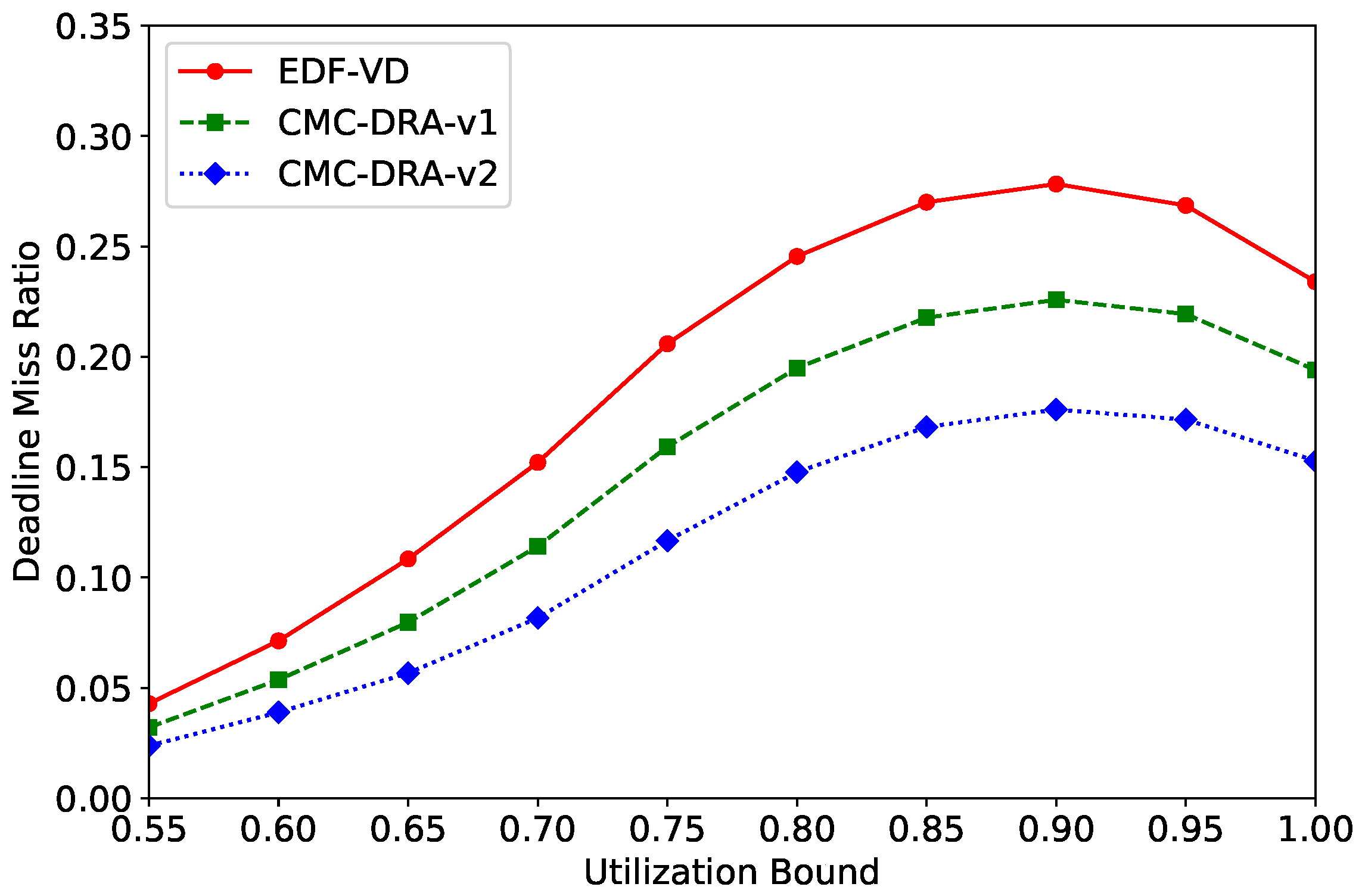
4.2.3. Runtime Performance (Deadline Miss Ratio of LC Tasks)

To evaluate the runtime performance of CMC-DRA, we compared the three approaches listed below (including CMC-DRA) in terms of the deadline miss ratio (DMR) of LC tasks:
(1)
The EDF-VD scheduling algorithm [15] is a non-component-based MC scheduling algorithm suspending all LC tasks at any mode-switch.
(2)
The CMC-DRA-v1 scheduling algorithm is a simplified version of the CMC-DRA algorithm without considering the component state and resource manager. At the mode-switch in a component, the algorithm suspends all LC tasks in the mode-switching component and suspends all shared LC tasks in other components.
(3)
The CMC-DRA-v2 scheduling algorithm is the proposed CMC-DRA algorithm, which strictly follows Section 3.3.
For a given randomly generated system with varying utilization bounds U b and 0.25 α j 0.75 , we simulate the behavior of tasks with a given probability to exhibit HC behavior ( P HB ) for 10,000 time units. We set P HB to 0.4. Each data point again draws from 5000 systems, and Figure 7 presents the simulation results. In the results, CMC-DRA-v1 and CMC-DRA-v2 reduced the DMR of EDF-VD by up to 26.5% and 47.7%, respectively, indicating that CMC-DRA offers improved service quality over the existing EDF-VD approach. Inside the CMC-DRA family, CMC-DRA-v2 reduced the DMR of CMC-DRA-v1 by up to 28.9%, which indicates that the CMC-DRA component resource manager (included in only CMC-DRA-v2) effectively reduces DMR. Table 1 describes the total simulation time over 45,000 workloads and the simulation time per workload for the three approaches. Since the runtime simulation time per each workload by the CRC-DRA algorithm for 10,000 time units was less than 17 ms, we confirmed that the CRA-DRA approach has a reasonable system overhead.

5. Discussion

5.1. Implementation in Autonomous Driving Mini Vehicles

To reflect the effectiveness of the proposed CMC-DRA framework, we may conduct case studies on autonomous driving vehicles. For example, F1TENTH [24] is an open-source autonomous driving racing platform with a one-tenth scale vehicle. We can implement the proposed CMC-DRA scheduler with multiple MC components, such as the front and side/back cameras. As investigated by Kang et al. [25], tasks for real-time object detection have different levels of criticality. We plan to evaluate the resource efficiency and control quality of CMC-DRA, compared to the existing framework.

5.2. Implementation with Virtualization Platforms

There have been many approaches to implementing real-time, component-based systems. Virtualization represents a promising architectural approach for component-based MC systems [26]. Specifically, container-based virtualization involves a light-weight alternative to hypervisor-based virtualization for component-based systems [4,27]. The proposed flat-hierarchical scheduling framework suits container-based virtualization well; thus, we may consider implementing the CMC-DRA framework on container-based virtualization in the future.

5.3. Limitations

The first limitation of CMC-DRA is that we only consider two levels of component-based systems. We must consider multi-level hierarchical component-based systems to apply CMC-DRA to general component-based systems. In future work, we can consider a system with multiple edge-level components where each edge-level component has multiple child components. Using the interface of the child component, we can compute the interface of an edge-level component. Then, we can check the system feasibility with the interfaces of edge-level components.
The second limitation of CMC-DRA is that we only consider the dual criticality system with HC and LC for simplicity. However, in practice, more than two criticality levels are used. In the automotive ISO 26262 standard [6], four levels of criticality are specified: ASIL (automotive safety integrity level) A (the lowest criticality), ASIL B, ASIL C, and ASIL D (the highest criticality). In future work, we aim to generalize the CMC-DRA framework into multiple levels of criticality. Then, we plan to introduce multiple WCET estimates for each MC task, similar to Vestal [12]. We may categorize an external mode-switch into mid-level external mode-switches (suspending the shared LC tasks) and high-level external mode-switches (suspending the shared mid-criticality and LC tasks).

6. Conclusions

Although component-based approaches reduce the complexity of designing CPSs, they incur resource inefficiency. The MC approaches can efficiently integrate components regarding resources but cannot have isolation properties among the components. A key challenge involves balancing component isolation and resource efficiency under component-based MC systems. To address this problem, we introduced the concept of component-MC schedulabilty, where the isolated tasks are protected from external mode-switches. Under the component-MC schedulability, we proposed a new CMC-DRA scheduling framework that suspends LC tasks selectively depending on the type of mode-switch (internal or external). Inside the framework, we present CMC-DRA scheduling algorithms with a component resource manager. We analyze online and offline schedulability for CMC-DRA. The simulation results prove that CMC-DRA yields up to 88.3% higher schedulability than EDF-VD and 63.5% higher schedulability than MC-ADAPT. In addition, CMC-DRA reduces DMR by up to 47.7% compared with existing work. The current CMC-DRC approach has limitations in that CMC-DRA only considers dual-criticality systems and two-level component-based systems. In the future, we plan to implement CMC-DRA on autonomous driving vehicles as a case study.

Author Contributions

Conceptualization, J.L. and K.K.; methodology, J.L.; software, J.L.; validation, J.L. and K.K.; formal analysis, J.L.; investigation, J.L.; resources, J.L.; data curation, J.L. and K.K.; writing—original draft preparation, J.L.; writing—review and editing, J.L. and K.K.; visualization, J.L.; supervision, J.L.; project administration, J.L.; funding acquisition, J.L. All authors have read and agreed to the published version of the manuscript.

Funding

This research was supported in part by Basic Science Program through the National Research Foundation of Korea (NRF), funded by the Minstry of Education (2022R1F1A1062660). In addition, it was supported in part by the MSIT (Ministry of Science and ICT), Korea, under the ITRC (Information Technology Research Center) support program (IITP-2023-2020-0-01655), supervised by the IITP (Institute of Information & Communications Technology Planning & Evaluation). This study was supported by the BK21 FOUR program (Education and Research Center for Securing Cyber-Physical Space) through the National Research Foundation (NRF) funded by the Ministry of Education of Korea (5199990314137).

Institutional Review Board Statement

Not applicable.

Informed Consent Statement

Not applicable.

Data Availability Statement

No new data were created or analyzed in this study. Simulation code is available in https://github.com/icpslab/mc_com (accessed on 29 April 2023).

Conflicts of Interest

The authors declare no conflict of interest.

Notation

The following notation is used in this manuscript:
O j An MC component
W j The workload of component O j (a set of tasks { τ i } )
τ i An MC task τ i =( T i , C i L , C i H , χ i , ϕ i )
T i Task period of τ i
C i L LO-WCET of τ i
C i H HI-WCET of τ i
χ i Task criticality of τ i ( H C or L C )
ϕ i Isolation property for LC tasks (true or false)
τ The set of tasks in all components in the system
τ H A set of tasks whose task criticality is H C : τ H = { τ i τ | χ i = HC }
τ L A set of tasks whose task criticality is L C : τ L = { τ i τ | χ i = LC }
τ I A set of LC tasks whose isolation property is true: τ I = { τ i τ L | ϕ i = true }
τ S A set of LC tasks whose isolation property is false: τ S = { τ i τ L | ϕ i = false }
M i Task mode of τ i indicating runtime task behavior
τ H 1 LC mode HC task set τ H 1 = { τ i τ H | M i = LC }
τ H 2 HC mode HC task set τ H 2 = { τ i τ H | M i = HC }
τ L 1 Active LC task set τ L 1 = { τ i τ L | M i = active }
τ L 2 Suspended LC task set τ L 2 = { τ i τ L | M i = suspended }
SSystem state indicating runtime state of the system: S = ( τ H 1 , τ H 2 , τ L 1 , τ L 2 )
xA system-wide virtual deadline tuning parameter
τ F HC-mode-preferred tasks τ F = { τ i τ H | u i L / x > u i H }
S j Component state indicating runtime state of component O j : S j = ( τ H 1 , j , τ H 2 , j , τ L 1 , j , τ L 2 , j )
S j C Current component state of O j
S j ST Initial component state of O j
S j EM The worst-case component state of O j when external mode-switches but no internal mode-switches occur
S j IM The worst-case component state of O j when internal mode-switches occur
Γ j Component resource indicating proportional share of the system resource for component O j
Γ j C The minimum component resource to schedule O j when S j = S j C
Γ j P The previously assigned component resource of O j
Γ j D The maximum possible resource donation of O j
Γ j ST The minimum component resource to schedule O j when S j = S j ST
Γ j EM The minimum component resource to schedule O j when S j = S j EM
Γ j IM The minimum component resource to schedule O j when S j = S j IM
DEM i ( t ) Resource demand of τ i over time interval length t
ComputeMan ( S j C ) The mandatory component resource to schedule O j for component-MC schedulability
ComputeOpt ( S j C ) The optional component resource to reduce the suspension of LC tasks in O j
IdleRes The remaining system resource that is not distributed to any component
ReqRes The deficiency of component resource to provide the mandatory component resource

Appendix A

To prove Theorem 1, we utilize a minimal instance of job release by W j that misses a deadline.
Proof of Theorem 1.
We will prove it by contradiction. Suppose that a deadline is missed. Let I denote a minimal instance of jobs released by W j on which a deadline is missed, and t 1 denote the time instant of the deadline miss. Let DEM ( t ) be an upper bound of the cumulative demand of all the tasks in the component over [ 0 , t ) . Since a deadline is missed at t 1 , we have DEM ( t 1 ) > Γ j · t 1 . To lead the contradiction, we will show that our calculation of DEM ( t 1 ) is no larger than Γ j · t 1 .
To compute DEM ( t 1 ) , we divide cases depending on whether the component state is the initial component state ( S j 0 = ( τ L , j , 0 , τ H , j τ F , j , τ F , j ) ) or not.
  • Case 1 ( S j is S j 0 ). We show that the collective demands over [ 0 , t 1 ) are equal to or less than Γ j · t 1 :
    DEM ( t 1 ) = τ i τ L , j DEM i ( t 1 ) + τ i τ H , j DEM i ( t 1 ) = ( τ i τ L , j u i L + τ i τ H , j u i L / x ) · t 1 ( b y   L e m m a   5 . 4   i n   [ 18 ] ) = ( U L , j L + U H , j L U F , j L x + U F , j H ) · t 1 ,
    which is equal to or less than Γ j · t 1 by Equation (4) with S j 0 .
  • Case 2 ( S j is not S j 0 ). Assume that the current component state S j is transited from a feasible component state S j P ( S j 0 is also a feasible system state) by one mode-switch. Let J * be the mode-switching job of task τ i before time t 1 and a * be the release time of J * . Let DEM i P ( t ) be DEM i ( t ) on S j P . Task τ q denotes the HC task which the latest mode-switching job before t 1 belongs to.
    We only need to show that the collective demands over [ 0 , t 1 ] are equal to or less than t 1 . Since S j P is a feasible component state, we have i DEM i P ( t ) Γ j · t for any t. We calculate the collective demand by dividing the cases depending on t 1 .
  • Case 2-A. ( t 1 a q * + x T q ). The collective demand is calculated as
    DEM ( t 1 ) = i DEM i ( t 1 ) i DEM i P ( t 1 ) ( b y   L e m m a   5 . 8   i n   [ 18 ] ) Γ j · t 1 . ( b y   t h e   a s s u m p t i o n o n   DEM i P )
  • Case 2-B. ( t 1 > a q * + x T q ). The collective demand is calculated as
    DEM ( t 1 ) = i DEM i ( t 1 ) i DEM i P ( a q * ) + ( t 1 a q * ) ( U L 1 , j L + U H 1 , j L x + x U L 2 , j L + U H 2 , j H ) ( b y   L e m m a   5 . 9   i n   [ 18 ] ) i DEM i P ( a q * ) + ( t 1 a q * ) Γ j ( b y   E q u a t i o n   ( 4 )   w i t h   S j ) Γ j · a q * + Γ j ( t 1 a q * ) ( b y   t h e   a s s u m p t i o n o n   DEM i P ) = Γ j · t 1 .
From Cases 2-A and 2-B, we showed that the collective demand is equal to or less than Γ j · t 1 . □

References

  1. Henzinger, T.; Matic, S. An Interface Algebra for Real-Time Components. In Proceedings of the 12th IEEE Real-Time and Embedded Technology and Applications Symposium (RTAS’06), San Jose, CA, USA, 4–7 April 2006; pp. 253–266. [Google Scholar] [CrossRef]
  2. Prisaznuk, P. Integrated modular avionics. In Proceedings of the Aerospace and Electronics Conference, NAECON 1992, Dayton, OH, USA, 18–22 May 1992; Volume 1, pp. 39–45. [Google Scholar] [CrossRef]
  3. ARINC653—An Avionics Standard for Safe, Partitioned Systems; Wind River Systems/IEEE Seminar. 2008. Available online: https://docplayer.net/287772-Arinc-653-an-avionics-standard-for-safe-partitioned-systems.html (accessed on 20 February 2023).
  4. Abeni, L.; Balsini, A.; Cucinotta, T. Container-Based Real-Time Scheduling in the Linux Kernel. SIGBED Rev. 2019, 16, 33–38. [Google Scholar] [CrossRef]
  5. Cucinotta, T.; Abeni, L.; Marinoni, M.; Balsini, A.; Vitucci, C. Reducing Temporal Interference in Private Clouds through Real-Time Containers. In Proceedings of the 2019 IEEE International Conference on Edge Computing (EDGE), Milan, Italy, 8–13 July 2019; IEEE Computer Society: Los Alamitos, CA, USA, 2019; pp. 124–131. [Google Scholar] [CrossRef]
  6. ISO/DIS 26262-1; Road Vehicles Functional Safety Part 1 Glossary. Technical Report; ISO: Geneva, Switzerland, 2009.
  7. Gall, H. Functional safety IEC 61508/IEC 61511 the impact to certification and the user. In Proceedings of the AICCSA, IEEE Computer Society, Doha, Qatar, 31 March–4 April 2008; pp. 1027–1031. [Google Scholar]
  8. AUTOSAR. AUTomotive Open System Architecture. Available online: www.autosar.org (accessed on 29 April 2023).
  9. Ren, J.; Phan, L.T.X. Mixed-Criticality Scheduling on Multiprocessors Using Task Grouping. In Proceedings of the 2015 27th Euromicro Conference on Real-Time Systems (ECRTS), Lund, Sweden, 8–10 July 2015; pp. 25–34. [Google Scholar] [CrossRef]
  10. Gu, X.; Easwaran, A.; Phan, K.M.; Shin, I. Resource Efficient Isolation Mechanisms in Mixed-Criticality Scheduling. In Proceedings of the 2015 27th Euromicro Conference on Real-Time Systems (ECRTS), Lund, Sweden, 8–10 July 2015; pp. 13–24. [Google Scholar] [CrossRef]
  11. Burns, A.; Baruah, S. Towards A More Practical Model for Mixed Criticality Systems. In Proceedings of the First Workshop of Mixed Criticality Systems (WMC 2013), Vancouver, BC, Canada, 3–6 December 2013; pp. 1–6. [Google Scholar]
  12. Vestal, S. Preemptive Scheduling of Multi-criticality Systems with Varying Degrees of Execution Time Assurance. In Proceedings of the 28th IEEE International Real-Time Systems Symposium, RTSS 2007, Tucson, AZ, USA, 3–6 December 2007; pp. 239–243. [Google Scholar] [CrossRef]
  13. Burns, A.; Davis, R.I. A Survey of Research into Mixed Criticality Systems. ACM Comput. Surv. 2017, 50, 1–37. [Google Scholar] [CrossRef]
  14. Baruah, S.; Burns, A.; Davis, R. Response-Time Analysis for Mixed Criticality Systems. In Proceedings of the 2011 IEEE 32nd Real-Time Systems Symposium (RTSS), Vienna, Austria, 29 November–2 December 2011; pp. 34–43. [Google Scholar] [CrossRef]
  15. Baruah, S.; Bonifaci, V.; D’Angelo, G.; Li, H.; Marchetti-Spaccamela, A.; van der Ster, S.; Stougie, L. The Preemptive Uniprocessor Scheduling of Mixed-Criticality Implicit-Deadline Sporadic Task Systems. In Proceedings of the 2012 24th Euromicro Conference on Real-Time Systems (ECRTS), Pisa, Italy, 11–13 July 2012; pp. 145–154. [Google Scholar]
  16. Guan, N.; Ekberg, P.; Stigge, M.; Yi, W. Effective and Efficient Scheduling of Certifiable Mixed-Criticality Sporadic Task Systems. In Proceedings of the 2011 IEEE 32nd Real-Time Systems Symposium (RTSS), Vienna, Austria, 29 November–2 December 2011; pp. 13–23. [Google Scholar] [CrossRef]
  17. Huang, P.; Kumar, P.; Stoimenov, N.; Thiele, L. Interference Constraint Graph—A new specification for mixed-criticality systems. In Proceedings of the 2013 IEEE 18th Conference on Emerging Technologies Factory Automation (ETFA), Cagliari, Italy, 10–13 September 2013; pp. 1–8. [Google Scholar] [CrossRef]
  18. Lee, J.; Chwa, H.S.; Phan, L.T.X.; Shin, I.; Lee, I. MC-ADAPT: Adaptive Task Dropping in Mixed-Criticality Scheduling. ACM Trans. Embed. Comput. Syst. 2017, 16, 163:1–163:21. [Google Scholar] [CrossRef]
  19. Chen, G.; Guan, N.; Hu, B.; Yi, W. EDF-VD Scheduling of Flexible Mixed-Criticality System with Multiple-Shot Transitions. IEEE Trans.-Comput.-Aided Des. Integr. Circuits Syst. 2018, 37, 2393–2403. [Google Scholar] [CrossRef]
  20. Lee, J.; Lee, J. MC-FLEX: Flexible Mixed-Criticality Real-Time Scheduling by Task-Level Mode Switch. IEEE Trans. Comput. 2022, 71, 1889–1902. [Google Scholar] [CrossRef]
  21. Lackorzyński, A.; Warg, A.; Völp, M.; Härtig, H. Flattening Hierarchical Scheduling. In Proceedings of the Tenth ACM International Conference on Embedded Software; EMSOFT’12. ACM: New York, NY, USA, 2012; pp. 93–102. [Google Scholar] [CrossRef]
  22. Lackorzynski, A.; Völp, M.; Warg, A. Flat but Trustworthy: Security Aspects in Flattened Hierarchical Scheduling. SIGBED Rev. 2014, 11, 8–12. [Google Scholar] [CrossRef]
  23. Deos: A Time & Space Partitioned DO-178 Level A Certifiable RTOS. Available online: http://www.ddci.com/products_deos.php (accessed on 29 April 2023).
  24. O’Kelly, M.; Zheng, H.; Karthik, D.; Mangharam, R. F1TENTH: An Open-source Evaluation Environment for Continuous Control and Reinforcement Learning. In Proceedings of the NeurIPS 2019 Competition and Demonstration Track; Escalante, H.J., Hadsell, R., Eds.; PMLR: Vancouver, BC, Canada, 2020; Volume 123, pp. 77–89. [Google Scholar]
  25. Kang, W.; Chung, S.; Kim, J.Y.; Lee, Y.; Lee, K.; Lee, J.; Shin, K.G.; Chwa, H.S. DNN-SAM: Split-and-Merge DNN Execution for Real-Time Object Detection. In Proceedings of the 2022 IEEE 28th Real-Time and Embedded Technology and Applications Symposium (RTAS), Milano, Italy, 4–6 May 2022; pp. 160–172. [Google Scholar] [CrossRef]
  26. Cinque, M.; Cotroneo, D.; De Simone, L.; Rosiello, S. Virtualizing mixed-criticality systems: A survey on industrial trends and issues. Future Gener. Comput. Syst. 2022, 129, 315–330. [Google Scholar] [CrossRef]
  27. Struhár, V.; Behnam, M.; Ashjaei, M.; Papadopoulos, A.V. Real-Time Containers: A Survey. In Proceedings of the 2nd Workshop on Fog Computing and the IoT (Fog-IoT 2020); Cervin, A., Yang, Y., Eds.; Schloss Dagstuhl–Leibniz-Zentrum fuer Informatik: Dagstuhl, Germany, 2020; Volume 80, pp. 7:1–7:9. [Google Scholar] [CrossRef]
Figure 1. The hierarchy of components and tasks: a system consists of multiple MC components ( O 1 , O 2 , ⋯); an MC component consists of HC tasks, the shared LC tasks, and the isolated LC tasks.
Systems 11 00281 g001
Figure 2. The behavioral model of tasks: an HC task initially starts in LC mode, and switches to HC mode when it executes more than LO-WCET ( C i L ); an LC task initially starts in the active mode (executing up to LO-WCET ( C i L )), and is suspended by a scheduling decision at a mode-switch of some HC task.
Systems 11 00281 g002
Figure 3. Mode-switch in CMC-DRA. (a) Internal mode-switch affects only LC tasks inside the component. (b) A mode-switch is changed to be external if the required resource demand is not satisfied, even if all internal LC tasks are suspended. Then, the external mode-switch affects internal LC tasks and the shared LC tasks in other components.
Systems 11 00281 g003
Figure 4. System feasibility for CMC-DRA, MC-ADAPT [18], and EDF-VD [15].
Systems 11 00281 g004
Figure 5. System feasibility of CMC-DRA varying utilization bound for different alpha parameters.
Systems 11 00281 g005
Figure 6. System feasibility of CMC-DRA varying the probability to be an HC task ( P HC ) for different alpha parameters.
Systems 11 00281 g006
Figure 7. Runtime Performance (Deadline Miss Ratio of LC tasks) for EDF-VD [15], CMC-DRA-v1, and CMC-DRA-v2.
Systems 11 00281 g007
Table 1. Simulation time for runtime performance.
EDF-VDCMC-DRA-v1CMC-DRA-v2
Total simulation time737,419 ms769,343 ms731,906 ms
Simulation time per each workload16.387 ms17.097 ms16.265 ms
Disclaimer/Publisher’s Note: The statements, opinions and data contained in all publications are solely those of the individual author(s) and contributor(s) and not of MDPI and/or the editor(s). MDPI and/or the editor(s) disclaim responsibility for any injury to people or property resulting from any ideas, methods, instructions or products referred to in the content.

