Abstract
To overcome the limitations of the present grey models in spatial data analysis, a spatial weight matrix is incorporated into the grey discrete model to create the SDGM(1,1,m) model, and the L1-SDGM(1,1,m) model is proposed, considering the time lag effect to realize the simultaneous forecasting of spatial data. The validation of the SDGM(1,1,m) and L1-SDGM(1,1,m) models is achieved, and finally, the per capita energy consumption levels (PCECs) of 30 provinces in China from 2020 to 2025 is predicted using SDGM(1,1,m) with a metabolic mechanism. We draw the following conclusions. First, the SDGM(1,1,m) and L1-SDGM(1,1,m) models established in this paper are reasonable and improve forecasting accuracy while supporting interactive regional forecasting. Second, although SDGM(1,1,m) resembles the DGM(1,n) model, their modeling conditions and targets are different. Third, the SDGM(1,1,m) and L1-SDGM(1,1,m) models can be used to effectively analyze the spatial spillover effects within the selected modeling interval while achieving accurate predictions; notably, from 2010 to 2017, the PCECs of Inner Mongolia and Qinghai were most affected by spatial factors, while the PCECs of Jilin, Jiangxi, and other provinces were influenced little by spatial factors. Fourth, predictions indicate that the PCECs of most Chinese provinces will increase under the current grey conditions, while the PCECs of provinces such as Beijing are expected to decrease.
1. Introduction
Recently, China’s economy has grown rapidly, with energy consumption subsequently increasing. According to the China Energy Statistical Yearbook, China’s total energy consumption rose from 1.5 billion tons of standard coal in 2000 to 4.9 billion tons of standard coal in 2019. In 2019, China’s external energy dependence was 21%, including 70.8% for crude oil, which exceeded the alert threshold of 50%, and the energy shortage is becoming increasingly serious. In the face of a growing energy demand, energy imports continue to increase, which has become a potential obstacle to sustainable development. Additionally, China’s 14th Five-Year Plan proposes to reduce the energy consumption per unit of GDP by 13.5% by 2025 and CO2 emissions by 18% compared to the respective level in 2020. In this context, a reasonable forecast of China’s future energy consumption is of high practical significance for ensuring energy security and formulating energy conservation policies.
There are many methods for forecasting energy consumption, and three major categories can be distinguished. The first category contains statistical analysis models, such as the autoregressive integrated moving average (ARIMA) [1,2,3], time series analysis [4,5], multiple linear regression [6], exponential smoothing [7], and Bayesian theory [8] models. The second category encompasses artificial intelligence methods, including artificial neural networks (ANNs) [9,10], support vector machines (SVMs) [11], and BP neural networks [12]. The third category involves grey models. There are certain differences between grey models and the above two types of models. The above two types of models are mostly white system models, that is, full information models, which need to consider all factors related to system operation and require large sample sizes. The prediction accuracy of these models is reduced if information is inaccurate or if the sample size is insufficient. However, in practice, it is often difficult to obtain a large amount of original sample data due to the difficulty of data collection and potentially low observation accuracy, and it is unrealistic for all information to be known, thus limiting the accuracy of prediction in various cases. In contrast, a grey model can model a system with only some known information, and it can be used to predict energy consumption without considering various factors, thereby overcoming the uncertainty problems associated with small sample sizes. As grey forecasting models are easy to use, simple, and accurate, they are broadly utilized for predicting energy consumption [13,14,15,16,17,18].
Grey systems are the main components of grey theory [19]. A grey system is a system that is neither white nor black; that is, the available information is incomplete. Grey predictive models combine grey system theory and other concepts, and there is a growing variety of grey models which can be broadly divided into univariate and multivariate model classes. In univariate models, one variable is studied, and other influencing factors are ignored. Multivariate grey models are based on a dependent variable and multiple independent variables, model the effects of various factors, and are classic causal forecasting models. Recently, grey forecasting models have been increasingly optimized and improved from various perspectives, such as background value optimization [20,21], fractional order accumulation and opposite direction accumulation [22,23,24], data preprocessing [25,26], model parameter optimization [27,28,29], model structure extension [30,31], information prioritization, and rolling prediction [32,33,34,35]. To encompass the advantages of grey models with those of other forecasting models, combined models have been developed [36,37]. In addition to broadening the basic structures, optimized grey models enhance forecasting performance and adaptability and are broadly used in numerous domains, such as in studies of carbon emissions [38,39], environmental sustainability performance [40], the consumption of petroleum products [41], traffic signal control [42], and COVID-19 [43].
It is worth discussing the emergence of discrete grey models. The derivation calculation required for the traditional grey model involves a direct switch from a discrete to a continuous form, which can lead to background value error and parameter estimation error in the modeling process. To solve this problem, Xie and Liu [44] proposed the discrete grey model, DGM(1,1), the basic form of which is a first-order difference equation that eliminates the discretization error of the GM(1,1) model. Therefore, DGM(1,1) is better suited to describing the development pattern of a system than GM(1,1). On this basis, scholars have conducted research on discrete grey models, and a large number of new discrete grey models have emerged: NDGM(1,1) [45], RDGM(1,n) [46], CDGM(1,1) [47], DGPM(1,1,N) [48], ATDGM(1,1) [49], WFDPGM(1,1,) [50], FDGM(1,1,,) [51], and DTDGM(1,N,) [52], among others.
Overall, scholars have made significant improvements to grey models from multiple perspectives, but energy consumption forecasting still requires improvement. Currently, grey models are primarily used for modeling time sequences and are not capable of modeling panel data or associations among spatial data, particularly for predicting energy consumption. Notably, they generally fail to consider the spatial correlations among energy consumption characteristics in different regions. Based on existing research, energy consumption displays spatial correlations [53,54,55,56,57]. Therefore, the consideration of spatial correlations is useful when forecasting energy consumption and analyzing geospatial relationships.
To overcome the limitations of the present grey models, based on the superiority of discrete models, spatial interaction is incorporated into DGM(1,1), thereby building the spatial discrete grey prediction model SDGM(1,1,m) for the associative forecasting of spatial data. Second, L1-SDGM(1,1,m) is established since spatial interaction processes are often accompanied by time lag effects. Finally, the validities of the SDGM(1,1,m) and L1-SDGM(1,1,m) models are verified based on PCEC data from 30 provinces in China, and the PCECs of the 30 provinces are forecasted from 2020 to 2025 using SDGM(1,1,m) with a metabolic mechanism. The contributions of this study are as follows:
- (1)
- In this paper, spatial characteristics are incorporated into DGM(1,1), which enhances spatial data predictions. SDGM(1,1,m) is proposed and is used to analyze spatial spillover effects in the selected modeling interval, and a grey model is used to process panel data.
- (2)
- SDGM(1,1,m) is compared with DGM(1,n), and the differences between them are analyzed in terms of modeling purposes and requirements.
- (3)
- In this paper, considering the time lag effect that often accompanies spatial interaction processes, L1-SDGM(1,1,m) is proposed, thus providing a conceptual approach for establishing other time-lag-based spatial discrete grey models.
- (4)
- Using the PCEC data from 30 provinces in China, SDGM(1,1,m) and L1-SDGM(1,1,m) are compared with DGM(1,1), DGM(1,n), NDGM(1,1), and BP neural network models to verify the effectiveness and superiority of SDGM(1,1,m) and L1-SDGM(1,1,m) for predicting the PCEC of China.
- (5)
- Based on a metabolic concept, we use SDGM(1,1,m) to predict the PCECs of 30 provinces in China from 2020–2025.
This study is organized as follows. In Section 2, DGM(1,1) is presented, the SDGM(1,1,m) model with spatial spillover terms is constructed, and the L1-SDGM(1,1,m) model with time lag effects is established. In Section 3, the validities of the SDGM(1,1,m) and L1-SDGM(1,1,m) models are verified with PCEC data from 30 provinces, and the PCECs of these regions are predicted for 2020–2025. Section 4 provides the conclusions of the study.
2. Construction of SDGM(1,1,m) and L1-SDGM(1,1,m)
2.1. Introduction of DGM(1,1)
For the input , denotes transposition. The corresponding first-order cumulative sequence (1-AGO) is , where
Then,
Which is said to be the basic form of DGM(1,1). is obtained using the formula below:
where , , and denote the estimated values and all obtained values below represent estimates.
According to Equation (2), we can obtain the corresponding ultimate simplified equation from the difference equation and cumulative reduction.
2.2. Definition of SDGM(1,1,m)
According to the theory of spatial characteristics, the variables in a certain region are positively or negatively influenced by the characteristic variables in surrounding regions, which suggests that the spatial spillover effect caused by spatial correlation plays an important role in influencing economic indicators [58]. Therefore, when predicting the future trend of a regional characteristic variable, it is necessary to consider not only the inertial influence of the regional characteristic variable but also the spatial influence of the neighboring regional characteristic variables. Therefore, the introduction of spatial correlation into a grey model can enhance the modeling approach.
Definition 1.
Suppose the input data for a model are , where and , with denoting the number of regions and denoting the periods considered. The raw sequence of the th region can be represented as . The data from all spatial cells at time are represented as , where is the transpose symbol. The first-order accumulation of is , where
Then,
If there is a spatial correlation between the variables, then
Which is said to be the basic form of the spatial discrete grey model SDGM(1,1,m), where refers to the interaction among different regions, i.e., the spatial lag term for the sequence , and is a spatial matrix with values of 0 along the main diagonal and a symmetric form.
Let , with denoting the first-order accumulation of ; this calculation is then implemented based on Equation (8). Consequently, it is easy to see that:
Then, Equation (9) is written as
The equation can be converted into the following difference equations:
Referring to Equation (3), in the th equation is estimated according to the least-squares method:
where
Reorganizing Equation (9) yields:
where is denoted as the unit matrix of . Through the equations above, we can obtain:
Referring to Equation (8), the ultimate simplified equation can be established as:
Given the description of SDGM(1,1,m), first, after introducing the relevant spatial characteristics into DGM(1,1), the joint forecasting of multiple spatial variables can be achieved, thus solving the problem that the traditional grey model is insufficient for spatial or panel data and creating a bridge between the grey model and spatial observation data. Second, the spatial correlation is treated as a control variable, and adding more control variables theoretically improves the model’s accuracy. Third, through parameter estimation, the spatial correlation coefficient matrix can be calculated, which allows simple analyses of spillover effects to be performed for each spatial unit in the modeling period. With this approach, spatial spillover effects can be analyzed, and the complex spatial structures that are prevalent in the spatial economic system can be assessed.
Additionally, Equation (13) can be written as
In addition, the basic form of the multivariate discrete grey model DGM(1,n) is:
As shown above, SDGM(1,1,m) is very similar in form to DGM(1,n), but they are different in terms of modeling conditions, targets, and the economic implications they represent. In SDGM(1,1,m), panel data are used, but time sequences are used in DGM(1,n). Additionally, spatial correlations among variables are required in SDGM(1,1,m), but causality or correlations among different variables are required in DGM(1,n). Multiple regions are modeled together in SDGM(1,1,m) to improve forecasting performance, while the causality among variables is used in DGM(1, n) to obtain predictions of multiple variables.
2.3. Definition of L1-SDGM(1,1,m)
The spatial spillover effect is usually accompanied by time dependence, i.e., there is a time lag in the influence of spillover effects on variables, and the SDGM(1,1,m) model does not consider this lag factor. Since the interval of time lag effects can vary, spatial grey models that consider time lag also differ. In this paper, we establish the spatial discrete grey model, L1-SDGM(1,1,m), with one time lag interval; other lag models can be developed based on this method and will not be discussed in detail in this paper.
Definition 2.
Let and be expressed as in Definition 1; then,
is said to be L1-SDGM(1,1,m), where L denotes lag. The matrices are as stated in Definition 1. Additionally, the matrix is as stated in Definition 1. Then, the above model is also converted into the following difference equations:
Referring to Equation (3), in the th equation can be estimated as follows:
where
Suppose the matrix satisfies:
Then, the model is written as
The time response equation and ultimate simplified equation are calculated from the equations above:
2.4. Error Evaluation Index
To verify the reliability and fit of both SDGM(1,1,m) and L1-SDGM(1,1,m), the accuracy of each model is assessed based on the mean absolute percentage error (MAPE). The traditional MAPE is often used for evaluating the forecasting results for a region, and it is very complex to use the MAPE to evaluate the forecasting results of multiple regions. Thus, this metric is improved here. Since the original sequence should be divided into simulation and prediction sets, the simulation, prediction, and total errors are computed separately as they can be expressed as the mean relative percentage error of simulation (MRPES), mean relative percentage error of forecasting (MRPEF), and the combined mean relative percentage error (CMRPE). The corresponding formulas are as follows:
where is the modeling interval and is the prediction interval. In general, the prediction performance is considered sufficient when the error is less than 8%, good when the error is less than 5%, and excellent when the error is less than 1%. In addition, to better compare the model performance, the RMSPE, RMSE, MAE, IA, and R are used as evaluation metrics for comparison, and they are calculated as shown in Table 1.

Table 1.
Evaluation metrics.
2.5. Flow Chart of SDGM(1,1,m)
The operation process of SDGM(1,1, m) is illustrated in Figure 1.
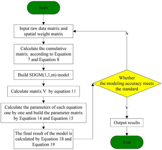
Figure 1.
Flowchart of the SDGM(1,1,m) model.
3. Applications in Forecasting PCEC in China
First, the PCEC data for 30 provinces in mainland China are introduced. Second, a spatial weight matrix is established, and the ESDA method is used to assess the spatial correlations among the PCEC trends in the 30 Chinese provinces. Third, PCEC data from China are used for model comparison. Finally, the PCECs of 30 Chinese provinces from 2020–2025 are forecasted using SDGM(1,1,m).
3.1. Data Collection
PCEC data from 30 Chinese provinces were obtained by dividing the total energy consumption by the number of people in each province, as follows.
where the subscript is the ID number of the province, and indicates the year. The energy consumption data and the population data are from the China Statistical Yearbook (stats.gov.cn, accessed on 5 February 2023).
The PCEC data from 2010 to 2019 can be obtained based on the above formula, as shown in Figure 2. The PCECs of each province in China in 2019 are shown in Figure 3. From the curves of the PCECs of each region, 28 provinces, excluding Beijing and Henan, experienced increased PCECs in 2019 compared with the level in 2010. Additionally, 28 provinces, excluding Henan and Tianjin, experienced increased PCECs after 2015. Moreover, the PCEC curves of geographically close provinces, such as those of Liaoning, Jilin, and Heilong, are similar, with increases before 2012, decreases from 2012 to 2015 and increases after 2015. The PCEC curves of five regions, Jiangsu, Zhejiang, Anhui, Fujian, and Jiangxi, all approximate a rising straight line. The curves for Hunan, Hubei, Chongqing, Sichuan, and Guizhou display the same shape and decrease and increase at the same times. The curves for Shaanxi, Gansu, Qinghai, Ningxia, and Xinjiang are also similar, with an upward trend. This phenomenon reflects the spatial correlation of the PCEC to some extent. As shown in Figure 3, in 2019, the PCECs of the northern and coastal regions of China were high, and Inner Mongolia, Qinghai, and Xinjiang displayed the highest PCECs; additionally, the PCECs were moderate in coastal regions such as Shandong, Jiangsu, Zhejiang, and Fujian, and the PCECs of southern regions such as Hunan, Hubei, Sichuan, and Chongqing were low. Thus, the PCECs were similar among neighboring regions, reflecting certain spatial correlation characteristics.
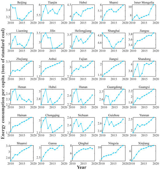
Figure 2.
PCEC data in China.
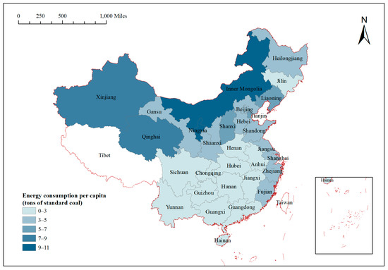
Figure 3.
Spatial distribution of PCECs in 2019.
Based on the PCECs of each province over time, the overall PCEC displays an upward trend overall, but there are differences among provinces. For instance, the PCEC of Henan decreases, the PCECs of Beijing and Tianjin decrease in the early stage and increases in the later stage, and the PCEC curve in Tianjin exhibits large fluctuations. Consequently, building an appropriate model for PCEC forecasting in these 30 provinces is a significant challenge.
3.2. Establishment of the Spatial Weight Matrix
In this paper, spatial correlation is incorporated into the discrete grey model through the spatial weight matrix, and the SDGM(1,1,m) model is constructed. Therefore, it is necessary to determine whether there are spatial correlation trends in the PCEC of China before further modeling is conducted. In this paper, we use Moran’s I index from the ESDA to assess the spatial correlations of the PCEC. It is necessary to establish a matrix prior to correlation testing. Therefore, referring to the practice of Wang and Zhang [59], we select a spatial geographic matrix to model, and the specific settings are shown below.
where denotes the geographical distance between provinces and , indicating that the interaction intensity of the energy consumption between the two provinces is inversely proportional to the distance between them.
From Table 2, we can see that Moran’s I value is significantly higher than 0 every year from 2010 to 2019, which indicates that the PCECs are significantly positively correlated among provinces; additionally, the overall PCEC displays high–high or low–low clustering trends, which are consistent with the spatial characteristics of the PCECs in Section 3.1. Therefore, to predict the PCEC, spatial correlation can be introduced into the grey prediction model.
Table 2.
Global Moran’s I values for PCECs from 2010 to 2019.
3.3. Model Comparison
To verify the validities of the SDGM(1,1,m) and L1-SDGM(1,1,m) models, according to the approach described in the previous section, the new model is built by improving DGM(1,1) and is similar to the DGM(1,n) model; therefore, the DGM(1,1) and DGM(1,n) models are selected for comparison. In addition, we choose the NDGM(1,1) and BP models as benchmark models for comparison. Among them, the DGM(1,1), NDGM(1,1), and BP models are separately used for each region. The PCECs of each region are modeled with different variables in DGM(1,n). In the following discussion, the abbreviations of these five models are simplified as SDGM, L1-SDGM, DGM, MDGM, NDGM, and BP. Since SDGM(1,1,m) and L1-SDGM(1,1,m) require the use of a spatial weight matrix, Equation (33) is again used for modeling.
In this paper, six models are applied using PCEC data from 30 Chinese provinces from 2010 to 2017, and the PCEC from 2018 to 2019 is predicted. Table 3 lists the errors of all models; notably, the modeling error of MDGM is very high, and the model completely fails to predict the PCECs of the 30 regions of China considered. As stated earlier, MDGM is a causal model based on causality or correlations among different variables; however, in this example, the PCECs of different regions are not related by causality, so the error of the MDGM model is particularly large. The errors of the SDGM and L1-SDGM models are less than 8% in both the simulation and prediction stages, and the errors of the SDGM are even less than 5%, which verifies the applicability of the model proposed in this paper, which can provide accurate modeling results by considering regional spatial associations. By comparing SDGM with L1-SDGM, it can be found that SDGM yields better modeling accuracy regardless of the evaluation index considered, indicating that the spatial effect of the PCEC does not display a trend of single-period lag and that the modeling accuracy is better when the time lag is not considered. Additionally, although the NDGM model yields a lower MRSPE than the SDGM model, the modeling error of the SDGM model is the lowest based on all other indicators. In terms of IA and R, SDGM, particularly L1-SDGM, produces the best values, which indicates that the spatial grey model proposed in this paper provides strong consistency and preserves the original data.
Table 3.
Errors in the PCEC modeling results of five models.
Plots of the results of the SDGM, DGM, NDGM, and BP models are shown in Figure 4, and a histogram of errors is presented in Figure 5. In Figure 4, the area to the left of the dotted line denotes the simulation phase, and the area to the right of the dotted line denotes the prediction phase. The fitting curve of BP displays certain randomness and fluctuates considerably, and the deviation from the original data is large in most cases; this result is further confirmed by the histogram in Figure 5. Regardless of which indicator is selected, the BP model yields the highest modeling error. Compared with the fitted curves of BP, those of the grey models are smoother and less volatile, and those of the DGM models are most similar to a straight line. Additionally, the fitted curves of the SDGM and NDGM models display a certain curvature. Three grey models can generally fit the curve of the original data for regions such as Jiangsu, Anhui, Jiangxi, Hainan, and Shaanxi, which experienced increased levels of energy consumption. However, when there are fluctuations in the original data, such as for Beijing, Shanghai, and Hunan, the fitted curves of the three grey models differ. The curve of the DGM model is still a straight line and deviates from the original data, while the curves of the SDGM model can reflect the fluctuations in the original data to a certain extent and fit the original data more closely, especially for Shanghai, Guangdong, and Guizhou. Moreover, the SDGM model can better reflect the priority of new information than DGM and NDGM can. In Shanghai, Hubei, Hunan, and Guizhou, the fitting curves of DGM and NDGM exhibit a downward trend, and the SDGM model can capture the recent trend in the original data, resulting in enhanced predictions in the later stage. Overall, the SDGM model is superior to the DGM and NDGM models in this example. This result is further verified in Figure 5; notably, the SDGM model yields the lowest values of all error metrics, and the modeling results are better than those of the other models. In summary, the SDGM model provides the best forecasting performance in this case.
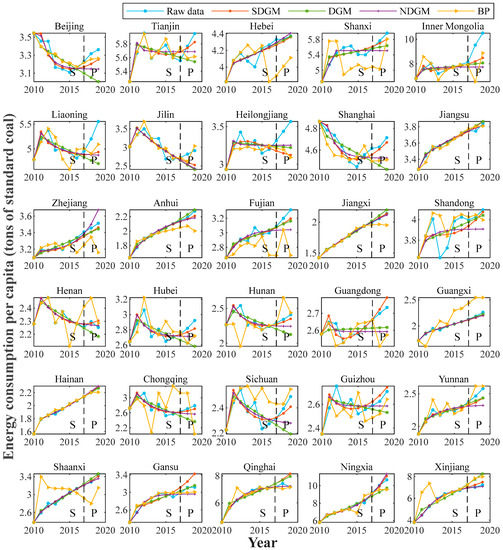
Figure 4.
Forecasted PCEC curves.
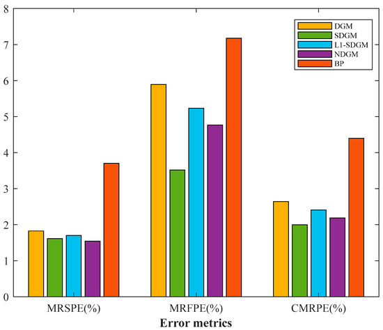
Figure 5.
Errors in the modeling results.
Table 4 lists the spatial correlation coefficients of the SDGM and L1-SDGM models, and the properties and characteristics of the spatial correlation effect of PCEC are analyzed. By comparing the spatial correlation coefficients of SDGM and L1-SDGM, we find that the coefficients for most regions are relatively similar, such as those for Beijing, Shanghai, and Anhui; however, there are still some regions with large differences in spatial correlation coefficients, such as Hebei, Liaoning, and Heilongjiang. This result indicates that there may be differences in the effects produced by spatial spillover in the lagged period and the current period and that each spatial unit is affected by its neighboring regions. The influence of the spatial spillover effect is time-varying. Based on the above comparison of the SDGM and L1-SDGM models, SDGM is more applicable in this example, so the spatial correlation coefficient of SDGM is analyzed here. Specifically, the spatial spillover of the PCECs of each province from 2010 to 2017 is comprehensively analyzed. First, the spatial correlation coefficients of three regions, Zhejiang, Hainan, and Ningxia, are negative, meaning that the growth of the PCECs of the adjacent provinces leads to a decline in the PCECs of these four regions to a certain extent. The spatial correlation coefficients of the PCECs of the other 27 regions are positive, which indicates that increases in the PCECs of the surrounding regions lead to increased PCECs for these four regions. Second, the spatial influence of the PCEC is most pronounced in Inner Mongolia, whereas Hainan is the least affected.
Table 4.
Spatial lag coefficients of PCECs for the SDGM and L1-SDGM models.
3.4. Projections of PCEC of China
Based on the model comparison above, SDGM is most applicable in this case; therefore, SDGM is selected to predict the PCECs of 30 provinces. Additionally, given the above analysis of the spatial correlation coefficients and the nature of the SDGM model, a metabolic concept is applied in forecasting [35,36]. The so-called metabolic concept involves reconstructing the model by eliminating irrelevant data from the original series based on the most recent data generated by the system, i.e., adding new data to the series while deleting the oldest available data so that the dimension of the data series remains fixed. In practical modeling, using the original data series for long-term prediction is not ideal in some cases because over time, the factors that influence the system change, and the state subsequently varies. When grey prediction models are built using original data, the reliability of predictions may decrease over time. Based on this metabolic approach, the most recent information is constantly added, thus gradually decreasing the grey level until the prediction objective is achieved.
We first use eight data points from 2012 to 2019 to predict 2020 data and then remove the old data from 2012, add the new predictions for 2020, and predict data for 2021. The final prediction results are presented in Figure 6 and Table 5, and the fitting errors are presented in Table 6. Notably, the fit of the SDGM model is good, with most error values below 1%. Good fitting accuracy is a prerequisite for an accurate prediction. In Figure 6, the forecasting results show that the PCECs of most Chinese provinces will increase in the future, which is consistent with the results of Lu et al. [59], whose projections indicate that the PCEC of China will continue to grow rapidly in the coming years; however, the PCEC of Tianjin will peak in 2024, the PCEC of Qinghai will remain largely unchanged, and the PCEC of Beijing will tend to decrease, possibly due to technological advances, a reduction in energy consumption in the surrounding areas, or supply-side reform to improve the efficiency of energy consumption in the Beijing–Tianjin region.
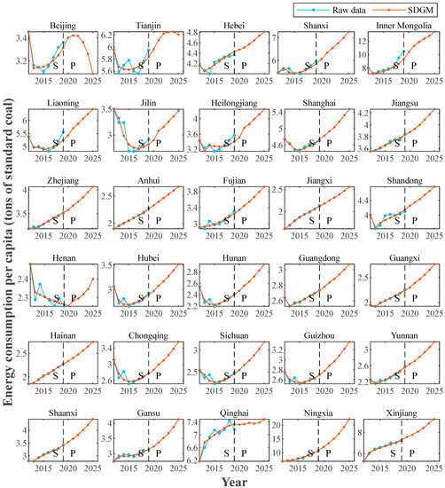
Figure 6.
Modeled prediction curves for the PCECs of the SDGM model.
Table 5.
PCEC prediction results (tons of standard coal).
Table 6.
Simulation error of the SDGM model.
4. Conclusions
This paper addresses the shortcomings of existing grey models relating to their abilities to model spatial variables. A spatial matrix is incorporated into DGM(1,1) on the basis of the advantages of the discrete grey model, which enhances spatial data prediction. Then, SDGM(1,1,m) with spatial characteristics, is established, and L1-SDGM(1,1,m) with spatial time lag effects is developed. The SDGM(1,1,m) and L1-SDGM(1,1,m) models are compared with the DGM(1,1), DGM(1,n), and BP neural network models using PCEC data from 30 Chinese provinces. The results verify the superiority of the SDGM(1,1,m) and L1- SDGM(1,1,m) models. SDGM(1,1,m) is also used to forecast the PCECs of 30 provinces in China. We draw the following conclusions. First, although SDGM(1,1,m) is similar to DGM(1,n), their modeling conditions, targets, and economic perspectives are obviously different. Second, compared with the DGM(1,1), DGM(1,n), NDGM(1,1)s and BP neural network models, the SDGM(1,1,m) and L1-SDGM(1,1,m) models provide enhanced forecasting performances by considering regional associations. Third, the SDGM(1,1,m) and L1-SDGM(1,1,m) models are more capable of capturing the most recent trends in the data than the DGM(1,1), NDGM(1,1), and BP neural network models are, and they better reflect the priority of new information. Fourth, the SDGM(1,1,m) and L1- SDGM(1,1,m) models can be used to effectively analyze the spatial correlations within the selected modeling interval and provide accurate predictions. Based on the spatial correlation coefficients of SDGM(1,1,m), the PCECs of Inner Mongolia and Qinghai are the most affected by spatial factors, and the PCECs of Jilin and Jiangxi are the least affected. Fifth, the predictions of SDGM(1,1,m) indicate that the PCECs of most regions of China will increase under the current grey conditions, while the PCEC in Beijing is expected to decline and the PCEC in Tianjin will peak in 2024.
In this paper, only the spatial matrix is incorporated into DGM(1,1), and whether the same optimization can be performed for other grey models is not discussed. Moreover, although the time lag effect of spatial spillover is considered, only the case with a one-period lag is modeled, and other cases are not discussed. In addition, only the PCEC is predicted, and the model’s application to other types of energy systems remains to be studied. The projections show that PCECs will tend to increase in most regions of China, but the reasons for this phenomenon are not revealed, nor are the problems or policy recommendations associated with the increase in energy consumption. All these limitations should be addressed in future research.
Author Contributions
Conceptualization, H.W. and Z.Z.; software Z.Z.; validation, H.W.; data curation, Z.Z.; writing—original draft, Z.Z.; writing—review and editing, H.W.; supervision, H.W. All authors have read and agreed to the published version of the manuscript.
Funding
This work was supported by the National Social Science Fund of China (No. 22XTJ004), the Social Science Project of Shaanxi (No. 2021D062), the National Statistical Science Research Project (No. 2022LY068), and the Humanities and Social Science Project of Chinese Ministry of Education (No. 22XJC790009).
Institutional Review Board Statement
Not applicable.
Informed Consent Statement
Not applicable.
Data Availability Statement
The datasets of this paper are available from the corresponding author on reasonable request.
Conflicts of Interest
The authors declare no conflict of interest.
References
- Barak, S.; Sadegh, S.S. Forecasting energy consumption using ensemble ARIMA–ANFIS hybrid algorithm. Int. J. Electr. Power 2016, 82, 92–104. [Google Scholar] [CrossRef]
- Cabral, J.dA.; Legey, L.F.L.; Freitas Cabral, M.V.d. Electricity consumption forecasting in Brazil: A spatial econometrics approach. Energy 2017, 126, 124–131. [Google Scholar] [CrossRef]
- Jamil, R. Hydroelectricity consumption forecast for Pakistan using ARIMA modeling and supply-demand analysis for the year 2030. Renew. Energy 2020, 154, 1–10. [Google Scholar] [CrossRef]
- Shahbaz, M.; Loganathan, N.; Sbia, R.; Afzad, T. The effect of urbanization, affluence and trade openness on energy consumption: A time series analysis in Malaysia. Renew. Sustain. Energy Rev. 2015, 47, 683–693. [Google Scholar] [CrossRef]
- Mirza, F.M.; Kanwal, A. Energy consumption, carbon emissions and economic growth in Pakistan: Dynamic causality analysis. Renew. Sustain. Energy Rev. 2017, 72, 1233–1240. [Google Scholar] [CrossRef]
- Xu, X.; Xiao, B.; Li, C.Z. Analysis of critical factors and their interactions influencing individual’s energy conservation behavior in the workplace: A case study in China. J. Clean. Prod. 2021, 286, 124955. [Google Scholar] [CrossRef]
- Oliveira, E.M.D.; Oliveira, F.L.C. Forecasting mid-long term electric energy consumption through bagging ARIMA and exponential smoothing methods. Energy 2018, 144, 776–788. [Google Scholar] [CrossRef]
- Tang, L.; Wang, X.F.; Wang, X.L.; Shao, C.C.; Liu, S.Y.; Tian, S.J. Long-term electricity consumption forecasting based on expert prediction and fuzzy Bayesian theory. Energy 2018, 167, 1144–1154. [Google Scholar] [CrossRef]
- Rodger, J.A. A fuzzy nearest neighbor neural network statistical model for predicting demand for natural gas and energy cost savings in public buildings. Expert Syst. Appl. 2014, 41, 1813–1829. [Google Scholar] [CrossRef]
- Ilbeigi, M.; Ghomeishi, M.; Dehghanbanadaki, A. Prediction and optimization of energy consumption in an office building using artificial neural network and a genetic algorithm. Sustain. Cities Soc. 2020, 61, 102325. [Google Scholar] [CrossRef]
- Papadimitriou, T.; Gogas, P.; Stathakis, E. Forecasting energy markets using support vector machines. Energy Econ. 2014, 44, 135–142. [Google Scholar] [CrossRef]
- Tziolis, G.; Spanias, C.; Theodoride, M.; Theocharides, S.; Lopez-Lorente, J.; Livera, A.; Makrides, G.; Georghiou, G.E. Short-term electric net load forecasting for solar-integrated distribution systems based on Bayesian neural networks and statistical post-processing. Energy 2023, 271, 127018. [Google Scholar] [CrossRef]
- Huang, L.Q.; Liao, Q.; Zhang, H.R.; Jiang, M.K.; Yan, J.; Liang, Y.T. Forecasting power consumption with an activation function combined grey model: A case study of China. Int. J. Electr. Power 2021, 130, 106977. [Google Scholar] [CrossRef]
- Xiao, Q.Z.; Shan, M.Y.; Gao, M.Y.; Xiao, X.P.; Goh, M. Parameter optimization for nonlinear grey Bernoulli model on biomass energy consumption prediction. Appl. Soft Comput. 2020, 95, 106538. [Google Scholar] [CrossRef]
- Xie, W.L.; Wu, W.Z.; Liu, C.; Zhao, J.J. Forecasting annual electricity consumption in China by employing a conformable fractional grey model in opposite direction. Energy 2020, 202, 11768. [Google Scholar] [CrossRef]
- Liu, C.; Wu, W.Z.; Xie, W.L.; Zhang, J. Application of a novel fractional grey prediction model with time power term to predict the electricity consumption of India and China. Chaos Solitons Fractals 2020, 141, 110429. [Google Scholar] [CrossRef]
- Şahin, U. Forecasting share of renewables in primary energy consumption and CO2 emissions of China and the United States under Covid-19 pandemic using a novel fractional nonlinear grey model. Expert Syst. Appl. 2022, 209, 118429. [Google Scholar] [CrossRef]
- Saxena, A. Optimized fractional overhead power term polynomial grey model (OFOPGM) for market clearing price prediction. Electr. Power Syst. Res. 2023, 214, 108800. [Google Scholar] [CrossRef]
- Deng, J. Control problems of grey systems. Syst. Control Lett. 1982, 5, 288–294. [Google Scholar]
- Ma, X.; Xie, M.; Wu, W.; Zeng, B.; Wang, Y.; Wu, X.X. The novel fractional discrete multivariate grey system model and its applications. Appl. Math. Model. 2019, 70, 402–424. [Google Scholar] [CrossRef]
- Xu, K.; Pang, X.Y.; Duan, H.M. An optimization grey Bernoulli model and its application in forecasting oil consumption. Math. Probl. Eng. 2021, 2021, 5598709. [Google Scholar] [CrossRef]
- Wu, L.F.; Liu, S.F.; Yao, L.G.; Yan, S.L.; Liu, D.L. Grey system model with the fractional order accumulation. Commun. Nonlinear Sci. Numer. Simul. 2013, 18, 1775–1785. [Google Scholar] [CrossRef]
- Xie, W.L.; Liu, C.; Wu, W.Z. The fractional non-equidistant grey opposite-direction model with time-varying characteristics. Soft Comput. 2020, 24, 6603–6612. [Google Scholar] [CrossRef]
- Liu, C.; Wu, W.Z.; Xie, W.L.; Zhang, T.; Zhang, J. Forecasting natural gas consumption of China by using a novel fractional grey model with time power term. Energy Rep. 2021, 7, 788–797. [Google Scholar] [CrossRef]
- Wu, L.F.; Liu, S.F.; Yang, Y.J. Using fractional order method to generalize strengthening generating operator buffer operator and weakening buffer operator. IEEE-CAA J. Autom. 2018, 5, 52–56. [Google Scholar]
- Zeng, B.; Duan, H.M.; Bai, Y.; Meng, W. Forecasting the output of shale gas in China using an unbiased grey model and weakening buffer operator. Energy 2018, 151, 238–249. [Google Scholar] [CrossRef]
- Wei, B.L.; Xie, N.M.; Hu, A.Q. Optimal solution for novel grey polynomial prediction model. Appl. Math. Model. 2018, 62, 717–727. [Google Scholar] [CrossRef]
- Ma, X.; Mei, X.; Wu, W.Q.; Wu, X.X.; Zeng, B. A novel fractional time delayed grey model with Grey Wolf Optimizer and its applications in forecasting the natural gas and coal consumption in Chongqing China. Energy 2019, 178, 487–507. [Google Scholar] [CrossRef]
- Şahin, U.; Şahin, T. Forecasting the cumulative number of confirmed cases of COVID-19 in Italy, UK and USA using fractional nonlinear grey Bernoulli model. Chaos Solitons Fractals 2020, 138, 109948. [Google Scholar] [CrossRef]
- Carmona-Benítez, R.B.; Nieto, M.R. SARIMA damp trend grey forecasting model for airline industry. J. Air Transp. Manag. 2020, 82, 101736. [Google Scholar] [CrossRef]
- Kang, Y.X.; Mao, S.H.; Zhang, Y.H. Variable order fractional grey model and its application. Appl. Math. Model. 2021, 97, 619–635. [Google Scholar]
- Xu, N.; Ding, S.; Gong, Y.D.; Bai, J. Forecasting Chinese greenhouse gas emissions from energy consumption using a novel grey rolling model. Energy 2019, 175, 218–227. [Google Scholar] [CrossRef]
- Ceylan, Z. Short-term prediction of COVID-19 spread using grey rolling model optimized by particle swarm optimization. Appl. Soft Comput. 2021, 109, 107592. [Google Scholar] [CrossRef] [PubMed]
- Zhou, W.H.; Zeng, B.; Wang, J.Z.; Luo, X.S.; Liu, X.Z. Forecasting Chinese carbon emissions using a novel grey rolling prediction model. Chaos Solitons Fractals 2021, 147, 110968. [Google Scholar] [CrossRef]
- Chen, K.; Laghrouche, S.; Djerdir, A. Degradation prediction of proton exchange membrane fuel cell based on grey neural network model and particle swarm optimization. Energy Convers. Manag. 2019, 195, 810–818. [Google Scholar] [CrossRef]
- Yang, X.Y.; Fang, Z.G.; Yang, Y.J.; Mba, D.; Li, X.C. A novel multi-information fusion grey model and its application in wear trend prediction of wind turbines. Appl. Math. Model. 2019, 71, 543–557. [Google Scholar] [CrossRef]
- Wang, Q.; Li, S.; Pisarenko, Z. Modeling carbon emission trajectory of China, US, and India. J. Clean. Prod. 2020, 258, 120723. [Google Scholar] [CrossRef]
- Xie, W.L.; Wu, W.Z.; Liu, C.; Zhang, T.; Dong, Z.J. Forecasting fuel combustion-related CO2 emissions by a novel continuous fractional nonlinear grey Bernoulli model with grey wolf optimizer. Environ. Sci. Pollut. Res. 2021, 28, 38128–38144. [Google Scholar] [CrossRef]
- Ye, L.L.; Xie, N.M.; Hu, A.Q. A novel time-delay multivariate grey model for impact analysis of CO2 emissions from China’s transportation sectors. Appl. Math. Model. 2021, 91, 493–507. [Google Scholar] [CrossRef]
- Rajesh, R. Predicting environmental sustainability performances of firms using trigonometric grey prediction model. Environ. Dev. 2023, 45, 100830. [Google Scholar] [CrossRef]
- Sapnken, F.E.; Tamba, J.G. Petroleum products consumption forecasting based on a new structural auto-adaptive intelligent grey prediction model. Expert Syst. Appl. 2022, 203, 117579. [Google Scholar] [CrossRef]
- Comert, G.; Khan, Z.; Rahman, M.; Chowdhury, M. Grey models for short-term queue length predictions for adaptive traffic signal control. Expert Syst. Appl. 2021, 185, 115618. [Google Scholar] [CrossRef]
- Saxena, A. Grey forecasting models based on internal optimization for Novel Coronavirus (COVID-19). Appl. Soft Comput. 2021, 111, 107735. [Google Scholar] [CrossRef] [PubMed]
- Xie, N.M.; Liu, S.F. Discrete grey forecasting model and its optimization. Appl. Math. Model. 2009, 33, 1173–1186. [Google Scholar] [CrossRef]
- Xie, N.M.; Liu, S.F.; Yang, Y.J.; Yuan, C.Q. On novel grey forecasting model based on non-homogeneous index sequence. Appl. Math. Model. 2013, 37, 5059–5068. [Google Scholar] [CrossRef]
- Ma, X.; Liu, Z.B. Research on the novel recursive discrete multivariate grey prediction model and its applications. Appl. Math. Model. 2016, 40, 4876–4890. [Google Scholar] [CrossRef]
- Jiang, S.Q.; Liu, S.F.; Liu, Z.X.; Fang, Z.G. Cubic time-varying parameters discrete grey forecasting model and its properties. Control Decis. 2016, 31, 279–286. [Google Scholar]
- Wei, B.L.; Xie, N.M.; Yang, Y.J. Data-based structure selection for unified discrete grey prediction model. Expert Syst. Appl. 2019, 136, 264–275. [Google Scholar] [CrossRef]
- Ding, S.; Li, R.J.; Tao, Z. A novel adaptive discrete grey model with time-varying parameters for long-term photovoltaic power generation forecasting. Energy Convers. Manag. 2021, 227, 113644. [Google Scholar] [CrossRef]
- Liu, C.; Xie, W.L.; Wu, W.Z.; Zhu, H.G. Predicting Chinese total retail sales of consumer goods by employing an extended discrete grey polynomial model. Eng. Appl. Artif. Intell. 2021, 102, 10426. [Google Scholar] [CrossRef]
- Gou, X.Y.; Zeng, B.; Gong, Y. Application of the novel four-parameter discrete optimized grey model to forecast the wastewater discharged in Chongqing China. Eng. Appl. Artif. Intell. 2022, 107, 104522. [Google Scholar] [CrossRef]
- Ye, L.; Yang, D.L.; Dang, Y.G.; Wang, J.J. An enhanced multivariable dynamic time-delay discrete grey forecasting model for predicting China’s carbon emissions. Energy 2022, 249, 123681. [Google Scholar] [CrossRef]
- Hao, Y.; Peng, H. On the convergence in China’s provincial per capita energy consumption: New evidence from a spatial econometric analysis. Energy Econ. 2017, 68, 31–43. [Google Scholar] [CrossRef]
- Hamilton, J.; Hogan, B.; Lucas, K.; Mayne, R. Conversations about conservation? Using social network analysis to understand energy practices. Energy Res. Soc. Sci. 2019, 49, 180–191. [Google Scholar] [CrossRef]
- Radmehr, R.; Henneberry, S.R.; Shayanmehr, S. Renewable energy consumption, CO2 emissions, and economic growth nexus: A simultaneity spatial modeling analysis of EU countries. Struct. Chang. Econ. Dyn. 2021, 57, 13–27. [Google Scholar] [CrossRef]
- Bu, Y.; Wang, E.; Bai, J.; Shi, Q. Spatial pattern and driving factors for interprovincial natural gas consumption in China: Based on SNA and LMDI. J. Clean. Prod. 2020, 263, 121392. [Google Scholar] [CrossRef]
- Elhorst, J.P. Matlab software for spatial panels. Int. Reg. Sci. Rev. 2014, 37, 389–405. [Google Scholar] [CrossRef]
- Wang, H.P.; Zhang, Z. Forecasting Chinese provincial carbon emissions using a novel grey prediction model considering spatial correlation. Expert Syst. Appl. 2022, 209, 118261. [Google Scholar] [CrossRef]
- Lu, Y.; Liu, C.; Pang, H.; Feng, T.; Dong, Z. Forecasting China’s per capita living energy consumption by employing a novel DGM (1, 1, tα) model with fractional order accumulation. Math. Probl. Eng. 2021, 2021, 6635462. [Google Scholar] [CrossRef]
Disclaimer/Publisher’s Note: The statements, opinions and data contained in all publications are solely those of the individual author(s) and contributor(s) and not of MDPI and/or the editor(s). MDPI and/or the editor(s) disclaim responsibility for any injury to people or property resulting from any ideas, methods, instructions or products referred to in the content. |
© 2023 by the authors. Licensee MDPI, Basel, Switzerland. This article is an open access article distributed under the terms and conditions of the Creative Commons Attribution (CC BY) license (https://creativecommons.org/licenses/by/4.0/).