Abstract
This study presents a novel approach to a mixed-integer linear programming (MILP) model for periodic inventory management that combines reinforcement learning algorithms. The rolling horizon method (RHM) is a multi-period optimization approach that is applied to handle new information in updated markets. The RHM faces a limitation in easily determining a prediction horizon; to overcome this, a dynamic RHM is developed in which RL algorithms optimize the prediction horizon of the RHM. The state vector consisted of the order-up-to-level, real demand, total cost, holding cost, and backorder cost, whereas the action included the prediction horizon and forecasting demand for the next time step. The performance of the proposed model was validated through two experiments conducted in cases with stable and uncertain demand patterns. The results showed the effectiveness of the proposed approach in inventory management, particularly when the proximal policy optimization (PPO) algorithm was used for training compared with other reinforcement learning algorithms. This study signifies important advancements in both the theoretical and practical aspects of multi-item inventory management.
1. Introduction
In recent years, companies have increasingly adopted artificial intelligence (AI) to optimize operations, resource allocation, and decision making. Reinforcement learning (RL), a subfield of AI, has emerged as a critical research area because of its extensive impact on various industry domains such as supply chain management, production, logistics, quality control, and inventory management. In the realm of inventory management, effective multi-item inventory management is crucial in maintaining optimal stock levels, reducing costs, and effectively responding to dynamic market situations through efficient replenishment planning.
In real-world cases, Samsung implemented an AI-based inventory management system that uses machine learning algorithms to predict demand and optimize inventories [1]. Amazon also utilizes machine-learning-based demand forecasting, which combines historical data, real-time data, and external factors such as weather [2]. Alibaba has also applied AI-based demand forecasting to its online marketplace [3]. Global companies are continually developing multi-item replenishment strategies to optimize their inventory in response to diverse consumer needs.
Although some researchers have explored the application of RL to aspects of inventory management such as demand forecasting, order quantity optimization, and reorder point determination, research on RL-based replenishment strategies is still in its infancy [4]. Most studies on multi-item replenishment strategies have traditionally focused on determining the optimal order period (joint replenishment problem) or order quantity (can-order policy, COP) using operational research techniques, often struggling to manage conditions characterizing the dynamic nature of real-world environments, such as unpredictable market demands. They are deterministic and incapable of incorporating real-time market information updates during model execution. To overcome this limitation, the rolling horizon method (RHM), which provides a mechanism for iteratively incorporating updated information into the decision-making process, is applied. However, the RHM struggles with easily setting the optimal prediction horizon, significantly affecting the efficiency of replenishment decisions. To address this issue, this study incorporated RL into RHM to dynamically optimize the prediction horizon, thereby enhancing the efficiency and effectiveness of the multi-item replenishment strategy. In the semiconductor manufacturing industry, the chips are produced by processing silicon wafers at a fabrication/test node, assembling die and packages at an assembly/test node, and finalizing the product before it is shipped to fulfill customer orders. In such circumstances, the supply chain experiences significant variations in processing time, yield, and demand uncertainty, necessitating the optimization of the prediction horizon tailored to the situation [5,6]. Thus, this innovative combination of the RHM and RL creates a pathway for a more responsive and adaptive inventory management system.
This study proposes a MILP model for a periodic COP, which is a widely used multi-item replenishment strategy that accounts for the correlation between multiple items and their integrated replenishment at regular intervals. The study also puts forward an RHM for updating the actual demand for items in the planning horizon and managing the replenishment schedules for future periods. Furthermore, this study introduces a dynamic RHM with RL that sets the MILP model of a periodic COP as the environment and the interval length of the RHM as the action space. Our research has two primary contributions. First, it aims to offer a flexible and adaptive decision-making framework that addresses the challenges of scalability and responsiveness to dynamic environments in real-world inventory management. Second, by integrating the strengths of these techniques, this study seeks to provide a scalable and adaptive solution to the inventory management challenges faced by companies.
The remainder of this paper is organized as follows. Section 2 presents the literature review. Section 3 introduces the assumptions, problem definitions, and optimization models. Section 4 describes the development of the RHM and dynamic RHM using RL. Section 5 presents the verification of the efficiency of the proposed optimization model and algorithms through various numerical experiments. Section 6 presents academic and managerial insights regarding the research. Finally, Section 7 summarizes the research and concludes the paper.
2. Literature Review
This study focuses on three research areas of inventory management: COP, RHM, and RL. Regarding COP, it is an inventory management approach that focuses on ordering items in multi-item systems; researchers have explored this approach in different contexts. Kayiş, Bilgiç, and Karabulut [7] examined a two-item continuous-review inventory system with independent Poisson demand processes and economies of scale in joint replenishment and proposed and modeled a COP as a semi-Markov decision process using a straightforward enumeration algorithm. Nagasawa et al. [8] suggested a method for determining the optimal parameter of a periodic COP for each item in a lost sales model using a genetic algorithm. The primary goal was to minimize the number of orders, inventory, and shortages compared to those in a conventional joint replenishment problem. Noh, Kim, and Hwang [9] explored multi-item inventory management with carbon cap-and-trade under limited storage capacity and budget constraints. The periodic coefficient of performance was used to address this issue. However, previous studies have limitations in handling demand and supply uncertainties and lack robust methods for optimizing replenishments and minimizing costs.
The RHM is a planning and decision-making technique that involves breaking down a long-term planning horizon into smaller overlapping sub-horizons. Many researchers have employed the RHM to overcome the limitations of deterministic environments. Tresoldi and Ceselli [10] suggested a practical optimization approach based on the RHM to address general single-product periodic-review inventory control challenges. Al-Ameri, Shah, and Papageorgiou [11] aimed to develop a dynamic vendor-managed inventory (VMI) system and proposed various optimization algorithms to solve the problem using the RHM. The VMI system was modeled as a MILP model using a discrete-time representation with a mathematical representation following the resource-task network formulation. Xie, Wang, and Yang [12] investigated an infinite-horizon stochastic inventory system with multiple supply sources and proposed a robust RHM. Noh and Hwang [13] created an optimization model using MILP to address energy supply chain management (ESCM) problems involving supplier selection in emergency procurement scenarios; the model considered a single thermal power plant and multiple fossil fuel suppliers. To effectively manage uncertainties, they employed an RHM capable of handling the ESCM under uncertain conditions. As previous studies have shown, the RHM is widely used to solve issues related to uncertainties and introduce dynamism to the MILP model.
Researchers have explored the application of RL in inventory management and used training agents to make optimal ordering decisions through environmental interactions, enabling inventory strategies to adapt dynamically to demand and supply uncertainties. Kara and Dogan [14] studied two distinct ordering policies using RL and highlighted the significance of age information in perishable inventory systems. The problem was modeled using RL and optimized using Q-learning and SARAS (state–action–reward–state–action) learning. Chen et al. [15] proposed a blockchain-based framework for agri-food supply chains, offering product traceability and an RL-based supply chain management method for making effective production and storage decisions for agri-food products and thereby optimizing profits. The findings demonstrated that the RL-based supply chain management method outperformed heuristic and Q-learning approaches in terms of product profits. Chong, Kim, and Hong [16] presented a deep reinforcement learning method for optimizing apparel supply chains, focusing on the soft actor–critic (SAC) model. A comparison of the six RL models revealed that the SAC model effectively balanced the service level and sell-through rate while minimizing the inventory-to-sales ratio. Meisheri et al. [17] tackled the challenges of multi-product, multi-period inventory management using deep RL. Their approach improved inventory control in several ways: the simultaneous management of multiple products under realistic constraints, the need for minimal retraining requirements for the RL agent when system changes occur, and the efficient handling of multi-period constraints arising from varying lead times for different products. Boute et al. [4] discussed the critical design aspects of deep RL algorithms for inventory control, addressing implementation challenges and associated computational efforts. Many researchers have applied RL to inventory management research; however, its application in this research is mostly limited to determining the number of orders or production items. Departing from the application of RL in previous studies, this study applies RL to improve the scheduling of the RHM, overcoming the limitation of the MILP model.
3. Optimization Model
All the notations associated with the optimization model are presented in Appendix A.
3.1. Assumptions and Problem Definition
There are five assumptions in this study.
- The system considers a periodic review COP in which a single buyer orders multiple items;
- When the inventory level of an item drops below the reorder point, that item is replenished along with any other item whose inventory level is below the can-order level. Both the reorder point and COP are assumed to be constant;
- The procurement lead time of each item is a multiple of the inventory review period of a buyer;
- There is a correlation between the items considered in the study;
- The demand for each item follows a specific probability distribution.
Problem Definition
This problem addresses a periodic COP that minimizes the total cost of a buyer when the demand for an item follows a specific probability distribution and the supplier has a procurement lead time. Specifically, the order placement follows a designated timeline. Relying solely on reorder points for procurement decisions might expose the buyer to a high risk of stock-outs until the subsequent order cycle. By implementing the periodic COP, the buyer can leverage the can-order level to proactively replenish potentially out-of-stock items, thus ensuring a sustained service level. Thus, the buyer periodically checks inventory levels and determines the optimal order quantities of items based on pre-established reorder points and the can-order level. Then, the buyer places an order that considers the lead time for each item. The orders are replenished sequentially over time as the planning horizon unfolds. The replenished items need to arrive within the planning horizon, and the last ordering time of the buyer for each item, excluding the item-specific lead time, is .
3.2. Mathematical Model
In this section, the establishment of the MILP model for the periodic COP with procurement lead time is described. The total cost of a buyer during the planning horizon consists of the ordering, backordering, and holding costs. The ordering cost is determined by the replenishment decision of a buyer at time , and the ordering cost for planning horizon can be expressed as shown in Equation (1):
The planning horizon of a buyer is fixed, and their actual ordering period, excluding the procurement lead time for each item, is . For example, if the planning horizon is four weeks, and the procurement lead time for item is one week, the last time to place an order for item is at the end of week three. Item is replenished in the last planning horizon, i.e., week 4. If the buyer orders an item in week 4, it will be replenished in week 5; this replenishment is unintended, as it goes beyond the planning horizon. In Equation (1), is a binary variable that determines the replenishment decision. If the buyer orders one of the items, becomes one, and an ordering cost is incurred. If the buyer does not order any items, is zero, and no ordering cost is incurred.
The holding cost of item at time is calculated based on the average inventory level at time . This level is the mean of the order-up-to level at the beginning of time and the inventory level at the end of time . Equation (2) shows the holding costs for all the items during the planning horizon:
Equation (3) represents the backorder cost of item during the planning horizon :
The total cost of a buyer is the sum of the order, holding, and backorder costs during the planning period; this cost is mathematically represented in Equation (4):
Following this mathematical model, the MILP model was developed.
Equation (5) shows that the net inventory level of the item expected at the end of the planning period can be expressed as the sum of the previous order quantity and the initial inventory level at the beginning of the period. Equation (6) represents the expected net inventory level at the end of the period, with Equation (7) guaranteeing that the inventory level is equal to the difference between the on-hand inventory and backorder levels. Equation (8) represents the major ordering cost incurred when at least one item is ordered, while Equations (9) and (10) represent the regulated ordering that occurs when the inventory position falls below the reordering point. According to Equations (11) and (12), if the inventory position at the end of the previous period is below the reorder point, the item is ordered in an amount equal to the difference between the order-up-to level and the inventory level at the end of the previous period. Equations (13) and (14) can determine whether the inventory level is below the can-order level. According to Equations (15)–(19), if the inventory level of at least one item is below its reorder point, the following order includes other items whose inventory levels are below their can-order levels. According to Equations (20) and (21), if the inventory level at the end of the previous period is below the can-order level, that item is ordered in an amount equal to the difference between its order-up-to level and the inventory level at the end of the previous period. Equation (22) represents the regulation of the ordering of items whose inventory levels are below the reorder or can-order levels. Equations (23) and (24) indicate that the order-up-to-level is set based on the inventory level, which is below the reorder point or can-order level.
4. Algorithms
4.1. Rolling Horizon Method
The RHM is a well-known approach in operations research, particularly in planning and scheduling problems, where the objective is to make a series of decisions over time. By breaking down the decision-making process into smaller overlapping subproblems, the RHM enables the incorporation of updated information into mathematical programming models and facilitates adaptation to changing conditions. The RHM consists of several key components, including the control horizon, prediction horizon, planning horizon, and time step. The prediction horizon refers to the interval length in which a model forecasts demand or optimizes planning and scheduling. The planning horizon is the total time over which a model optimizes its decisions, and the update frequency determines how often a model is updated with new information. The RHM offers several advantages in the context of inventory management, such as increased flexibility and adaptability to changing market conditions. Furthermore, it can handle the deterministic problem of a MILP model. Figure 1 shows the concept of the RHM.
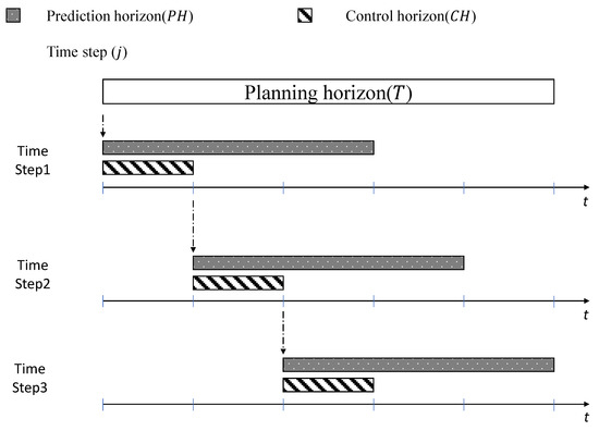
Figure 1.
Concept of the RHM.
RHM
Step 1. Set input parameter
- Set planning horizon, control horizon, and prediction horizon.
Step 2. Solve MILP
- Order products based on the result of the optimal solution.
Step 3. Update information
- Check inventory level based on real demand during the control horizon.
Step 4. Check iteration condition
- Repeat Step 2 and Step 3 at the end of the planning horizon.
Step 5. End RHM
4.2. Dynamic Rolling Horizon Method
This subsection discusses the proposed dynamic RHM based on state-of-the-art RL algorithms and proximal policy optimization (PPO), which is a model-free on-policy algorithm and a well-known policy gradient method. The PPO algorithm primarily differs from other RL algorithms in that it optimizes a surrogate objective function to prevent excessively large policy updates. The policy gradient loss function for a single trajectory in the vanilla policy gradient method is expressed as follows:
where is the policy (with representing the policy parameters), is the action at timestep , is the state at timestep . is the expected return (cumulative future reward) function. The PPO algorithm modifies the policy gradient loss function to constrain the policy updates, ensuring that the new policy does not deviate too much from the old policy . The loss function in PPO is as follows:
where is the probability ratio, and is a hyperparameter that determines the degree of the policy update. The clip function ensures that is in the range . is the advantage function at timestep . Therefore, the loss function encourages policy updates to be small. Regarding , it is maximized using stochastic gradient ascent, with multiple epochs over the mini-batches of the collected trajectories. The PPO algorithm repeatedly performs this process by collecting new trajectories using the latest policy after each update.
Owing to the characteristics of the MILP model, demand information cannot be updated in real time. To handle demand uncertainties, buyers predict future demand and order items at the beginning of each period while simultaneously proposing future replenishment quantities to suppliers, allowing both buyers and suppliers to prepare for future uncertainties. A dynamic RHM with RL is a solution in which RH is applied to RHM. Regarding the application of RL, the MILP model of the periodic COP and the interval length of the RHM were set as the environment and action space, respectively. Figure 2 shows the framework of the dynamic RHM.
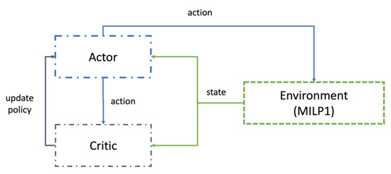
Figure 2.
Framework of the dynamic RHM.
The state in time step includes the beginning and end of the control horizon during the RHM progress. First, it involves the order-up-to-level of each item at the beginning of the control period. Second, it involves the system information that is confirmed and updated at the end of the control horizon after the calculation of the MILP model, which includes the real demand, total cost (), holding cost (, and backorder cost () at the current time step. The equations related to the actual cost incurred at time step are as follows:
Additionally, when the control horizon ends, the difference between the order-up-to level of each item and the actual demand is added to the order quantity determined from the MILP model calculation in the previous time step. This calculation becomes ordered up to the level for the next time step. Equations (30)–(32), which are based on Equations (5) and (6), reflect the replenishment of the order quantity decided through the MILP model in the previous time step. The state defined in this study is shown in Equation (33). The state space of both the order-up-to level and actual demand increases in accordance with the number of items.
The action state in time step includes the prediction horizon of the RHM, the interval length in the MILP model, and the forecasting demand. The upper limit of the prediction horizon is determined based on the planning horizon set by the decision-maker. For instance, if the decision-maker replenishes once a week and requires a two-month schedule plan, the upper limit of the prediction horizon is eight weeks. The lower limit of the prediction horizon is the sum of the control horizon and the longest lead time among the items. If the control horizon is one week, and the longest lead time for an item is two weeks, the prediction horizon, including the control period and lead time, is three weeks. Therefore, in the aforementioned scenario, the total number of possible actions (or prediction horizons) ranged from three to eight weeks. In dynamic RHM, both the prediction and planning horizons are determined as positive multiples of the control horizon.
Rewards are a critical factor influencing the learning performance of RL. The dynamic RHM employs a reward function that compares the total cost of the previous and current time steps using Equation (30). Equation (35) represents the reward function used in this study:
5. Numerical Experiments
Two types of numerical experiments were conducted to verify the dynamic RHM performance. The first experiment was a comparison test among the RL algorithms advantage actor–critic (A2C), asynchronous advantage actor–critic (A3C), and PPO. Those algorithms are famous model-free on-policy algorithms and can handle both discrete and continuous actions. In the action space, the prediction horizon is set as discrete actions and forecasting demand is set as continuous actions. In the second experiment, an efficiency improvement experiment was conducted under an uncertain demand pattern. The models were trained for 5000 episodes (epochs), with each episode lasting 52 weeks. The buyer considered three types of items. The reorder point and the can-order level for the items were set as and , respectively, and big-M was set to 100,000. According to Equation (35), if the total cost of each time step is less than the total cost of the previous time step, the buyer will have an appropriate order quantity and inventory level in response to the demand. Table 1 lists the hyperparameters used in RL training. The proposed model and algorithm were coded using PyTorch 2.0, Gymnasium 0.28, and Ray 2.4.0. The MILP model was solved using the GUROBI Optimizer 10.0.0. Both observation normalization and reward normalization were used to create a stable learning environment. The numerical experiments were performed on a computer with Ryzen 5950x at 3.4 GHz, 128 GB RAM, and GeForce RTX 3090.

Table 1.
Hyperparameters in RL training.
5.1. Experiment Reflecting Situation with Demand Following a Specific Probability Distribution
In this experiment, only the interval length was set as the action of the agent. In this case, a stable situation, in which the demand for the item followed a specific probability distribution and fluctuated less, was considered. Thus, the action space was set as . The input parameters for each item are listed in Table 2, which shows that the out-of-stock costs are higher than the storage costs. It was assumed that the demand followed a normal distribution, and the forecasted demand was assumed to be the mean of the normal distribution. An evaluation reward was used to evaluate the algorithms. The model received a reward during the evaluation process, which was calculated after the epoch; this reward measured the degree to which the model generalized the new data.
Table 2.
Input parameters in the first experiment.
Figure 3 shows the mean evaluation rewards for the dynamic RHM using the RL algorithms. Although training continued, the evaluation rewards of the three algorithms did not converge and were amplified within the same range, implying that the RL algorithms had not been trained. The dynamic RHM sets both the order up-to-level and actual demand as the state. Since the predicted demand was fixed as the average of the normal distribution, the interval length, which was the action of the agent, did not significantly affect performance improvement.
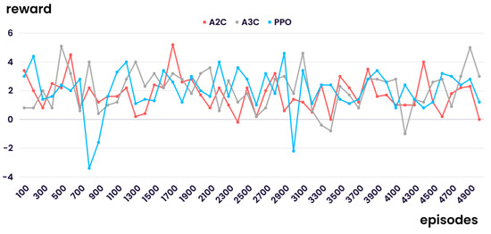
Figure 3.
Results of the first experiment.
5.2. Experiment Reflecting Situation with Demand Implying Uncertainty
This experiment aimed to confirm the efficiency of the dynamic RHM under an uncertain demand pattern where the demand for the items did not follow a specific probability distribution. Figure 4 shows the demand patterns for these items. Equation (33) was used to represent the action space in this experiment. At each time step, the agent determines the forecast demand for the next time step as an action.
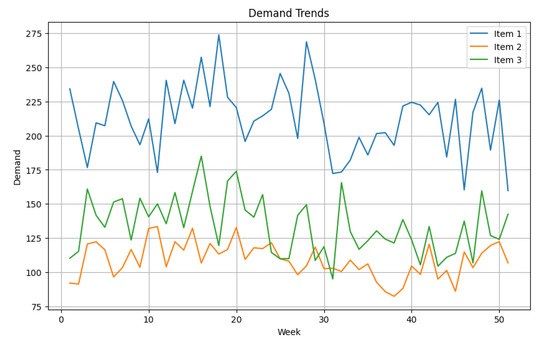
Figure 4.
Demand patterns for three items.
As shown in Figure 5, the evaluation reward converged as the number of training episodes increased. Comparing the three types of RL algorithms, the state-of-the-art RL algorithm PPO exhibited the best performance in terms of evaluation rewards, while A2C and A3C were similar in terms of these rewards. At the beginning of the training, the evaluation rewards of the three algorithms did not differ significantly; however, the performance of PPO improved as learning progressed. In A2C and A3C, the evaluation reward did not improve significantly after approximately 1300 episodes, indicating that long-term learning was not significant. In contrast, PPO only converged after learning approximately 2000 times or more. However, in this experiment, the time required by PPO to learn episodes was disadvantageously approximately twice as long as that required by A2C and AC3; PPO produced better results with less learning (episodes of less than 1000). Thus, the dynamic RHM with PPO was more efficient compared to the dynamic RHM with the other two algorithms.
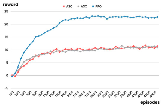
Figure 5.
Results of the second experiment.
Figure 6 shows the comparison of computing time among AC2, AC3, and PPO. A3C, with its asynchronous update feature, exhibits the fastest training times across different training scales, from 1000 to 5000 training. PPO, though more computationally demanding per update and exhibiting the longest training times in this comparison, is more practical due to its stability and efficiency. This result presents the importance of choosing the appropriate algorithm based on the specific requirements of computational resources, the problem complexity, and the desired balance between speed and stability.
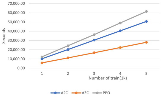
Figure 6.
Comparison of computing time.
5.3. Comparision Experiment of Dynamic RHM Regarding Interval Length
In this experiment, I evaluate the performance of three RL algorithms post 5000 episodes of training. The test is conducted over a planning horizon of 10 weeks. Table 3 presents the results of this experiment, showing interval lengths proposed by each of the three algorithms. Consistent with the outcomes depicted in Figure 5, PPO demonstrates the most efficient performance, as indicated by the lowest total cost. In contrast, A2C exhibits a relatively higher total cost.
Table 3.
Results of comparison experiments regarding interval length.
Analyzing the results in conjunction with those from Section 5.2, it appears that A3C can apply effective learning within a shorter time. However, it is crucial to note that the performance of RL algorithms can be highly dependent on the specific problem and the hyperparameters used. Furthermore, due to the stochastic nature of RL, the results could vary if the experiment were to be repeated.
6. Insights
6.1. Academic Insights
This study contributes to the existing literature on RL-based inventory management by proposing a MILP model for periodic COP and integrating it with RL algorithms. The RHM has been widely used to solve MILP problems; however, determining the optimal prediction horizon can be difficult. Many studies have used the prediction horizon as a sensitivity analysis tool or relied on the choice of the decision-maker. This study presents a new direction for RL research. The dynamic RHM presented in this study uses RL to improve the response of the existing RHM to market conditions. The proposed algorithm addresses the dynamic nature of multi-item inventory management and provides a flexible framework for updating demand information at planning intervals. The traditional mathematical programming approach with the latest RL algorithms is presented as a new research direction for multi-item inventory management.
6.2. Managerial Insights
The proposed algorithm provides an adaptive solution for companies (buyers) to manage the market and their associated suppliers under uncertain conditions. Using this method, the buyer can simultaneously determine the optimal order quantity while setting the optimal schedule (prediction horizon) according to market changes. In particular, the ordering period is a specific period. If a buyer orders an item using only the reorder point, there is a high probability that the item will be out of stock until the next order period. Using this periodic COP model, buyers can use the can-order level to order items that may soon be out of stock and thereby maintain a stable service level. Therefore, through the contributions of this study, decision-makers can improve the overall efficiency of inventory management systems.
7. Conclusions
In this paper, a MILP model for periodic COP, a well-known multi-item replenishment policy, is developed. Also, a dynamic RHM to optimize the prediction horizon using RL algorithms is introduced. To reflect practical scenarios, we considered the lead time until the buyer ordered and received a product. The RHM was applied to enable the demand for a product to follow a normal distribution or respond to uncertain situations. The RHM has traditionally been widely used to solve the deterministic problem of MILP; however, determining the appropriate prediction horizon can be challenging. Therefore, this study presents a dynamic RHM in which RL algorithms are used to determine its prediction horizon.
The proposed MILP model was selected as the environment for the dynamic RHM. The state vector consisted of the up-to-level order, real demand, total, holding, and backorder costs. The action vector was the prediction horizon of the RHM and forecasting demand for the next time step. The reward was defined as the difference between the total cost of the previous and current time steps. Thus, if the total cost of each time step was less than the total cost of the previous time step, the buyer would have an appropriate order quantity and inventory level in response to the demand. Three model-free-policy RL algorithms, namely A2C, A3C, and PPO, were used to build the dynamic RHM.
Three experiments were conducted to determine the efficiency of the proposed MILP model and algorithm. The first experiment considered a situation in which the demand was stable and normally distributed. Here, the action vector comprised only the prediction horizon, but learning did not converge even after 5000 epochs. In the second experiment, a situation in which the demand was uncertain was considered, and the original action vector was used. The results revealed that all three RL algorithms had been well-trained. The PPO algorithm performed the best among the three algorithms, even with a small number of epochs. However, A3C completed the learning faster than the other two algorithms. The third experiment compares the three RL algorithms regarding interval lengths. Again, PPO obtains the lowest total cost among the three algorithms.
This study presents an innovative intersection of RL with a traditional mathematical programming model for multi-item inventory management. It extends the RHM and offers a dynamic solution to overcome the weaknesses of the MILP model. In practice, the proposed adaptive algorithm boosts inventory management efficiency by preventing stock-outs and improving decision making under uncertain market conditions, representing a significant advancement in both academic and practical realms. However, there are also some limitations to be addressed. First, only three RL algorithms (A2C, A3C, and PPO) were considered for comparison. Other RL algorithms and variations may yield different results and potentially provide better results. Second, this study only considered the periodic COP. The proposed model did not account for factors such as multi-echelon supply chains, capacity constraints, the perishability of items, and supply chain disruptions. There are opportunities for future research to respond to these limitations. First, other RL algorithms, such as Deep Q Networks, can be considered. Second, the dynamic RHM framework can be extended to handle more complex real-world scenarios, such as those involving multi-echelon supply chains, the inventory management of perishable items, or supply chain disruptions.
Funding
This work was supported by the research fund of Hanyang University (HY-2023-1795).
Institutional Review Board Statement
Not applicable.
Informed Consent Statement
Not applicable.
Data Availability Statement
The data will be made available on request from the corresponding author.
Conflicts of Interest
The author declares no conflict of interest.
Nomenclature
| AI | Artificial Intelligence |
| COP | Can-order Policy |
| MILP | Mixed-integer linear programming |
| RHM | Rolling horizon method |
| RL | Reinforcement learning |
| A2C | Advantage actor–critic |
| A3C | Asynchronous advantage actor–critic |
| PPO | Proximal policy optimization |
| DQN | Deep-Q network |
Appendix A. Notations
| Index | |
| item, | |
| period, | |
| timestep, | |
| Decision variables | |
| Binary variable when an order is confirmed during period | |
| Order-up-to-level of item at period | |
| If drops below , then ; otherwise, | |
| If drops below , then ; otherwise, | |
| If drops below , and at least one item is ordered in period , then ; otherwise, | |
| Prediction horizon at timestep | |
| Variables | |
| Inventory level of item at the end of period | |
| On-hand inventory level of item at the end of period | |
| Backorder inventory level of item at the end of period | |
| Order quantity of item at period | |
| Number of items ordered at period | |
| Parameters of the policy | |
| Hyperparameter in PPO controls the degree of policy update | |
| Parameters | |
| Ordering cost at period | |
| Backorder cost of item at period | |
| Holding cost of item at period | |
| Initial inventory level of item | |
| Replenishment quantity of item , which is ordered before the planning horizon, at period | |
| Forecasted demand of item during period | |
| Real demand of item during period | |
| Can-order level of item | |
| Reorder point of item | |
| Lead time of item | |
| Large number | |
References
- Marilú Destino, J.F.; Müllerklein, D.; Trautwein, V. To Improve Your Supply Chain, Modernize Your Supply-Chain IT. 2022. Available online: https://www.mckinsey.com/capabilities/operations/our-insights/to-improve-your-supply-chain-modernize-your-supply-chain-it (accessed on 12 May 2023).
- AmazonWebServices. Predicting The Future of Demand: How Amazon Is Reinventing Forecasting with Machine Learning. 2021. Available online: https://www.forbes.com/sites/amazonwebservices/2021/12/03/predicting-the-future-of-demand-how-amazon-is-reinventing-forecasting-with-machine-learning/ (accessed on 12 May 2023).
- Mediavilla, M.A.; Dietrich, F.; Palm, D. Review and analysis of artificial intelligence methods for demand forecasting in supply chain management. Procedia CIRP 2022, 107, 1126–1131. [Google Scholar] [CrossRef]
- Boute, R.N.; Gijsbrechts, J.; Van Jaarsveld, W.; Vanvuchelen, N. Deep reinforcement learning for inventory control: A roadmap. Eur. J. Oper. Res. 2022, 298, 401–412. [Google Scholar] [CrossRef]
- Kempf, K.G. Control-oriented approaches to supply chain management in semiconductor manufacturing. In Proceedings of the 2004 American Control Conference, Boston, MA, USA, 30 June–2 July 2004; pp. 4563–4576. [Google Scholar]
- Schwartz, J.D.; Wang, W.; Rivera, D.E. Simulation-based optimization of process control policies for inventory management in supply chains. Automatica 2006, 42, 1311–1320. [Google Scholar] [CrossRef]
- Kayiş, E.; Bilgiç, T.; Karabulut, D. A note on the can-order policy for the two-item stochastic joint-replenishment problem. IIE Trans. 2008, 40, 84–92. [Google Scholar] [CrossRef]
- Nagasawa, K.; Irohara, T.; Matoba, Y.; Liu, S. Applying genetic algorithm for can-order policies in the joint replenishment problem. Ind. Eng. Manag. Syst. 2015, 14, 1–10. [Google Scholar] [CrossRef]
- Noh, J.; Kim, J.S.; Hwang, S.-J. A Multi-Item Replenishment Problem with Carbon Cap-and-Trade under Uncertainty. Sustainability 2020, 12, 4877. [Google Scholar] [CrossRef]
- Tresoldi, E.; Ceselli, A. Rolling-Horizon Heuristics for Capacitated Stochastic Inventory Problems with Forecast Updates. In Advances in Optimization and Decision Science for Society, Services and Enterprises; ODS: Genoa, Italy, 2019; pp. 139–149. [Google Scholar]
- Al-Ameri, T.A.; Shah, N.; Papageorgiou, L.G. Optimization of vendor-managed inventory systems in a rolling horizon framework. Comput. Ind. Eng. 2008, 54, 1019–1047. [Google Scholar] [CrossRef]
- Xie, C.; Wang, L.; Yang, C. Robust inventory management with multiple supply sources. Eur. J. Oper. Res. 2021, 295, 463–474. [Google Scholar] [CrossRef]
- Noh, J.; Hwang, S.-J. Optimization Model for the Energy Supply Chain Management Problem of Supplier Selection in Emergency Procurement. Systems 2023, 11, 48. [Google Scholar] [CrossRef]
- Kara, A.; Dogan, I. Reinforcement learning approaches for specifying ordering policies of perishable inventory systems. Expert Syst. Appl. 2018, 91, 150–158. [Google Scholar] [CrossRef]
- Chen, H.; Chen, Z.; Lin, F.; Zhuang, P. Effective management for blockchain-based agri-food supply chains using deep reinforcement learning. IEEE Access 2021, 9, 36008–36018. [Google Scholar] [CrossRef]
- Chong, J.W.; Kim, W.; Hong, J.S. Optimization of Apparel Supply Chain Using Deep Reinforcement Learning. IEEE Access 2022, 10, 100367–100375. [Google Scholar] [CrossRef]
- Meisheri, H.; Sultana, N.N.; Baranwal, M.; Baniwal, V.; Nath, S.; Verma, S.; Ravindran, B.; Khadilkar, H. Scalable multi-product inventory control with lead time constraints using reinforcement learning. Neural Comput. Appl. 2022, 34, 1735–1757. [Google Scholar] [CrossRef]
Disclaimer/Publisher’s Note: The statements, opinions and data contained in all publications are solely those of the individual author(s) and contributor(s) and not of MDPI and/or the editor(s). MDPI and/or the editor(s) disclaim responsibility for any injury to people or property resulting from any ideas, methods, instructions or products referred to in the content. |
© 2023 by the author. Licensee MDPI, Basel, Switzerland. This article is an open access article distributed under the terms and conditions of the Creative Commons Attribution (CC BY) license (https://creativecommons.org/licenses/by/4.0/).