Article

Siamese Network Tracker Based on Multi-Scale Feature Fusion

College of Information Science and Engineering, Northeastern University, Shenyang 110819, China
*
Author to whom correspondence should be addressed.
These authors contributed equally to this work.
Systems 2023, 11(8), 434; https://doi.org/10.3390/systems11080434
Submission received: 11 July 2023 / Revised: 11 August 2023 / Accepted: 15 August 2023 / Published: 18 August 2023
(This article belongs to the Special Issue AI-Driven Information and Engineering Systems for Future Mobility)

Abstract

:
The main task in visual object tracking is to track a moving object in an image sequence. In this process, the object’s trajectory and behavior can be described by calculating the object’s position, velocity, acceleration, and other parameters or by memorizing the position of the object in each frame of the corresponding video. Therefore, visual object tracking can complete many more advanced tasks, has great performance in relation to real scenes, and is widely used in automated driving, traffic monitoring, human–computer interaction, and so on. Siamese-network-based trackers have been receiving a great deal of attention from the tracking community, but they have many drawbacks. This paper analyzes the shortcomings of the Siamese network tracker in detail, uses the method of feature multi-scale fusion to improve the Siamese network tracker, and proposes a new target-tracking framework to address its shortcomings. In this paper, a feature map with low-resolution but strong semantic information and a feature map with high-resolution and rich spatial information are integrated to improve the model’s ability to depict an object, and the problem of scale change is solved by fusing features at different scales. Furthermore, we utilize the 3D Max Filtering module to suppress repeated predictions of features at different scales. Finally, our experiments conducted on the four tracking benchmarks OTB2015, VOT2016, VOT2018, and GOT10K show that the proposed algorithm effectively improves the tracking accuracy and robustness of the system.

1. Introduction

Visual object tracking is a highly researched topic in the field of computer vision, and it can be divided into single-object tracking and multi-object tracking. This paper discusses single-object tracking. Visual object tracking is widely used in many aspects of daily life, such as video surveillance [1], autonomous driving [2], human–computer interaction [3], missile guidance, and medical diagnosis [4]. The goal of object tracking is to predict an object’s state in subsequent frames given the object’s state in the initial frame, which is usually represented by a bounding box [5].
Siamese-based trackers have received extensive attention in recent years due to their end-to-end training capabilities and high efficiency. SiamFC [6] introduces a relevant layer to combine the feature map. Its structure is light, and its operation speed is fast. DSiam [7] uses learned feature transformations to handle object appearance changes and suppress backgrounds. RASNet [8] embeds multiple attention mechanisms in the Siamese network to adapt the tracking model to the object currently being tracked. However, these methods adopt multi-scale testing to predict the aspect ratio of the bounding box, which cannot handle the variation in aspect ratio caused by the variation in an object’s appearance.
In order to acquire a more accurate bounding box of an object, SiamRPN [9] introduced RPN [10] in SiamFC, divided object tracking into two sub-problems of classification and regression, and addressed the scale and aspect ratio changes of the object by setting the anchor box. Subsequently, SiamRPN++ [11], SiamMask [12], and SiamDW [13] improved object tracking on this basis, removed filling and other influencing factors in different ways, and introduced ResNet [14], ResNeXt [15], MobileNet [16], and other modern deep neural networks. While anchor-box-based trackers can handle scale and aspect ratio variations, their use introduces anchor-box-related parameters, which need to be tuned heuristically, and the ambiguous matching between anchor boxes and objects severely hinders the robustness of trackers.
Subsequent work was dedicated to removing the negative impact of anchor boxes. Inspired by anchor-free detectors such as CornerNet [17], CenterNet [18], FCOS [19], etc., some anchor-free trackers have been proposed, such as SiamFC++ [20], SiamCAR [21], SiamBAN [22], and Ocean [23], that agree on the general idea of treating the tracking task as a joint classification and regression problem, employ per-pixel prediction to directly predict the likelihood of an object’s presence, and regress the bounding box of the object from the response map.
Although research in the field of object tracking has greatly progressed in recent years, it still faces great challenges due to factors such as occlusion, scale variation, background clutter, fast motion, illumination changes, and object appearance changes. The powerful capability of Siamese network trackers comes from similarity learning, a tracking paradigm that performs similarity matching between templates and search regions to predict and regress objects. For example, in real life, when an object approaches a camera from a distance or moves away from a camera, the scale of the object in the video will change greatly, and the template and object in the search area will not be of the same scale, resulting in the loss of object information, which, in turn, causes similarity matching to produce erroneous results.
Aiming to address the various problems mentioned above, the main contributions of this paper are as follows:
  • This paper analyzes the advantages and disadvantages of the Siamese network tracking model in detail and proposes a solution to address its disadvantages.
  • In this paper, the features of multiple different scales are fused to increase the model’s ability to distinguish features and output multiple response maps at different scales. At the same time, the 3D Max Filtering [24] (3DMF) module is used to suppress repeated predictions under different scale features, which further improves tracking accuracy.
  • Finally, this paper builds a new tracking network architecture. Our numerous experiments conducted using different datasets show that the algorithm presented in this paper greatly improves the robustness and accuracy of the tracking model based on the Siamese network, and the effect is particularly outstanding when dealing with object-scale changes.
The rest of this paper is structured as follows: In Section 2, we outline the basic framework of Siamese network tracking and analyze the shortcomings of Siames network tracking models in detail. In Section 3, we describe our proposed method in detail. In Section 4, we provide the details of our relevant experiments as well as the experimental results of the multiple different datasets and ablation experiments. Finally, in Section 5, we summarize our research and discuss future work.

2. Related Work

2.1. Siamese-Network-Based Tracking Framework

Siamese-network-based tracking models have become a very hot research topic in the past few years. Many advanced tracking models are built around Siamese networks, and Siamese networks are considered to be the most promising architecture [25] in this field because of their balance between performance and efficiency.
Bertinetto et al. introduced cross-correlation operations for the first time in SiamFC [6], thus creating a new branch of Siamese network trackers, and their network structure has also become the basic Siamese network tracking framework for subsequent related studies. As shown in Figure 1, a Siamese-network tracker receives two inputs, namely, a template image (what to look for) and a search image (where to look), constituting a Y-shaped network that connects two branches to produce a single output. Siamese-network-based trackers try to localize the samples (target templates) provided at the beginning in the search area contained in future frames. Therefore, their purpose is to learn a general similarity map between samples and search regions, accurately identifying whether image patches from two input branches belong to the same object, which is also the reason why the corresponding network has been dubbed Siamese.
In SiamFC’s architecture, two inputs are merged via a cross-correlation operation to generate a 2D response map, which represents the similarity score between the target template and the search region [6], as follows:
f z , x = φ z φ x + b 1
Above, x and z are the inputs of the search branch and the template branch, respectively; the function φ represents the feature extraction operation; ∗ represents the cross-correlation operation; b 1 is the bias item; and Equation (1) can be regarded as the convolution operation conducted on the search region features, for which the template feature is used as the convolution kernel.
The initial response map generated in SiamFC has only one channel, while subsequently produced models use multiple channels, including two channels for the foreground and background classification of the classification branch and four channels for the regression vector of the regression branch. They all take the cross-correlation operation introduced in SiamFC as the benchmark paradigm and make improvements and innovations on this basis. Therefore, it can be said that the network framework of SiamFC is the basic Siamese network tracking framework.

2.2. The Effect of Scale Change on Siamese Network Tracking and the Reason behind It

In general, a Siamese network tracker mainly relies on its input-clipping strategy to cope with object scale changes. In this process, the template is filled and then cropped around the center of an artificially selected object in the first frame of a video. The search area is centered on the target predicted in the previous frame to fill and crop the current frame. Then, the template and search branches are resized to a fixed size (as shown in Figure 1, the template branch input is resized to 127 × 127 , and the search branch input is resized to 255 × 255 ) so as to ensure that the template and the search region target are on the same scale.
Figure 2 shows a case where the cropping strategy is successful. In this scene, the target scale changes slowly, and there are many frames between frame 1, frame 190, and frame 235. A transition process occurs, and the general Siamese network tracker can keep up with this change. In addition, the object in the scene, that is, the car, does not change in appearance, so it can be localized and regressed via similarity matching. However, if the scale of the target changes greatly within a short, continuous frame, it is also accompanied by changes in the target’s external shape and movement, as shown in Figure 3. At this point, the cropping strategy fails. When the cropping strategy fails, the scale difference between the template object and the search area object is consistent with the object scale change trend in the original video.
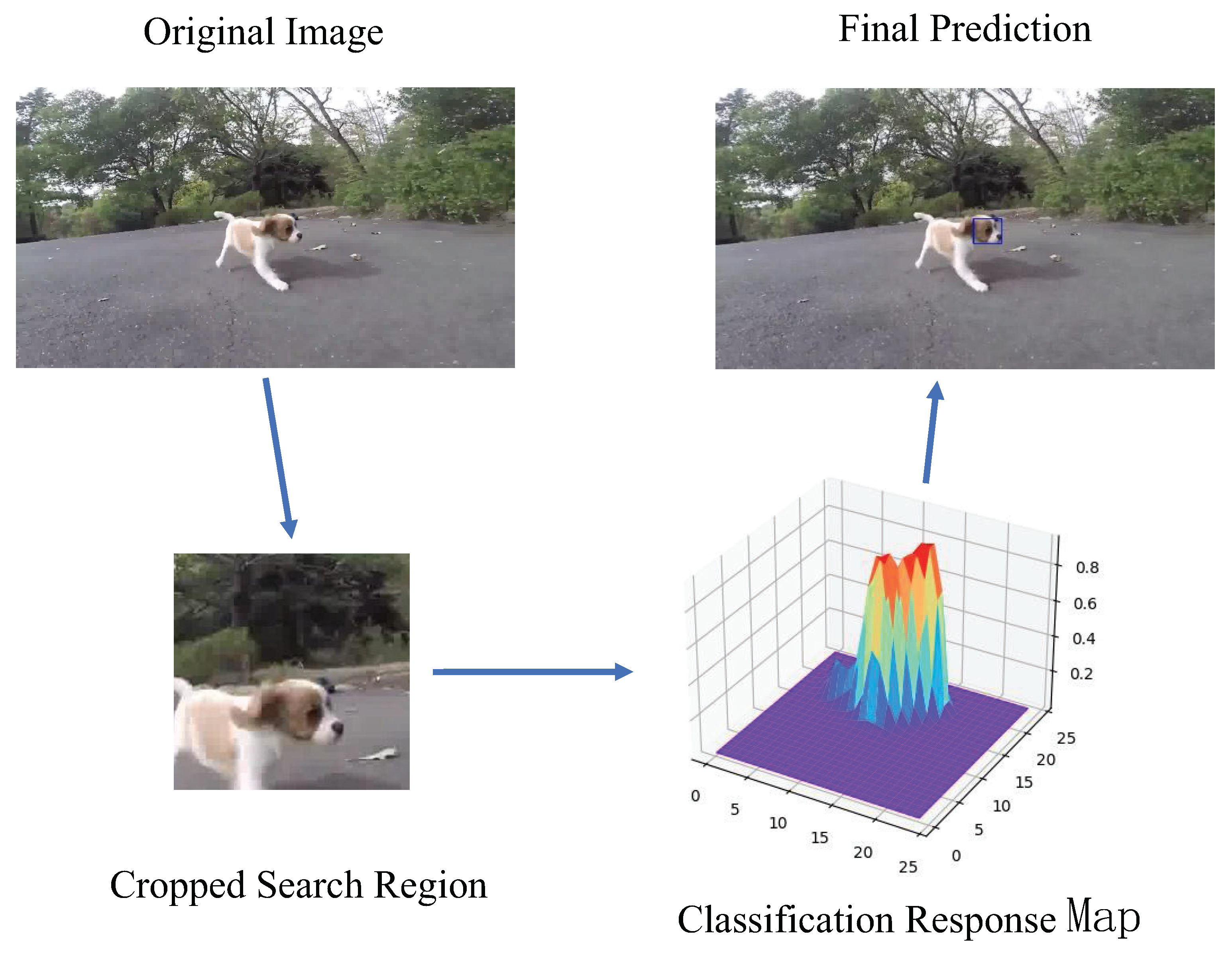
As shown in Figure 4, when the target scale increases after the template target is down-sampled by the backbone network, it will not be able to fully match the down-sampled features of the target in the search area and can only match local features. Such incomplete similarity matching of object information will cause ambiguity, causing the tracker to make wrong judgments and only return bounding boxes that contain object parts. As shown in Figure 5, the peak coverage of the target in the classification response map is large, indicating that the tracker judges this area to be a target. The final prediction result can only select the cell position corresponding to the peak in the classification response graph for regression, so only the local part of the target is regressed. Similarly, when the scale of the target is reduced, the down-sampling of the search area will include a lot of background information around the target, which will affect the prediction results of the tracker.
Combined with the above analysis, the main reason for the above impact is that the tracker cannot adapt to the change in the target’s scale, which leads to erroneous prediction results and makes the clipping strategy invalid, resulting in a vicious circle. On the one hand, the change in the target’s scale is usually accompanied by a change in appearance, shape, and action, which increases the difficulty faced by the Siamese network when attempting to accurately execute similarity matching. On the other hand, the change in target scale is reflected in the change in the number of pixels contained in the target in the original video frame, which also represents the change in the amount of target information contained in the video frame, which will have a great impact on similarity matching.

3. Our Method

This paper solves the problem of target scale change by fusing features at multiple different scales to reduce the impact of target scale changes. Moreover, the fused features include feature maps with detailed semantic information and feature maps with rich spatial information, further improving the model’s ability to depict the target object. In addition, our method improves the performance of the model when facing other challenges. At the same time, we use the 3D Max Filtering (3DMF) module to eliminate repeated predictions under multiple different scale features, improve the discrimination ability with respect to local area convolution, and further improve the precision and accuracy of the model.

3.1. The General Framework of the Algorithm

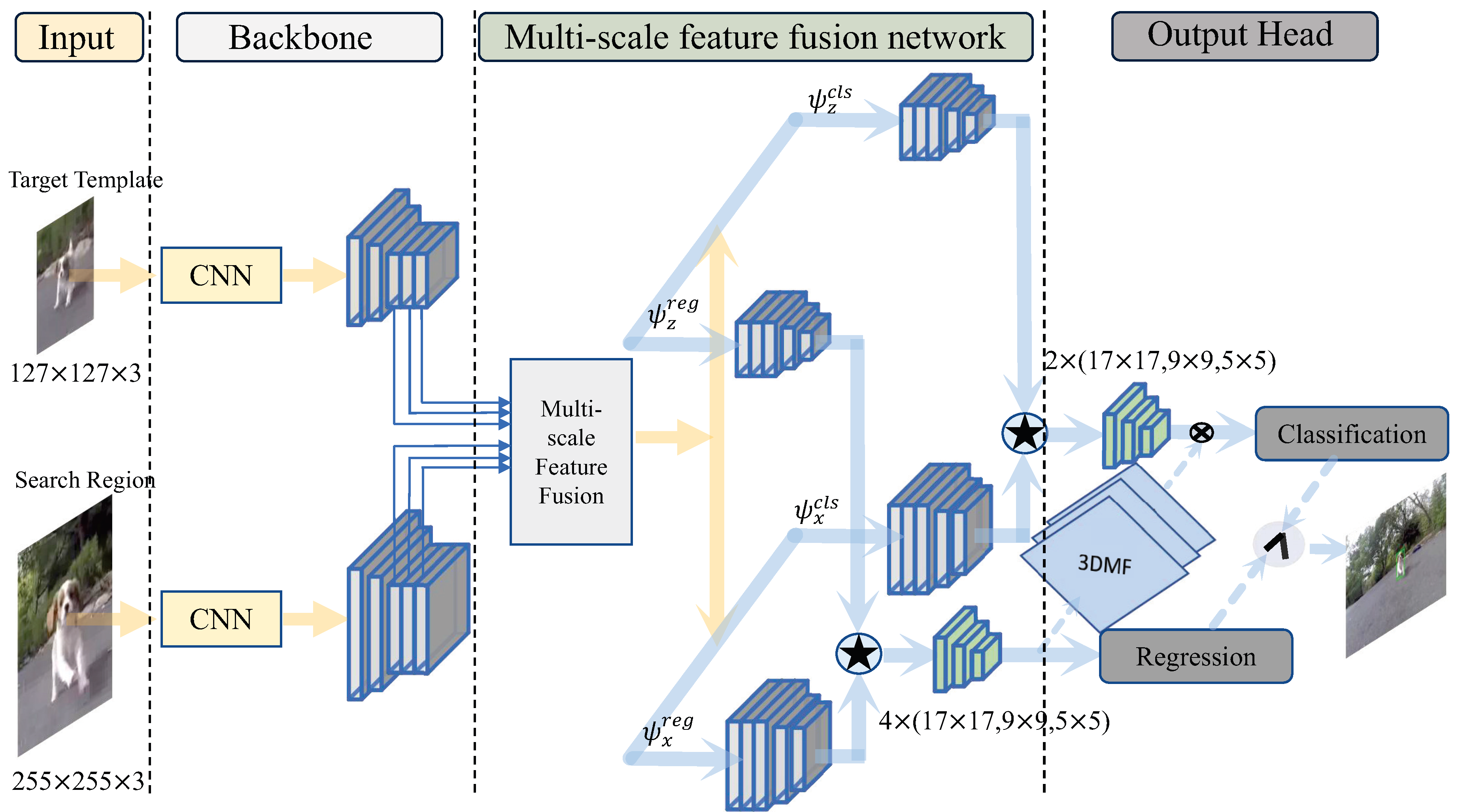
The algorithm framework of this paper is shown in Figure 6. It mainly includes four parts: an input, a backbone network, a multi-scale feature fusion network, and an output head. Among these parts, the input consists of two parts, namely, the target template ( 127 × 127 × 3 ) and the search area ( 255 × 255 × 3 ). The backbone network of the template branch and the backbone network of the search area branch share weights. A multi-scale feature fusion network is the method proposed in this paper, and its output contains two branches, which are used for classification and regression, respectively. In the output header section, we introduced additional 3D Max Filtering (3DMF).
First, the inputs from the template branch and the search branch are fed into the backbone network for feature extraction. This paper uses ResNet-50 as a backbone network. ResNet-50 employs continuous convolution steps to learn more and more abstract feature representations, but the feature resolution will be reduced after each layer of down-sampling. In order to ensure that there is enough spatial information to perform predictions for small objects, we removed the down-sampling operation in the last two convolutional blocks of ResNet-50, and the stride was set to 1. Meanwhile, to improve the receptive field, atrous convolution [26] is used in the last two convolutional blocks, and the dilation ratios are set to 2 and 4, respectively. Therefore, the resolution of the last three layers of the output features of the backbone network is the same.
Next, the last three layers of features extracted by the template branch and the search branch through the backbone network are sent to the multi-scale feature fusion network to obtain multi-scale features for classification and regression, respectively, and then perform cross-correlation operations (★ in Figure 6). The cross-correlation operation is performed separately for the features of the template branch and the search branch of the same size at the corresponding level. As shown in Figure 6, the template branch and the search branch have five layers of features for classification and regression, so the response map’s output after the cross-correlation operation should also have five layers. However, we adaptively fuse the first three layers of the same size, so the final classification and regression response maps have only three layers, with dimensions of 17 × 17 , 9 × 9 , and 5 × 5 , respectively. Each level of the classification response map includes two channels of foreground and background, and each level of the regression response map includes four channels of the regression vector.
Finally, the 3D Max Filtering (3DMF) module is applied to classification and the output response map, combining the predictions obtained through classification and regression to localize the target. The overall flow of the algorithm’s framework can be expressed as follows:
P l c l s = F φ z i c l s F φ x i c l s i = 3 , 4 , 5 P l r e g = F φ z i r e g F φ x i r e g i = 3 , 4 , 5
P w × h × 2 c l s a l l = l = 1 3 α l P l c l s , P 4 c l s , P 5 c l s P w × h × 4 r e g a l l = l = 1 3 β l P l r e g , P 4 r e g , P 5 r e g
In Equation (2), z and x are the inputs of the template branch and search branch, respectively. The function φ represents the feature extraction operation of the backbone network, and i = 3 , 4 , 5 denotes the last three layers that use the extracted features. The F function represents the multi-scale feature fusion operation adopted by the multi-scale feature fusion network. ★ indicates a cross-correlation operation. P l c l s and P l r e g represent the response maps output by the classification module and the regression module, respectively, after the cross-correlation operation. l = 1 , 2 , 3 , 4 , 5 means that the response map obtained at this time has five layers. Equation (3) is mainly used to weight the first three layers of the response map obtained earlier. Among them, α l , and β l are the weights corresponding to the response map of each level, which are optimized together with the network. P w × h × 2 c l s a l l and P w × h × 4 r e g a l l represent the final classification and regression response maps, containing three levels at different scales.

3.2. Multi-Scale Feature Fusion Network

In this paper, the backbone features at multiple scales are fused, and a feature pyramid with high-level semantics is constructed. The multi-scale feature fusion network we built can fuse low-resolution feature maps with detailed semantic information and high-resolution feature maps with rich spatial information with a few computations. The multi-scale feature fusion network can effectively fuse features at different scales to construct a feature pyramid and realize that each layer in the pyramid is a feature map with strong semantic information and precise location information. It improves the detection of small objects and solves the problem multi-scale object detection problem to a certain extent.
Although some methods in recent work have already used multi-scale feature fusion, we built our own multi-scale feature fusion network after analyzing the shortcomings of Siamese networks. Our proposed method built a novel network architecture, but other methods use the original FPN for multi-scale feature fusion, so our method is different from theirs. For example, in [27], the authors used the original FPN for multi-scale feature fusion but only output the score map at a single scale. Different from [27], we use our self-built multi-scale feature fusion network and output score maps at three different scales. The advantage of using score maps at multiple scales is that this strategy can provide more choices that the model can use to predict a target, and it greatly improves the model’s ability to cope with target scale changes.
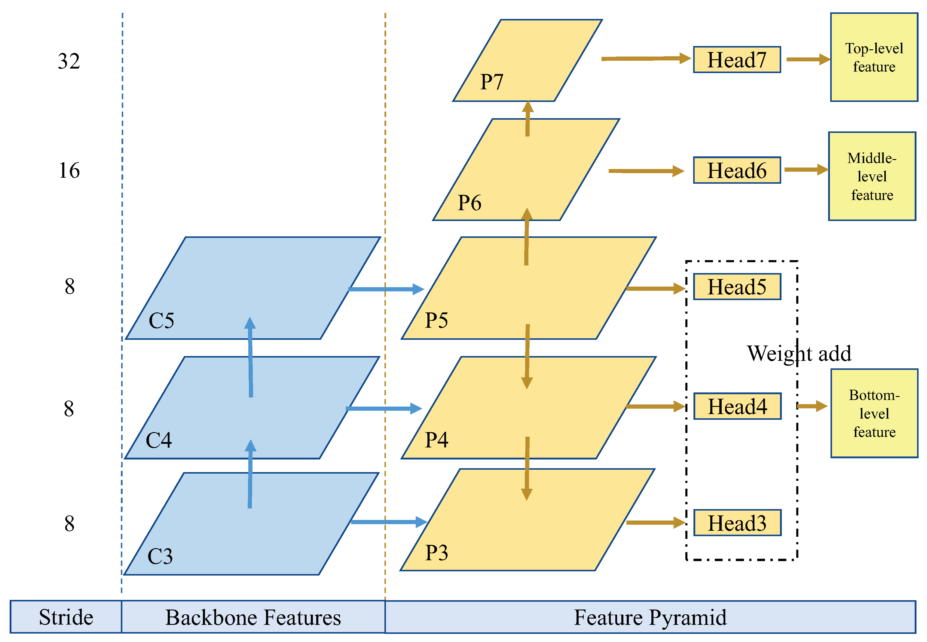
The multi-scale feature fusion network structure we built is shown in Figure 7. In the Figure, C3, C4, and C5 represent the last three layers of the backbone network feature map, and their down-sampling stride are the same, so the output feature scales of P3, P4, and P5 are the same. On this basis, P5 is continuously down-sampled to obtain the features of P6 and P7. Head3 to Head7 simultaneously receive feature pyramids from the template branch and the search branch and output classification and regression response maps. And no parameters are shared between them; each module is set up independently. Finally, via the multi-scale feature fusion network, the features at three scales are output.
The multi-scale feature fusion network shown in Figure 7 includes a bottom–up path on the left, a lateral connection in the middle, and a top–down path on the right. The bottom–up path on the left is the feed-forward computation of the backbone network, which computes a feature hierarchy consisting of feature maps at multiple scales. The top–down path on the right up-samples the spatially coarser but semantically stronger feature maps and is then augmented by laterally connecting features from the bottom–up path on the left. Each lateral connection incorporates feature maps of the same spatial size from the bottom–up path on the left and the top–down path on the right. After the above operations have been executed, the output feature map of each layer incorporates features of different scales and semantic strengths. Moreover, layers P6 and P7, which are obtained by continuing to down-sample P5, have stronger semantic features. When the target scale varies greatly, this semantic feature can be used to match the target.
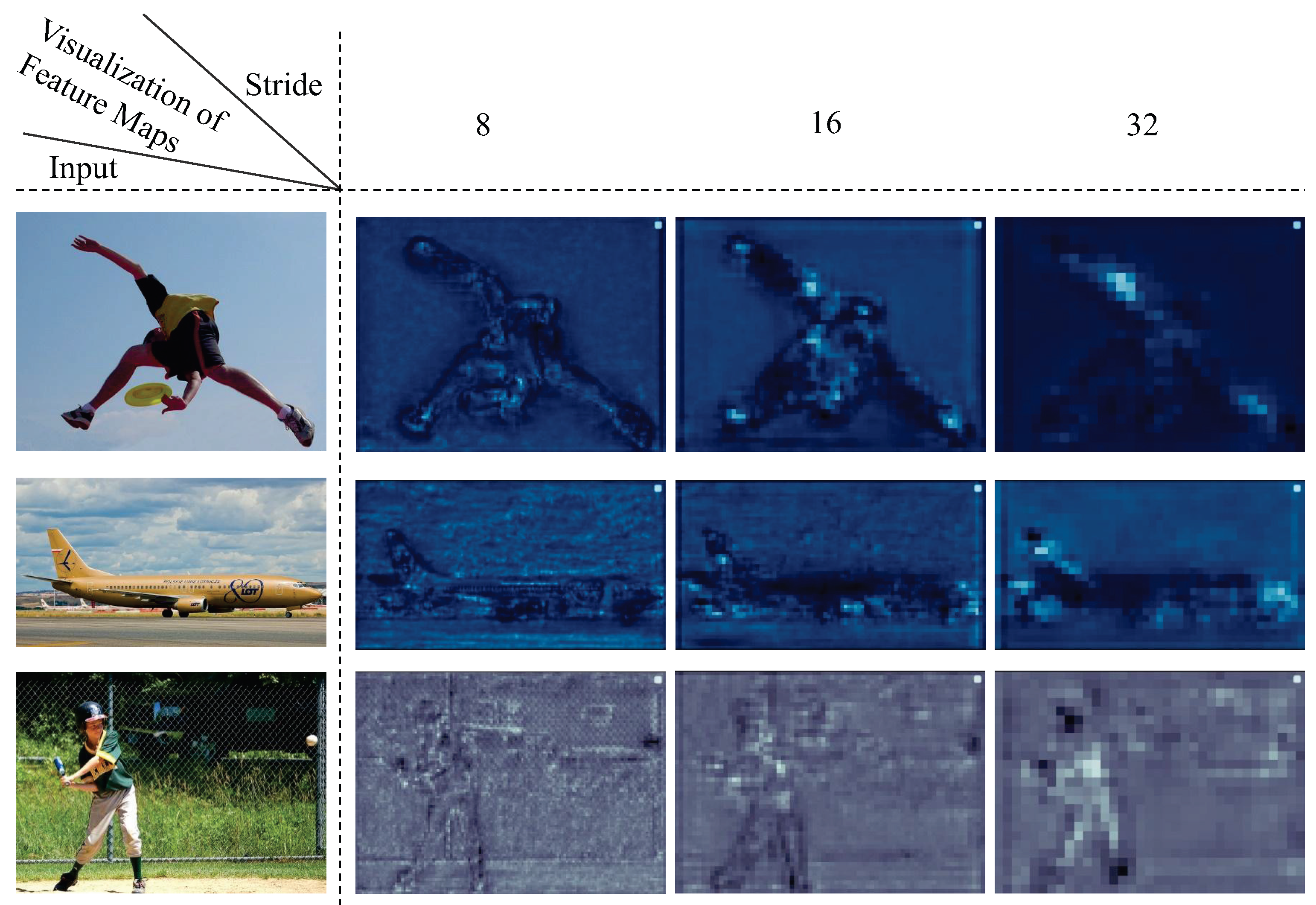
In order to more intuitively explain the characteristics of the output feature maps at different levels of the feature pyramid, we selected several original images from the COCO [28] dataset. These images was directly input into the multi-scale feature fusion network without cropping. Then, we visualized the feature maps output at different levels, as shown in Figure 8. It can be seen from the figure that the feature map located at the bottom layer of the feature pyramid (for which the stride is 8, corresponding to the bottom layer in Figure 7) is rich in target texture and spatial information. Generally, as the down-sampling stride increases, the resolution of the feature map will become smaller and smaller. At this time, the feature map will contain continuously less target texture and spatial information and will instead contain an increasingly more abstract semantic information. However, it can be seen from Figure 8 that the features at different levels of the feature pyramid contain the texture and spatial information of the target. Moreover, after multi-scale feature fusion, even the bottom layer of the feature pyramid contains the semantic information on the target.
Regarding the problem of target scale changes, if the target scale changes from small to large, then the top-level features of the feature pyramid can be used for matching. The feature pyramid is rich in target semantic features, and it also contains target texture and spatial information, which greatly improves the robustness of template target similarity matching. Moreover, the features at the top layer come from the deep network, the receptive field becomes larger, and the global information is more abundant. As the feature resolution decreases, the target scale gap narrows due to the deepening of the down-sampling degree. Similarly, if the target scale changes from large to small, then the features at the bottom of the feature pyramid can be used for matching. These features is rich in fine-grained information about the target and contains semantic information about the target; it comes from a shallow network; the resolution of the corresponding feature map is low; and the receptive field of a single pixel is relatively small, which allows for the capture of more information about small targets. Since the features of multiple scales are output through the multi-scale feature network, this network contains more information about the target object than the features at a single scale. So, the ability of the model to depict a target is improved. Even when faced with other challenges, such as blurring, lighting changes, etc., the accuracy of the model is still improved.

3.3. 3D Max Filtering Module

Although multi-scale feature fusion improves a model’s ability to depict a target, due to multiple scales accounted for, multiple levels (feature pyramids) of response maps of different scales are output. These response maps at different scales may produce repeated predictions for the target, thereby affecting the correct judgment of the model. To address this problem, we utilize the 3D Max Filtering (3DMF) module to suppress duplicate predictions.
The max filter is a rank-based nonlinear filter [29] that compensates for the discriminative power of convolutions in local regions. Furthermore, max filters have also been applied in keypoint-based detectors, such as CenterNet [18] and CornerNet [17], as an alternative to non-maximum suppression for post-processing, showing some potential for performing deduplication. However, maximum filtering can only be applied to single-scale features and cannot be considered comprehensively across multiple-scale features. 3D Max Filtering upgrades maximum filtering to a multi-scale version that can aggregate multi-scale features to suppress repeated detection. This module can exploit maximum filtering across scales to select predictions with the highest activation values in local regions and can enhance the ability to distinguish predictions.
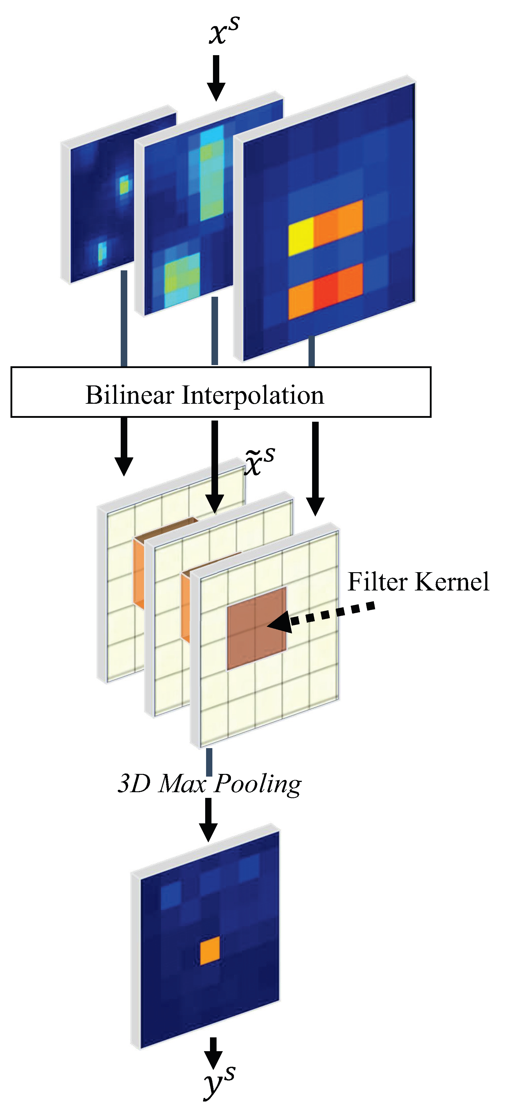
A flowchart depicting 3D Max Filtering is shown in Figure 9. This filtering method acts sequentially on different levels of the feature pyramid. Its input includes the feature map x s of the current level and the feature map of the nearest level adjacent to it. First, it is necessary to unify their sizes to the size of x s via bilinear interpolation:
x ˜ s = x ˜ s , k : = Bilinear x s x k k s T 2 , s + T 2
Among the terms listed above, s represents the different levels of the feature pyramid, and T represents the cross-level range of the input. We selected T = 3 . Next, it is necessary to perform a maximum pooling operation on x ˜ s in three-dimensional space, as shown in the following formula:
y i s = max k s T 2 , s + T 2 max j N i ϕ × ϕ x ˜ j s , k
Among the terms listed above, i represents the spatial position in the feature map of level s, and ϕ × ϕ is the spatial area centered on i, that is, the size of the filter kernel. We selected ϕ = 3 . y i s is the maximum value in the predefined three-dimensional domain. As shown in Figure 9, the final output feature map has the same shape as the input feature map x s . In addition, all modules in 3D Max Filtering are differentiable and can be trained together with the forward propagation process of the model network with very little computational consumption.

3.4. Design of Labels and Loss Functions

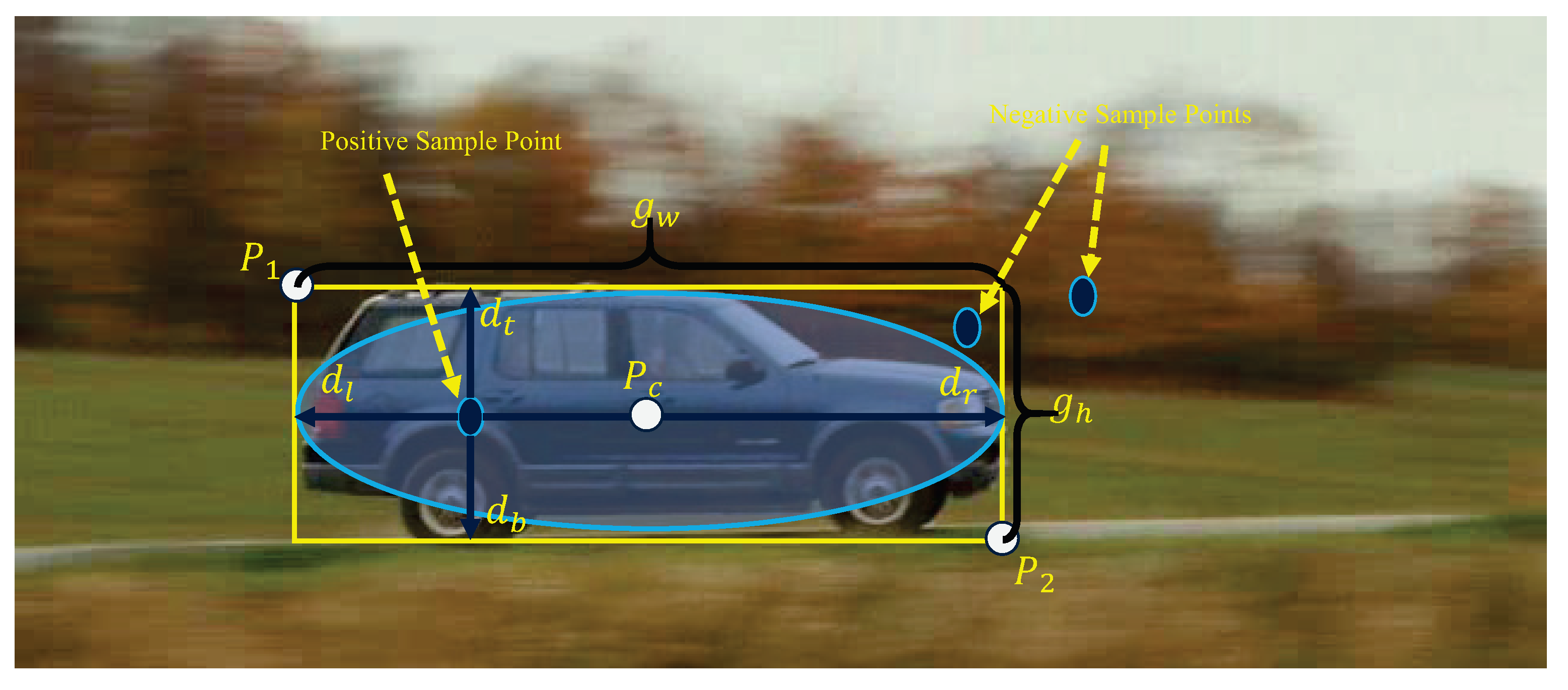
As shown in Figure 10, the objects in each search area are marked with ground-truth rectangles (the yellow rectangular frame in the figure). The width and height of the ground-truth rectangular box are represented by g w and g h , respectively, and the top left corner ( P 1 ), center-point ( P c ), and bottom right corner ( P 2 ) are represented by g x 1 , g y 1 , g x c , g y c , and g x 2 , g y 2 , respectively. After taking g x c , g y c as the center and g w 2 , g h 2 as the axis length, the resulting ellipse can be expressed as follows:
p i g x c 2 g w 2 2 + p j g y c 2 g h 2 2 = 1
If position p i , p j is inside the ellipse, it will be considered a positive sample; conversely, if it is outside the ellipse, it will be considered a negative sample. The reason for this design is that the bounding box of the object is not tight, and it is likely to contain the background in its corner. Use the position p i , p j of the positive sample to regress the bounding box. The goal of this regression is to determine the distance d l , d t , d r , d b from the position to the four sides of the rectangular box, as described in the following formula:
d l = p i g x 1 , d t = p j g y 1 , d r = g x 2 p i , d b = g y 2 p j ,
The classification loss function adopts Focal Loss [30], and its form is described in the following formula:
L c l s = 1 N p o s i , j α 1 p i , j γ log p i , j if labe l i , j = 1 1 α p i , j γ log 1 p i , j other
where i , j are the spatial position coordinates of the classification response map, p i , j is the classification score output by the model, N p o s is the total number of positive samples, and α and γ are the hyperparameters of Focal Loss; additionally, we selected α = 0.25 and γ = 2 .
The design of the regression loss function is shown in the following formula:
L r e g = 1 N p o s i , j L I o U d i , j , d i , j * if d i , j * > 0 0 other
where d i , j is the regression label, d i , j * is the regression vector predicted by the model, and L I o U = 1 I o U is the IoU loss. The total loss is defined as the weighted output of classification loss and regression loss:
L t o t a l = λ 1 L c l s + λ 2 L r e g
where λ 1 and λ 2 are weight proportions, and λ 1 = 1 and λ 2 = 1 are selected in the training stage.

4. Experiment

4.1. Implementation Details

4.1.1. Training Phase

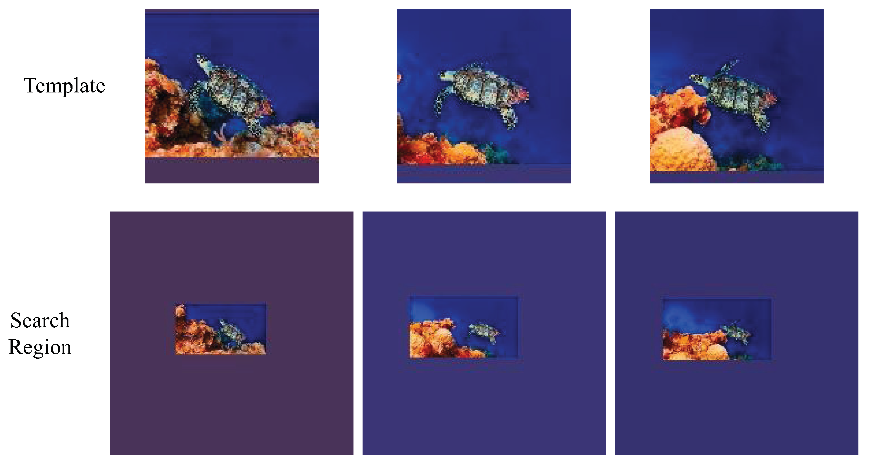
The backbone network of the architecture in this paper adopts the ResNet-50 structure, which was pre-trained through image classification tasks on ImageNet [31] dataset. This approach has been shown in [32,33] to be a very good way of initializing other tasks. We adopt COCO [28], GOT10K [34], and LaSOT [35] as the basic training sets. For the video datasets GOT10k and LaSOT, each video contained within them is cropped into template and search pairs frame by frame, as shown in Figure 11. For the image dataset COCO, all annotated objects contained in each image are individually cropped into template and search (the target is enclosed by a yellow rectangle) pairs, as shown in Figure 12. Additionally, translation, scale transformation, and color enhancement are carried out on the search image according to the uniform distribution, serving as a data enhancement operation, as shown in Figure 13.
In the training and testing stages, we adopted 127 pixels and 255 pixels as the template and search input image sizes, respectively. Due to limited resources, the training process of the model we built was carried out on two Nvidia RTX2080ti GPUs on a cloud server using Python’s Pytorch framework. During the training process, the backbone network was initialized with pre-trained weights, and a small batch of stochastic gradient descent (SGD) with a batch size of 28 was used for training for a total of 20 epochs. The initial learning rate was 0.001, which gradually increased to 0.005 in the first five epochs for a warm-up. The learning rate of the last 15 epochs decayed exponentially from 0.005 to 0.00005, allowing the network to converge better. In the first 10 epochs, the parameters of the backbone network were frozen, and only the multi-scale feature fusion network and the output head network part were trained. In the last 10 epochs, we unfroze the last three layers of the backbone network ResNet-50, added them to the training set, and fine-tuned the backbone network part at the then current one-tenth learning rate. The total training time was 72 h.

4.1.2. Inference Phase

After the 3D Max Filtering module has been applied to all levels of the regression output, it is multiplied with the classification score map to obtain the final classification prediction output. The location of the maximum score in all hierarchical response maps of the classification output is then selected and combined with the regression vector at this location to regress the target bounding box. Since regression vectors at different scales of multiple levels are output, the regression ranges of different levels are different, so the regression vectors of each level use the scaling factor scale to scale the regression results (via multiplication by s c a l e ). The scaling factor scale is used as a parameter incorporated in the training of the network.

4.1.3. Evaluation

We performed the test using four tracking benchmarks: OTB2015 [36], VOT2016 [37], VOT2018 [38], and GOT10K [34]. On this basis, the tracker we builtwas compared with many advanced trackers, including with respect to various evaluation metrics and performance comparisons under different challenge attributes.

4.2. Ablation Experiment

In order to prove the effectiveness of the method we designed, we conducted relevant ablation experiments based on the VOT2016 dataset. We built a baseline network, for which we removed the multi-scale feature fusion network and 3D max Filtering network we developed, and we used the remaining parts to build this network. As shown in Table 1, A and EAO are the evaluation metrics of the VOT dataset, representing Accuracy and Expect Average Overlap, respectively. The EAO measures precision; the larger the value, the higher the degree of precision. “✓” in the table indicates that the corresponding method was used. Accuracy is calculated determining the average IoU of valid frames; the larger the value, the higher the accuracy. The calculation method for IoU is expressed as follows:
I o U = A B A B
where, as shown in Figure 14, A represents the ground truth bounding box of the target (as shown in the yellow rectangle in the figure), B represents the bounding box predicted by the algorithm (as shown in the blue rectangle in the figure), and IoU is their Intersection over Union.
By comparing the results of Experiment 1 and Experiment 2, we found that after applying the multi-scale feature fusion network we designed to the baseline, the precision of the algorithm increased by 7.6%, while its accuracy increased by 1.7%. These results show that the multi-scale feature fusion network we designed yields very good results. In experiment 3, after continuing to introduce the ellipse label strategy, the performance of the algorithm was slightly improved. The improvement in precision reached 9.0%, and the improvement in accuracy reached 1.8%. Compared with the performance observed before this strategy was used, the precision of the algorithm improved by 2.4%, and its relative accuracy improved by 0.1%. When the 3D Max Filtering module was used in Experiment 4, the precision of the algorithm increased by 17.5%, and its accuracy increased by 3.2%. Compared with the performance observed before this strategy was used, the performance of the algorithm has been greatly improved, presenting a relative improvement in precision of 8.3% and a relative improvement in accuracy of 1.4%. This result shows that the 3D Max Filtering module has played a very important role.
For the ellipse label, the corresponding label is the rectangular label; that is, as long as the points located in the ground-truth rectangular box are considered positive sample points, the points outside the ground-truth rectangular box are negative sample points (refer to Figure 10). The ellipse label strategy slightly improves the performance of the algorithm because the sampling step size and the number of labels are different for different levels of classification response maps. The large response map at the bottom has a large number of positive samples. On the contrary, the small response map at the top has a small number of positive samples and a large receptive field. While the coverage of the rectangular box is great, it is likely that there is a lot of background in the corner. If the points in the small-scale response map of the top layer are incorrectly assigned as positive sample labels because they are situated in the corner of the rectangular box, this will cause the model to erroneously learn this layer, which will have an impact on the model’s output. Therefore, the choice of label design strategy will also have a certain impact. The 3D Max Filtering module can effectively suppress repeated predictions at different levels, so the precision and accuracy of the model are correspondingly improved.

4.3. Comparison with Other Advanced Trackers

4.3.1. Comparison Using the OTB2015 Benchmark Dataset

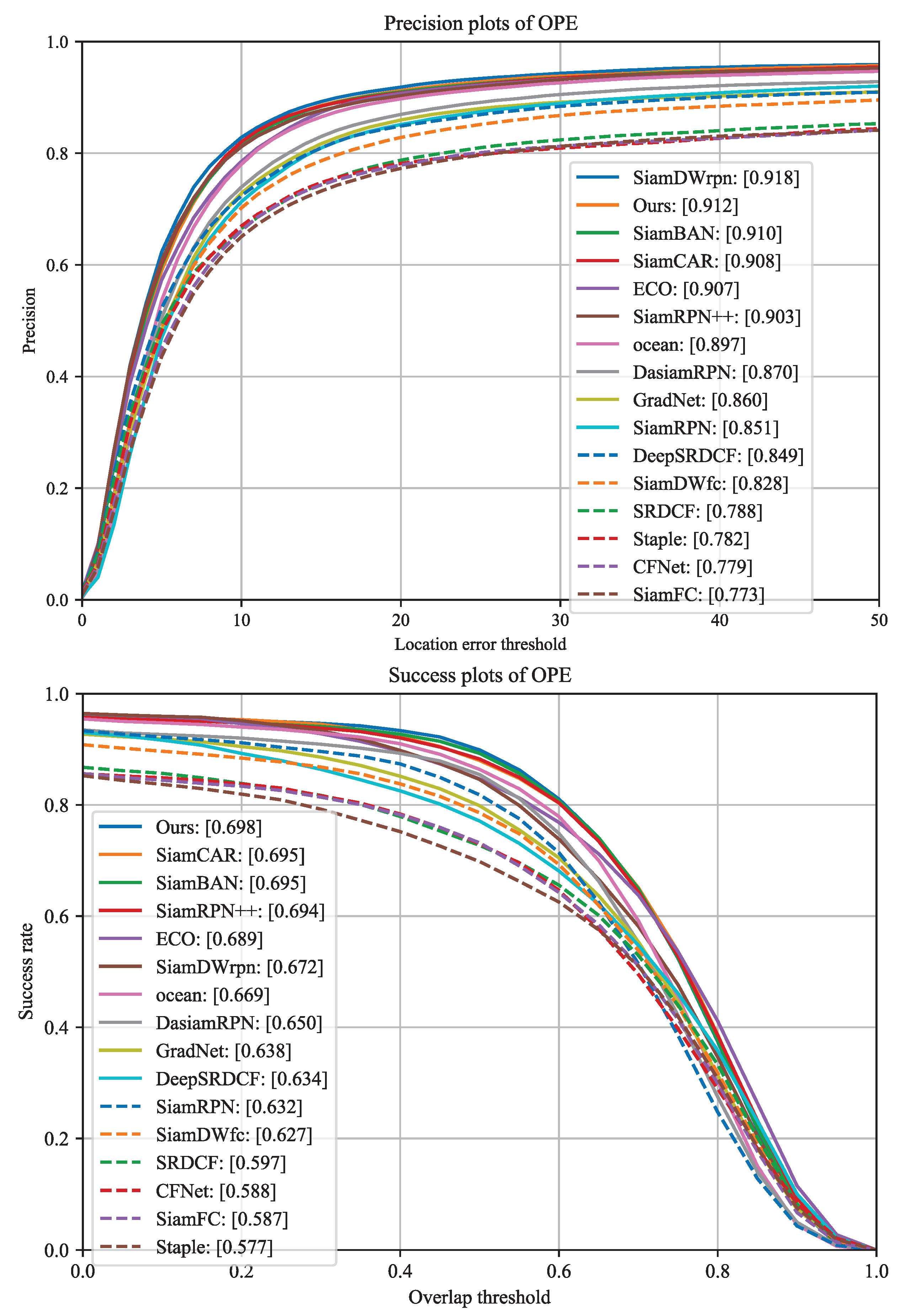
The OTB100 [36] dataset, proposed in 2015, is one of the most extensive test benchmarks for visual object tracking, consisting of 100 well-annotated video sequences. The evaluation metrics of the OTB100 dataset mainly include precision and success rate. Precision is mainly measured in terms of the center position error, wherein the Euclidean distance between the center-point of each frame Ground Truth and the center-point of the bounding box output by the algorithm is calculated as the center-point error of each frame. Subsequently, the center-point errors of all frames are averaged; the larger the value, the larger the error. When visualizing, the ordinate is the percentage of frames in which the center-point of the algorithm output bounding box and the center-point of the Ground Truth are less than the specified threshold when compared to the total number of frames. The abscissa is the specified threshold, which ranges from 0 to some maximum distance. The final curve drawn is a precision plot. The success rate is mainly measured using IoU.
Using the OTB2015 benchmark as a reference, we compare our proposed algorithm with several state-of-the-art trackers, including many Siamese-based trackers and other types of trackers. As shown in Figure 15, in terms of precision, our algorithm reached 91.2%, surpassing many excellent tracking algorithms and ranking among the leading positions (it is only 0.6% away from first place). In terms of success rate, our method achieves 69.8%, which places it in the leading ranks. These results show that our proposed method effectively improves the performance of Siamese-network-based trackers.

4.3.2. Comparison Using the VOT2016 Benchmark Dataset

VOT is a public test benchmark dataset that is widely used. It has been updated every year since VOT2013, and its latest update was VOT2020. The tracking difficulty of the VOT dataset is much higher than that of the OTB dataset. This dataset provides a lot of tracking scenarios involving more complex factors such as small targets and non-rigid object motion. Following the release of VOT2018, this dataset also provides a sub-dataset specifically used to evaluate long-term tracking algorithms. And the tracking target marked in OTB only uses the traditional vertical rectangular bounding box as the Ground Truth of the target, while in the current version of the VOT dataset, the minimum circumscribed rectangle of the tracking target is used as the Ground Truth of the target. In the latest data set, the mask of the tracking target is also provided as Ground Truth for evaluation by some algorithms that combine object tracking and object segmentation.
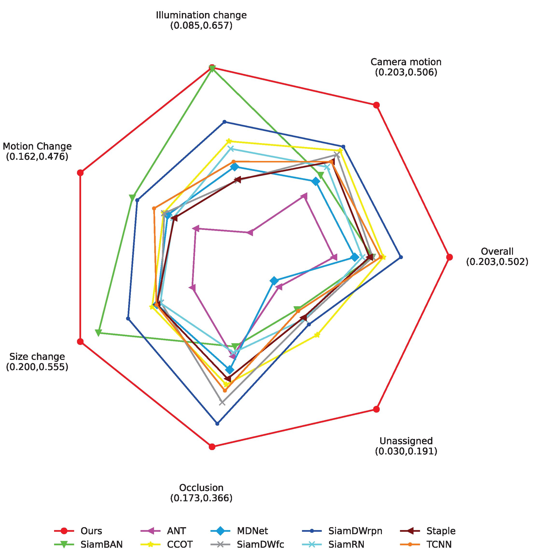
The performance of our method in relation to VOT2016 [37] is compared with several state-of-the-art trackers in Table 2, where the arrows indicate the direction of superior performance. It can be seen that our method surpasses many excellent Siamese-network-based trackers in terms of accuracy, precision, and robustness and is in the leading ranks. In addition, we also made a precise comparison of the precision values in relation to the various challenging attributes of VOT2016, as shown in Figure 16. These challenging attributes include motion changes, illumination changes, camera motion, unassigned targets, occlusion, and size changes. The values in brackets represent the minimum and maximum EAO scores of the trackers participating in the comparison in relation to each challenge attribute, and the average value of the EAO under all challenge attributes of each tracker is the EAO of the tracker in Table 2. Therefore, in Figure 16, the precision performance of each tracker with respect to each challenge attribute is obvious. It can be seen that the precision of our proposed method reached the leading levels for each challenge attribute, especially with respect to the aspect of size change, where precision reached a very high value of 55.5%, which is a level that the other trackers did not reach. Moreover, the accuracy of illumination change reached 65.7%, far exceeding other trackers except SiamBAN. Under the challenging conditions of motion change, camera motion, unassigned targets, and occlusion, our proposed method outperforms the other trackers. In summary, our proposed method not only improves the ability of Siamese-network-based trackers to cope with the challenge of scale variation but also improves their performance in the face of other challenges to a certain extent.

4.3.3. Comparison Using the VOT2018 Benchmark Dataset

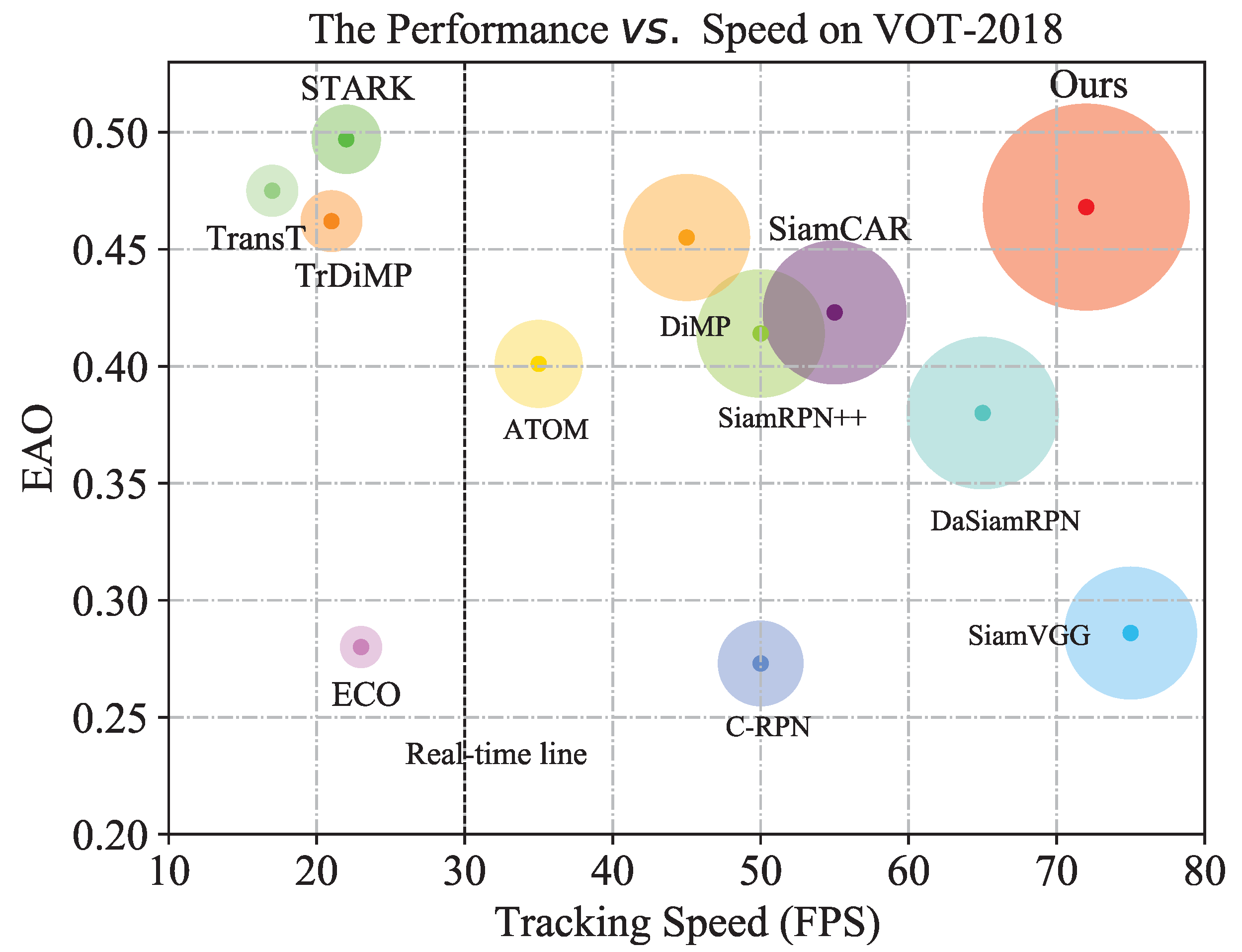
Figure 17 intuitively shows the comparison results in relation to the VOT2018 [38] dataset. It comprehensively considers EAO and speed performance, which are represented by the horizontal and vertical axes, respectively. The real-time line in the figure indicates the limit of real-time speed. Speed performance dominates this comparison. In the figure, the better the overall performance of the algorithm, the closer it is to the upper right corner, and the larger the area of the circle representing the performance of the algorithm. On the contrary, the worse the comprehensive performance of the algorithm, the closer it is to the lower left corner (which is the coordinate origin), and the smaller the area of the circular area representing the comprehensive performance of the algorithm. It can be seen from Figure 13 that our proposed method shows superior comprehensive performance, and its tracking speed is far beyond the real-time speed. In addition, the EAO score of our proposed method is also in the leading position compared to the other excellent trackers. While transformer-based trackers such as TransT [45], STARK [46], and TrDiMP [47] have good EAO scores, their speed performance lags behind that of Siamese-network-based trackers and does not meet the real-time speed requirements. It can also be clearly seen from the figure that they are all distributed in the upper left corner, which also reflects the disadvantage of the transformer-based tracker, that is, its tracking speed is slow. The other trackers based on Siamese networks can meet the requirements of real-time speed.

4.3.4. Comparison Using the GOT10K Benchmark Dataset

GOT10K [34] is a large-scale, short-term object-tracking dataset based on WordNet that covers 560 categories of common outdoor moving objects and can be used for unified training and the evaluation of depth tracking. GOT10K requires the algorithms participating in comparison to use its own training dataset for training alone, followed by its own test set for testing.
In Table 3, we compare our proposed method with other trackers, and the main types of algorithms involved in the comparison are based on Siamese networks. Compared with state-of-the-art Siamese network trackers such as SiamCAR [21] and SiamBAN [22], our method achieves far superior performance. Regarding the Average Overlap (AO) score, our method achieves a value of 64.9%, which surpasses many excellent tracking algorithms, placing it in the leading ranks.

4.3.5. Tracking Efficiency Analysis

The analysis of tracking efficiency is very important because it is related to the practical application of a tracker. In this comparison of tracking efficiency, we contrast our method with some state-of-the-art Siamese-network-based trackers. For fairness, the tracking efficiency evaluation of each tracker was performed on one computer with an NVIDIA Quadro P4000 GPU and 64 GB of RAM memory. We evaluated the tracking speed, the number of parameters, and the number of floating point operations (FLOPs) in the tracking model of the trackers involved in the comparison, as shown in Table 4. Among these parameters, tracking speed is a very important indicator related to practical applications, and it is calculated by determining the average number of frames processed by a tracker in one second. The number of parameters is another important efficiency metric in deep-learning-based tracking methods as a model with a low number of parameters is efficient in terms of hardware and consumes less RAM, so it can work on small devices like mobiles and tablets. The number of parameters of a tracking model is the total number of parameters passed to the optimizer, and in most cases, it does not depend on the input size of the tracking method. We consider the number of floating point operations (FLOPs) as a third metric for measuring the efficiency of the tracking models. The number of FLOPs of a CNN-based tracker depends on the tracking model and the corresponding search image size since object template features are only computed in the first frame of the tracking sequence.
As can be seen from Table 4, the tracking speed of our method surpasses that of many excellent trackers and achieves real-time speed. It can be seen that the tracking efficiency of SiamDW [13] is outstanding, and it achieves high-efficiency results, with 52.58 FPS of tracking speed and 2.46 million parameters. SiamGAT [50] achieves 41.99 FPS of tracking speed with 14.23 million parameters. The tracker we built achieved a tracking speed of 45.02 FPS with 59.77 million parameters and 59.34 gigaFLOPs and also showed good tracking efficiency. The tracking speeds of SiamGAT and SiamFC++ are similar to those of our model, but for the AO scores of GOT10k, they are 62.7 and 59.5, while our AO score is 64.9, surpassing them by 2.2% and 5.4%, respectively. Although our model’s precision when applied to OTB100 was inferior to that achieved by SiamGAT, the gap in performance was only 0.4%. Moreover, the challenge of the video sequence used for testing using the OTB00 dataset is too saturated, and it is difficult to achieve further improvement. SiamRN outperformed our method by 1.9% in precision when applied to OTB100, but its tracking speed was nowhere near that achieved by our model.

4.3.6. Analysis and Conclusion of Comparison

In this section, we compare many other state-of-the-art trackers, including many based on Siamese networks. They are all members of the Siamese-based tracker family and have made important contributions to the performance improvement and development of Siamese-based trackers. Our proposed method is also a Siamese-based tracking method, but our method outperforms the others within this group. So, using these methods as reference benchmarks, our proposed method further improves the performance of Siamese-based trackers.

4.4. Demonstration and Comparison of Actual Effects

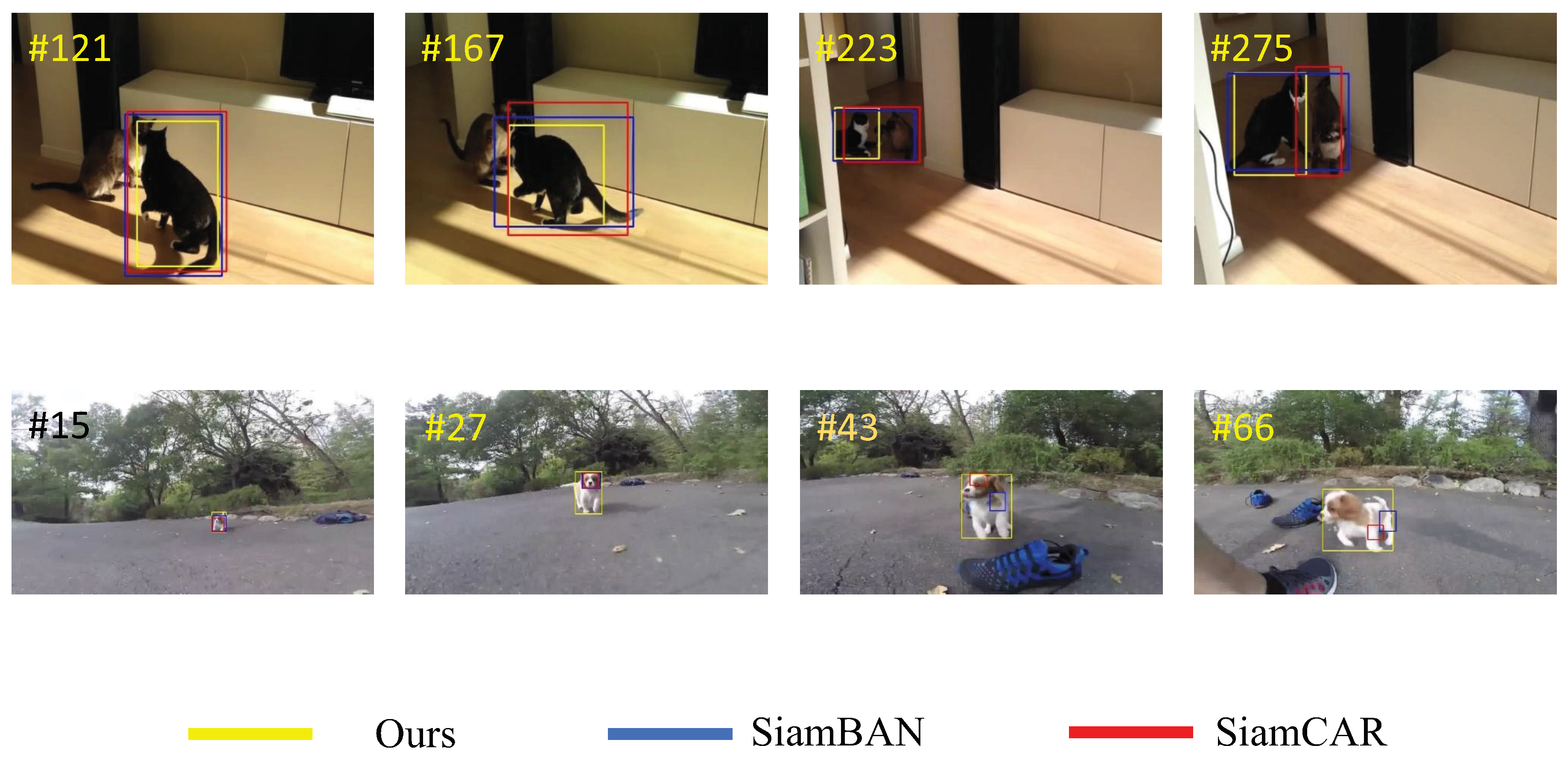
As shown in Figure 18, we selected two video sequences from VOT2016 and GOT10K with object scale variation properties and used them to compare the performance of the trackers. We compared the performance of our tracker with two state-of-the-art Siamese network trackers, SiamBAN and SiamCAR. The yellow rectangular box in the figure is the tracking result of our proposed algorithm; the blue box is the tracking result of SiamBAN; and the red one is the tracking result of SiamCAR. In the first scene, the target moves from near to far from the camera, and its scale changes from large to small. In the beginning, all the trackers were able to successfully locate the target. However, it can also be seen from the figure that, compared with the other two state-of-the-art trackers, the rectangular box generated by the tracker we built is tighter, which shows that the tracking precision of our tracker is higher than that of the other methods. When the target continued to move away from the camera, as shown in frame 233 in the figure, our tracker still successfully followed the target. However, the other two trackers confused the target with other objects, which greatly affected their tracking precision and accuracy. As shown in the scene in frame 275 of the figure, the SiamCAR tracker produced tracking drift, and the rectangular frame it generated drifted toward other objects. This means that it lost track of the target, which, in turn, led to tracking failure. The SiamBAN tracker confused the target with other objects. However, our tracker still managed to follow the target.
In the second scene in Figure 18, the target approaches the camera from far away, and the scale of the target gradually increases from small to large. It can be seen that in the beginning, the scale of the target does not change very much, and all the trackers can follow the target at this time. However, as time goes by, the scale of the object changes more and more, and the other trackers can no longer detect the object completely. It can be seen from the figure that the tracking results yielded by SiamCAR and SiamBAN fall in the local area of the target, resulting in tracking failure. However, our tracker can still detect a complete target, and the generated tracking result completely surrounds the target object. This demonstration of the models’ practical application shows that the algorithm we proposed improves the performance of the tracker based on the Siamese network, especially in the face of target scale change, which makes the tracker based on the Siamese network more robust.

5. Conclusions and Future Work

This paper first introduced the basic Siamese tracking framework, comprehensively analyzed the impact of object scale changes on Siamese trackers, and summarized the reasons for the latter. In this paper, the ability of the model to depict a target was improved by fusing the features of multiple different scales, thereby compensating for the shortcomings of the Siamese network tracker to a certain extent. At the same time, we used the 3D Max Filtering module to suppress repeated predictions under different scale features, further improving the precision and accuracy of the model. After multi-scale feature fusion, the features at different scales contained more valuable information, and the model’s ability to distinguish features was greatly enhanced. Different from previous Siamese network trackers, our algorithm outputs response maps at multiple scales, greatly improving the robustness and precision of the model. Our extensive experiments on multiple tracking benchmark datasets demonstrated that our proposed method outperforms many state-of-the-art trackers and ranks among the leaders. Our ablation experiments showed that the methods we designed can achieve good results.
In future work, we will continue to work on compensating for the shortcomings of Siamese-network-based trackers and further improving their performance. Most of the Siamese-network-based trackers are based on CNNs. CNN-based trackers have their own limitations; that is, they can only focus on local information and cannot model global information. A Siamese-network-based tracker can further amplify this shortcoming of CNNs (as described in Section 2.2 of this paper). Although this paper compensates for this defect to a certain extent by adopting the method of multi-scale feature fusion, by using features at multiple scales, the Siamese-network-based tracker can utilize more global information. But is there a better solution? This will be the direction of our further research. Today’s popular Transformer can learn global context information, but it will also require additional calculations, resulting in a serious drop in tracking speed. So, it is our next research topic to improve the modeling ability of the global context for Siamese-network-based trackers without affecting their speed performance.

Author Contributions

Conceptualization, J.Z. and D.N.; methodology, J.Z. and D.N.; software J.Z.; validation, J.Z. and D.N.; investigation, D.N.; formal analysis, J.Z.; resources, D.N.; writing—original draft preparation, J.Z.; writing—review and editing, D.N.; visualization, J.Z.; supervision, D.N. All authors have read and agreed to the published version of the manuscript.

Funding

This work was supported by the National Key Research and Development Program of China (No.2019YFF0302203) and the Fundamental Research Funds for the Central Universities: (No.N2304006).

Institutional Review Board Statement

Not applicable.

Informed Consent Statement

Not applicable.

Data Availability Statement

The datasets we used are all open public data benchmarks, including COCO, GOT10K, LaSOT, VOT2016, VOT2018, and OTB2015, and the relevant addresses have been attached in the references in the text. Relevant code can be obtained at https://github.com/long-wa/MFF-SNT, accessed on 10 July 2023.

Conflicts of Interest

The authors declare no conflict of interest.

References

  1. Jha, S.; Seo, C.; Yang, E. Real time object detection and tracking system for video surveillance system. Multimed. Tools Appl. 2021, 80, 1–16. [Google Scholar] [CrossRef]
  2. Premachandra, C.; Ueda, S.; Suzuki, Y. Detection and Tracking of Moving Objects at Road Intersections Using a 360-Degree Camera for Driver Assistance and Automated Driving. IEEE Access 2020, 99, 21–56. Available online: https://ieeexplore.ieee.org/document/9146556 (accessed on 10 July 2023). [CrossRef]
  3. Liu, Y.; Sivaparthipan, C.B.; Shankar, A. Human–Computer Interaction Based Visual Feedback System for Augmentative and Alternative Communication. Int. J. Speech Technol. 2022, 25, 305–314. Available online: https://link.springer.com/article/10.1007/s10772-021-09901-4 (accessed on 10 July 2023).
  4. Wang, H.; Deng, M.; Zhao, W. A Survey of Single Object Tracking Algorithms Based on Deep Learning. Comput. Syst. Appl. 2022, 31, 40–51. [Google Scholar]
  5. Meng, W.; Yang, X. A Survey of Object Tracking Algorithms. IEEE/CAA J. Autom. Sin. 2019, 7, 1244–1260. [Google Scholar]
  6. Bertinetto, L.; Valmadre, J.; Henriques, J.F.; Vedaldi, A.; Torr, P.H. Fully-convolutional siamese networks for object tracking. In Proceedings of the 14th European Conference on Computer Vision, Amsterdam, The Netherlands, 11–14 October 2016; pp. 850–860. [Google Scholar] [CrossRef]
  7. Qing, G.; Wei, F.; Ce, Z.; Rui, H.; Liang, W.; Song, W. Learning Dynamic Siamese Network for Visual Object Tracking. In Proceedings of the IEEE International Conference on Computer Vision, Venice, Italy, 22–29 October 2017; pp. 1763–1771. Available online: https://ieeexplore.ieee.org/abstract/document/8237458 (accessed on 10 July 2023).
  8. Wang, Q.; Teng, Z.; Xing, J.; Gao, J.; Hu, W.; Maybank, S. Learning attentions: Residual attentional siamese network for high performance online visual tracking. In Proceedings of the IEEE Conference on Computer Vision and Pattern Recognition, Salt Lake City, UT, USA, 18–23 June 2018; pp. 4854–4863. Available online: https://ieeexplore.ieee.org/document/8578608 (accessed on 10 July 2023).
  9. Li, B.; Yan, J.J.; Wu, W.; Zhu, Z.; Hu, X.L. High performance visual tracking with siamese region proposal network. In Proceedings of the 2018 IEEE Conference on Computer Vision and Pattern Recognition, Salt Lake City, UT, USA, 18–22 June 2018; pp. 8971–8980. Available online: https://ieeexplore.ieee.org/document/8579033 (accessed on 10 July 2023).
  10. Ren, S.; He, K.; Girshick, R.; Sun, J. Faster R-CNN: Towards real-time object detection with region proposal networks. Adv. Neural Inf. Process. Syst. 2015, 31, 91–99. [Google Scholar] [CrossRef] [PubMed]
  11. Li, B.; Wu, W.; Wang, Q.; Zhang, F.Y.; Xing, J.L.; Yan, J.J. SiamRPN++: Evolution of siamese visual tracking with very deep networks. In Proceedings of the 2019 IEEE Conference on Computer Vision and Pattern Recognition, Long Beach, CA, USA, 15–20 June 2019; pp. 4282–4291. [Google Scholar] [CrossRef]
  12. Wang, Q.; Zhang, L.; Bertinetto, L.; Hu, W.; Torr, P.H. Fast online object tracking and segmentation: A unifying approach. In Proceedings of the IEEE/CVF conference on Computer Vision and Pattern Recognition, Long Beach, CA, USA, 15–20 June 2019; pp. 1382–1383. Available online: https://ieeexplore.ieee.org/document/8953931 (accessed on 10 July 2023).
  13. Zhang, Z.; Peng, H. Deeper and wider siamese networks for real-time visual tracking. In Proceedings of the IEEE/CVF Conference on Computer Vision and Pattern Recognition, Long Beach, CA, USA, 15–20 June 2019; pp. 4591–4600. Available online: https://ieeexplore.ieee.org/document/8953458 (accessed on 10 July 2023).
  14. He, K.; Zhang, X.; Ren, S.; Sun, J. Deep residual learning for image recognition. In Proceedings of the IEEE Conference on Computer Vision and Pattern Recognition, Las Vegas, NV, USA, 27–30 June 2016; pp. 770–778. Available online: https://ieeexplore.ieee.org/document/7780459 (accessed on 10 July 2023).
  15. Xie, S.; Girshick, R.; Doll’ar, P.; Tu, Z.; He, Z. Aggregated residual transformations for deep neural networks. In Proceedings of the IEEE Conference on Computer Vision and Pattern Recognition, Honolulu, HI, USA, 21–26 June 2017; pp. 1492–1500. [Google Scholar] [CrossRef]
  16. Andrew, G.; Zhu, M.; Bo, C.; Kalenichenko, D.; Wang, W.; Weyand, T.; Andreetto, M.; Adam, H. MobileNets: Effificient convolutional neural networks for mobile vision applications. arXiv 2017, arXiv:1704.04861. [Google Scholar] [CrossRef]
  17. Law, H.; Deng, J. Cornernet: Detecting objects as paired keypoints. In Proceedings of the European Conference on Computer Vision (ECCV), Munich, Germany, 8–14 September 2018; pp. 734–750. [Google Scholar] [CrossRef]
  18. Zhou, X.; Wang, D.; Krähenbühl, P. Objects as points. arXiv 2019, arXiv:1904.07850. [Google Scholar] [CrossRef]
  19. Tian, Z.; Chu, X.; Wang, X.; Wei, X.; Shen, C. Fcos: Fully convolutional one-stage object detection. In Proceedings of the IEEE/CVF International Conference on Computer Vision, Seoul, Republic of Korea, 27 October–2 November 2019; pp. 9627–9636. [Google Scholar] [CrossRef]
  20. Xu, Y.; Wang, Z.; Li, Z.; Yuan, Y.; Yu, G. Siamfc++: Towards robust and accurate visual tracking with target estimation guidelines. In Proceedings of the AAAI Conference on Artificial Intelligence, New York, NY, USA, 7–12 February 2020; pp. 12549–12556. [Google Scholar] [CrossRef]
  21. Guo, D.; Wang, J.; Cui, Y.; Wang, Z.; Chen, S. SiamCAR: Siamese fully convolutional classification and regression for visual tracking. In Proceedings of the IEEE/CVF Conference on Computer Vision and Pattern Recognition, Seattle, WA, USA, 13–19 June 2020; pp. 6269–6277. Available online: https://ieeexplore.ieee.org/document/9157720 (accessed on 10 July 2023).
  22. Chen, Z.; Zhong, B.; Li, G.; Zhang, S.; Ji, R. Siamese box adaptive network for visual tracking. In Proceedings of the IEEE/CVF Conference on Computer Vision and Pattern Recognition, Seattle, WA, USA, 13–19 June 2020; pp. 6668–6677. Available online: https://ieeexplore.ieee.org/document/9157457 (accessed on 10 July 2023).
  23. Zhang, Z.; Peng, H.; Fu, J.; Li, B.; Hu, W. Ocean: Object-aware anchorfree tracking. In Proceedings of the Computer Vision–ECCV 2020: 16th European Conference, Glasgow, UK, 23–28 August 2020; pp. 771–787. [Google Scholar] [CrossRef]
  24. Wang, J.; Song, L.; Li, Z.; Sun, H.; Sun, J.; Zheng, N. End-to-end object detection with fully convolutional network. In Proceedings of the IEEE/CVF Conference on Computer Vision and Pattern Recognition, Nashville, TN, USA, 20–25 June 2021; pp. 15849–15858. [Google Scholar] [CrossRef]
  25. Marvasti-Zadeh, S.M.; Cheng, L.; Ghanei-Yakhdan, H.; Kasaei, S. Deep learning for visual tracking: A comprehensive survey. IEEE Trans. Intell. Transp. Syst. 2021, 23, 3943–3968. Available online: https://ieeexplore.ieee.org/document/9339950 (accessed on 10 July 2023). [CrossRef]
  26. Chen, L.C.; Papandreou, G.; Kokkinos, I.; Murphy, K.; Yuille, A.L. Deeplab: Semantic image segmentation with deep convolutional nets, atrous convolution, and fully connected CRFs. IEEE Trans. Pattern Anal. Mach. Intell. 2017, 40, 834–848. [Google Scholar] [CrossRef] [PubMed]
  27. Rao, Y.; Cheng, Y.; Xue, J.; Pu, J.; Wang, Q.; Jin, R.; Wang, Q. FPSiamRPN: Feature pyramid Siamese network with region proposal network for target tracking. IEEE Access 2020, 8, 176158–176169. [Google Scholar] [CrossRef]
  28. Lin, T.Y.; Maire, M.; Belongie, S.; Hays, J.; Perona, P.; Ramanan, D.; Dollár, P.; Zitnick, C.L. Microsoft COCO: Common objects in context. In Proceedings of the 13th European Conference on Computer Vision, Zurich, Switzerland, 6–12 September 2014; pp. 740–755. [Google Scholar] [CrossRef]
  29. Sonka, M.; Hlavac, V.; Boyle, R. Image Processing, Analysis, and Machine Vision; Cengage Learning: Boston, MA, USA, 2014; Available online: https://link.springer.com/book/10.1007/978-1-4899-3216-7 (accessed on 10 July 2023).
  30. Lin, T.Y.; Goyal, P.; Girshick, R.; He, K.; Dollar, P. Focal loss for dense object detection. In Proceedings of the IEEE International Conference on Computer Vision, Venice, Italy, 22–29 October 2017; pp. 2980–2988. [Google Scholar] [CrossRef]
  31. Russakovsky, O.; Deng, J.; Su, H.; Krause, J.; Satheesh, S.; Ma, S.; Huang, Z.; Karpathy, A.; Khosla, A.; Bernstein, M.; et al. Imagenet large scale visual recognition challenge. Int. J. Comput. Vis. 2015, 115, 211–252. [Google Scholar] [CrossRef]
  32. He, K.; Gkioxari, G.; Dollar, P.; Girshick, R. Mask r-cnn. In Proceedings of the IEEE International Conference on Computer Vision (ICCV), Venice, Italy, 22–29 October 2017. [Google Scholar] [CrossRef]
  33. Long, J.; Shelhamer, E.; Darrell, T. Fully Convolutional Networks for Semantic Segmentation. In Proceedings of the IEEE/CVF Conference on Computer Vision and Pattern Recognition, Boston, MA, USA, 7–12 June 2015; Available online: https://ieeexplore.ieee.org/document/7478072 (accessed on 10 July 2023).
  34. Huang, L.; Zhao, X.; Huang, K. GOT-10k: A large highdiversity benchmark for generic object tracking in the wild. IEEE Trans. Pattern Anal. Mach. Intell. 2019, 43, 1562–1577. Available online: https://ieeexplore.ieee.org/document/8922619 (accessed on 10 July 2023). [CrossRef] [PubMed]
  35. Fan, H.; Lin, L.; Yang, F.; Chu, P.; Deng, G.; Yu, S.; Bai, H.; Xu, Y.; Liao, C.; Ling, H. Lasot: A high-quality benchmark for large-scale single object tracking. In Proceedings of the IEEE/CVF Conference on Computer Vision and Pattern Recognition (CVPR), Long Beach, CA, USA, 15–20 June 2019; pp. 5374–5383. [Google Scholar] [CrossRef]
  36. Wu, Y.; Lim, J.; Yang, M. Object tracking benchmark. IEEE Trans. Pattern Anal. Mach. Intell. 2015, 37, 1834–1848. Available online: https://ieeexplore.ieee.org/document/7001050 (accessed on 10 July 2023). [CrossRef] [PubMed]
  37. Kristan, M.; Leonardis, A.; Matas, J.; Felsberg, M.; Chi, Z.Z. The visual object tracking VOT2016 challenge results. In Proceedings of the 14th European Conference on Computer Vision, Amsterdam, The Netherlands, 11–14 October 2016; pp. 191–217. [Google Scholar]
  38. Kristan, M.; Leonardis, A.; Matas, J.; Felsberg, M.; Pflugfelder, R.; Cehovin Zajc, L.; Vojir, T.; Bhat, G.; Lukezic, A.; Eldesokey, A.; et al. The sixth visual object tracking vot2018 challenge results. In Proceedings of the European Conference on Computer Vision (ECCV), Munich, Germany, 8–14 September 2018. [Google Scholar]
  39. Danelljan, M.; Robinson, A.; Shahbaz Khan, F.; Felsberg, M. Beyond correlation filters: Learning continuous convolution operators for visual tracking. In Proceedings of the European Conference on Computer Vision (ECCV), Amsterdam, The Netherlands, 11–14 October 2016; pp. 472–488. [Google Scholar] [CrossRef]
  40. Nam, H.; Baek, M.; Han, B. Modeling and propagating CNNs in a tree structure for visual tracking. In Proceedings of the IEEE/CVF Conference on Computer Vision and Pattern Recognition, Honolulu, HI, USA, 21–26 July 2017. [Google Scholar] [CrossRef]
  41. Bertinetto, L.; Valmadre, J.; Golodetz, S.; Miksik, O.; Torr, P.H. Staple: Complementary learners for real-time tracking. In Proceedings of the IEEE Conference on Computer Vision and Pattern Recognition, Las Vegas, NV, USA, 27–30 June 2016; pp. 1401–1409. [Google Scholar] [CrossRef]
  42. Cheng, S.; Zhong, B.; Li, G.; Liu, X.; Tang, Z.; Li, X.; Wang, J. Learning to filter: Siamese relation network for robust tracking. In Proceedings of the IEEE Conference on Computer Vision and Pattern Recognition, Nashville, TN, USA, 20–25 June 2021; pp. 4421–4431. [Google Scholar]
  43. Nam, H.; Han, B. Learning multi-domain convolutional neural networks for visual tracking. In Proceedings of the IEEE Conference on Computer Vision and Pattern Recognition, Las Vegas, NV, USA, 27–30 June 2016; pp. 4293–4302. [Google Scholar] [CrossRef]
  44. Qi, Y.; Zhang, S.; Zhang, W.; Su, L.; Huang, Q.; Yang, M.H. Learning Attribute-Specific Representations for Visual Tracking. In Proceedings of the National Conference on Artificial Intelligence, Wenzhou, China, 26–28 August 2019. [Google Scholar]
  45. Chen, X.; Yan, B.; Zhu, J.; Wang, D.; Yang, X.; Lu, H. Transformer tracking. In Proceedings of the IEEE/CVF Conference on Computer Vision and Pattern Recognition, Nashville, TN, USA, 20–25 June 2021; pp. 8126–8135. Available online: https://ieeexplore.ieee.org/document/9578609 (accessed on 10 July 2023).
  46. Yan, B.; Peng, H.; Fu, J.; Wang, D.; Lu, H. Learning spatiotemporal transformer for visual tracking. In Proceedings of the IEEE/CVF International Conference on Computer Vision (ICCV), Montreal, BC, Canada, 11–17 October 2021; pp. 10448–10457. [Google Scholar] [CrossRef]
  47. Wang, N.; Zhou, W.; Wang, J.; Li, H. Transformer meets tracker: Exploiting temporal context for robust visual tracking. In Proceedings of the IEEE/CVF Conference on Computer Vision and Pattern Recognition (CVPR), Nashville, TN, USA, 20–25 June 2021; pp. 1571–1580. [Google Scholar] [CrossRef]
  48. Bhat, G.; Danelljan, M.; Gool, L.V.; Timofte, R. Learning discriminative model prediction for tracking. In Proceedings of the IEEE/CVF International Conference on Computer Vision, Seoul, Republic of Korea, 27 October–2 November 2019; pp. 6182–6191. [Google Scholar] [CrossRef]
  49. Xing, D.; Evangeliou, N.; Tsoukalas, A.; Tzes, A. Siamese transformer pyramid networks for real-time uav tracking. In Proceedings of the IEEE/CVF Winter Conference on Applications of Computer Vision, Waikoloa, HI, USA, 3–8 January 2022; pp. 2139–2148. [Google Scholar]
  50. Guo, D.; Shao, Y.; Cui, Y.; Wang, Z.; Zhang, L.; Shen, C. Graph attention tracking. In Proceedings of the IEEE/CVF Conference on Computer Vision and Pattern Recognition, Nashville, TN, USA, 20–25 June 2021; pp. 9543–9552. [Google Scholar] [CrossRef]
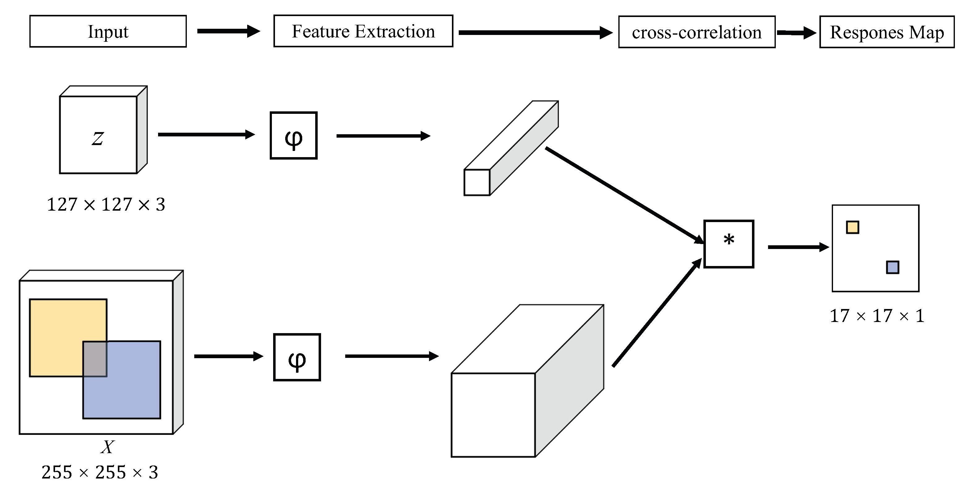
Figure 1. The network framework of SiamFC, where ∗ represents the cross-correlation operation.
Systems 11 00434 g001
Figure 2. Examples of success scenarios for cropping strategies.
Systems 11 00434 g002
Figure 3. Examples of failure scenarios for cropping strategies.
Systems 11 00434 g003
Figure 4. The effect of increasing the target’s scale on Siamese networks.
Systems 11 00434 g004
Figure 5. Demonstration of the effect on the tracker as the target scale increases.
Systems 11 00434 g005
Figure 6. The general framework of our proposed method.
Systems 11 00434 g006
Figure 7. Architecture of multi-scale feature fusion network.
Systems 11 00434 g007
Figure 8. Visualization of feature maps at different levels.
Systems 11 00434 g008
Figure 9. Schematic diagram of the process of 3D Max Filtering.
Systems 11 00434 g009
Figure 10. Schematic diagram of label design.
Systems 11 00434 g010
Figure 11. Examples of video dataset training sample pairs.
Systems 11 00434 g011
Figure 12. Examples of image dataset training sample pairs.
Systems 11 00434 g012
Figure 13. Examples of data augmentation operations.
Systems 11 00434 g013
Figure 14. Example of IoU calculation method, where A represents the ground truth bounding box of the target and B represents the bounding box predicted by the algorithm.
Systems 11 00434 g014
Figure 15. Comparison results for OTB2015 benchmark.
Systems 11 00434 g015
Figure 16. Comparison results for different attributes with respect to VOT2016.
Systems 11 00434 g016
Figure 17. Performance comparison in relation to the VOT2018 dataset.
Systems 11 00434 g017
Figure 18. Demonstration of actual effect.
Systems 11 00434 g018
Table 1. Ablation experiments of our designed method.
NumberBaselineMulti-Scale Feature FusionEllipse Label3D Max FilteringEAOA
1 32.960.1
2 40 . 5 7.6 % 61 . 8 1.7 %
3 41 . 9 9.0 % 61 . 9 1.8 %
4 50 . 2 17.3 % 63 . 3 3.2 %
Table 2. Comparison of multiple trackers applied to VOT2016.
Tracker NameAccuracy ↑Robustness ↓EAO ↑
Ours0.6330.1310.502
SiamDWrpn [13]0.5740.2660.376
CCOT [39]0.5410.2380.331
TCNN [40]0.5550.2680.324
SiamDWfc [13]0.5350.3030.303
SiamBAN [22]0.6320.3960.303
Staple [41]0.5470.3780.295
SiamRN [42]0.5500.3820.277
MDNet [43]0.5420.3370.257
ANT [44]0.4830.5130.203
FPSiamRPN [27]0.609-0.354
Table 3. Performance comparison in relation to GOT10K.
Evaluation MetricsSiamCAR [21]SiamRPN++ [11]SiamBAN [22]DiMP [48]SiamTPN [49]Ours
SR 0 . 5 67.061.564.671.768.672.8
SR 0 . 75 41.532.940.449.344.259.7
AO56.951.754.561.157.664.9
Speed (FPS)513545254060
Table 4. Comparison of tracking speed, the number of parameters in a model, and FLOPs.
TrackersTracking Speed (FPS)No. of Parameters (M)FLOPs (G)GOT10k (AO)OTB100(P)
SiamBAN [22]23.7159.9348.84-91.0
SiamGAT [50]41.9914.2317.2862.791.6
SiamFC++ [20]45.2713.8918.0359.589.6
SiamRPN++ [11]5.1753.9548.9251.791.5
SiamDW [13]52.582.4612.9042.989.2
DiMP-50 [48]30.6743.1010.3561.188.8
SiamRN [42]6.5156.56116.87-93.1
Ours45.0259.7759.3464.991.2
Disclaimer/Publisher’s Note: The statements, opinions and data contained in all publications are solely those of the individual author(s) and contributor(s) and not of MDPI and/or the editor(s). MDPI and/or the editor(s) disclaim responsibility for any injury to people or property resulting from any ideas, methods, instructions or products referred to in the content.