Article

Joint Optimization of Preventive Maintenance and Spare Parts Ordering Considering Imperfect Detection

School of Management Science and Engineering, Anhui University of Technology, Ma’anshan 243002, China
*
Author to whom correspondence should be addressed.
Systems 2023, 11(9), 445; https://doi.org/10.3390/systems11090445
Submission received: 6 July 2023 / Revised: 17 August 2023 / Accepted: 25 August 2023 / Published: 28 August 2023
(This article belongs to the Section Systems Engineering)

Abstract

:
The optimization of preventive maintenance and spare part ordering strategies for modern production equipment is of utmost importance, given its substantial influence on the reliability of equipment systems. Furthermore, the optimization problem discussed here has a direct impact on the reduction of maintenance expenses, thus making it a significant area of research. The optimization of preventive maintenance and spare parts ordering techniques for contemporary industrial equipment, which is a massive and complex system, faces substantial obstacles notwithstanding prior research efforts in the subject. Prior studies have typically assumed a fixed lead time for spare parts ordering, often leading to discrepancies with actual practice. When faced with a critical component failure, such as rolling bearings, it is not advisable for the decision maker to strictly adhere to the ordering strategy. Therefore, this paper presents a novel approach to the maintenance management method, which optimizes preventive maintenance and spare parts ordering strategies using a dynamic early warning period model based on different equipment states. The model incorporates two maintenance approaches, namely normal ordering and emergency ordering, and the equipment will adopt the corresponding maintenance method according to its state. Furthermore, the model takes imperfect detection of equipment states into account since equipment monitoring is not always accurate. Numerical experiments were conducted using rolling bearings, which are a crucial component in typical mechanical equipment, as a case study. The findings indicate that the improved model exhibits a unit time cost of 1.3021, whereas the original model has a unit time cost of 1.3611. Consequently, the new model effectively reduces the maintenance cost. This new method can better resolve the coordination challenge between preventive maintenance and spare parts ordering for equipment, the enhancing of equipment system reliability, and reduce maintenance expenses. In summary, the text presents a significant contribution in the form of a proposed preventive maintenance model that offers increased flexibility, aiming to effectively reduce maintenance costs.

1. Introduction

In modern manufacturing systems, equipment experiences a continuous decline as a result of numerous internal and external factors. If timely maintenance of the equipment is not carried out prior to its failure, it will inevitably result in substantial financial losses and pose safety hazards. Preventive maintenance is a widely used and more flexible maintenance method than corrective maintenance, especially in the face of increasingly complex, sophisticated, and integrated production equipment [1,2]. Different types of preventive maintenance, such as time-based [3], condition-based [4,5,6], or reliability-centered maintenance [7,8], can be implemented depending on specific needs and problems. Compared to other maintenance methods, preventive maintenance offers many advantages, such as enhanced equipment uptime, decreased maintenance expenses, and heightened safety. High reliability and safety are essential for maintaining production efficiency, cost-effectiveness, and long-term business sustainability. This paper aims to address these challenges by developing an innovative and efficient joint preventive maintenance and spare parts ordering strategy.
The development of maintenance operations generates a need for replacement components, consequently impacting the advancement of maintenance [9,10]. Thus, equipment maintenance presents a comprehensive decision-making problem that requires clear coordination between preventive maintenance strategies and spare parts inventory management. Relevant scholars have conducted research on the joint decision-making of preventive maintenance and spare parts. This research can be categorized into three distinct research directions. The first direction focuses on optimizing maintenance decisions and the initial configuration of repairable spare parts [11]. The second direction is concerned with the optimization of maintenance plans and non-repairable spare part ordering strategies [12,13]. The last direction examines imperfect maintenance under the joint decision of maintenance and spare parts [14]. In this paper, we assume that spare parts are non-repairable and address the joint decision-making problem of equipment maintenance and spare parts ordering based on delay time theory. Specifically, our study aims to analyze a delay time model for equipment maintenance and spare parts ordering in order to optimize joint decisions.
The delay time model categorizes the process of equipment deterioration into three distinct states, normal, defective, and failure, with the elapsed time from defect to failure being called the delay time [15,16]. This model has been extensively studied in many academic works, including Christer and Redmond [17,18], as well as Bark and Christer [19]. Wang reviewed the research progress of the delayed time maintenance model from 1999 to 2012 [20], providing a comprehensive summary of the work done in this area which includes important achievements and limitations. In recent years, there has been significant progress in the development and expansion of the delay time model [21]. These advancements have led to the discovery of novel applications in various contexts.
During equipment operation, the system states can be detected, and preventive maintenance measures can be taken based on the current defect state. However, many current studies have focused on the premise of perfect detection, where the actual state of the system can be accurately identified. In reality, detection in complex environments will inevitably produce errors, such as human error and equipment detection error, which can result in inaccurate detection results or imperfect detection [22]. Imperfect detection is a common phenomenon that affects the reliability of equipment maintenance decisions. The impact of imperfect detection on maintenance decision-making has been extensively studied by scholars who have proposed various models and methods to solve this problem. For example, some scholars have developed Bayesian approaches to estimate system failure probabilities using imperfect detection data [23,24], while others have proposed fuzzy logic-based techniques to account for uncertainty and imprecision in detection processes [25]. Therefore, in order to enhance the efficacy of maintenance strategies, it is crucial to take into account the presence of imperfect detection in equipment maintenance and spare parts ordering strategies.
Detection errors can be categorized into two distinct types: false positive detection errors and false negative detection errors [26,27,28]. False-positive detection errors occur when the test result erroneously indicates a fault state, despite the true state of the system being normal. Conversely, false-negative detection errors manifest when the test outcome indicates normalcy, despite the actual state of the system being a fault state. Imperfect detection plays a crucial role in influencing decisions related to equipment maintenance. Scholars have conducted relevant studies considering imperfect detection, such as Liu et al. [29], who investigated the track maintenance optimization model under false negatives in railway quality control system detection. Furthermore, recent studies have shown that a two-phase inspection strategy can reduce maintenance costs [30,31,32] although most existing strategies for two-phase detection assume perfect detection. In this paper, we propose a two-phase detection strategy to optimize maintenance decisions for an imperfect detection system undergoing three degradation states. Our approach aims to improve the efficiency and stability of the system by accounting for the effects of imperfect detection. Specifically, our study makes a significant contribution by applying a two-phase inspection strategy to optimize maintenance decisions, thus providing a more effective and realistic solution to the problem of joint decision-making between equipment maintenance and spare parts ordering in the presence of imperfect detection.
In addition, most studies on the joint decision-making of preventive maintenance and spare parts ordering assume a fixed lead time for ordering [33,34], but in practice, more flexible ordering strategies are often adopted when spare parts need to be ordered. For instance, when equipment failure occurs and results in significant economic losses, faster shipping methods may be used, even if this incurs additional transportation costs. To address these practical concerns, we propose an emergency ordering operation on top of the fixed lead time assumption. Specifically, a normal order is placed when equipment is detected to be in a defective state and when spare parts are not available, an emergency order is placed when equipment fails. By incorporating this particular feature into the spare part ordering strategy, manufacturers can enhance their ability to promptly and efficiently address equipment failures, thereby minimizing potential financial setbacks. Compared to other research, our approach offers a more effective and innovative solution to the problem of joint decision-making between equipment maintenance and spare part ordering. Furthermore, this study addresses some of the gaps in the existing literature and contributes to a better understanding of the challenges faced by manufacturers in practice.
This paper introduces a comprehensive decision optimization problem that employs a two-phase inspection strategy and spare parts ordering, taking into consideration the presence of imperfect detection. Specifically, we consider false-negative detection as the primary form of imperfection, and once the equipment is detected to be in a defective state, preventive replacement is conducted based on the current stock of spare parts. Our goal is to determine the optimal duration of the phase I and phase II testing cycle, spare parts ordering time, and emergency ordering lead time, assuming an unlimited time domain in order to minimize the cost per unit time. By incorporating the emergency ordering lead time as a decision variable, we can respond more effectively to unexpected equipment failures, reducing the risk of economic losses. To demonstrate the advantages of our proposed model, we compare it with the fixed lead time detection model. Our approach offers a more rigorous and logical solution to the joint decision-making problem of equipment maintenance and spare parts ordering, highlighting the benefits of incorporating an imperfect detection mechanism and flexible ordering strategy.
The article is organized as follows. Section 2 presents a detailed description of preventive maintenance issues that take into account imperfect detection and spare parts ordering. In Section 3, we adopt the renewal reward theorem to construct a joint optimization model for two-phase detection and spare parts ordering. The goal of this model is to minimize the expected cost per unit time of equipment. In Section 4, a case analysis is presented, where the proposed model is solved using the particle swarm optimization algorithm. The obtained results are then compared with those of the fixed lead time model. Finally, Section 5 presents our conclusions and outlines several future research directions. The contribution of this paper is to propose a new model that is more flexible than the traditional model and can effectively reduce maintenance costs.

2. Problem Description

The degradation of the equipment from the new state to the failure state goes through the normal operation phase and then the defect phase, which are independent of each other and follow a certain distribution. A two-phase detection strategy is adopted for the detection of equipment: the first phase of detection is performed at time  T , and then the equipment is detected every regular interval  t . The detection is imperfect, according to the probability of false negative events, and spare parts are ordered at a discrete moment. Corresponding maintenance measures are taken according to the recognition states of the equipment at this moment and the spare parts inventory states when the equipment is maintained, as shown in Figure 1.

2.1. Maintenance Model Assumptions

  • The equipment is a single component system and is not repairable.
  • There is only one failure mode of the equipment, and the time domain is infinite.
  • A two-phase inspection strategy is adopted, the first stage is executed at the  T  moment, and then the equipment is tested in cycles  t   ( t < T ) , and the cost of each test is  C d . The detection consumption time is much smaller than the detection cycle and is negligible.
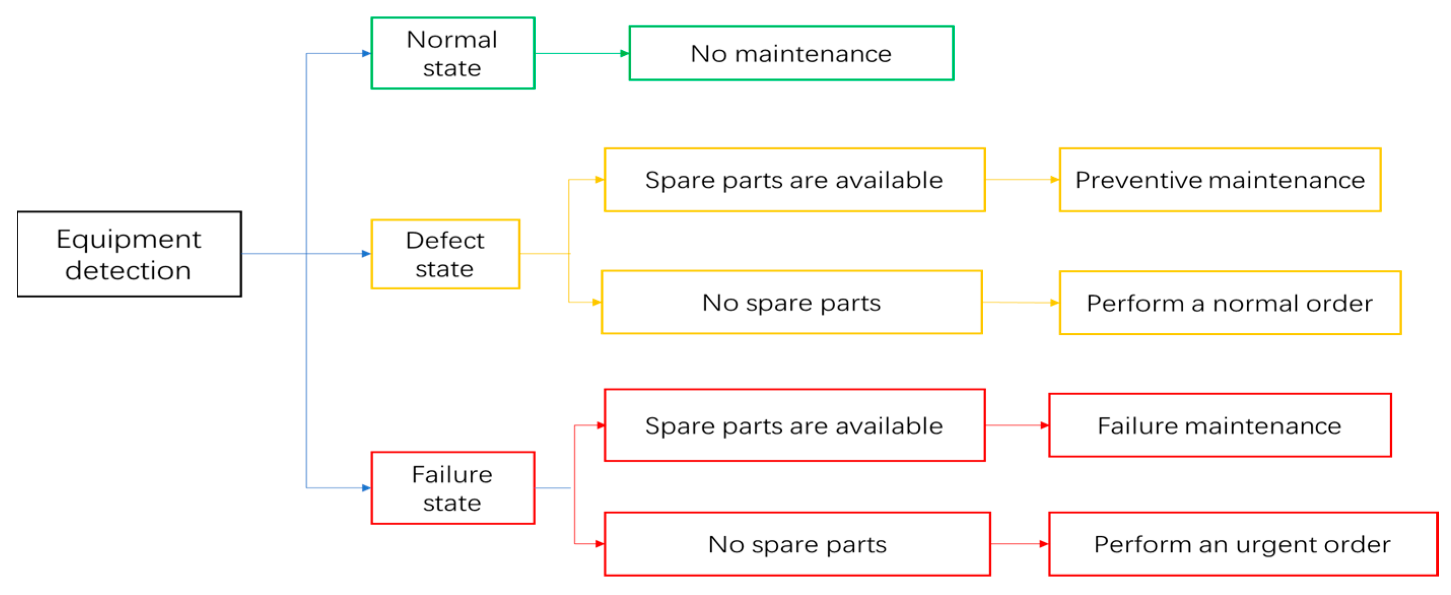
  • The detection is imperfect, and a false negative event occurs according to the probability of detection, that is, the equipment is actually in a defective state, and the detection is judged by probability  p   ( 0 < p < 1 )  that the equipment is in a normal state.
  • When a defective condition is detected, a preventive maintenance is carried out at cost  C p . Equipment failure will automatically shut down, at this time the fault maintenance is carried out at the cost  C f .
  • A delayed ordering strategy is adopted, i.e., spare parts are ordered at the ε (ε > 0) moment, with a lead time of  L  for normal orders and  L s  for urgent orders, and an order quantity of 1. There may be 3 different states of spare parts when the equipment is maintenanced: a spare parts state of 0 indicates that the spare parts have not been ordered; A spare part states of 1 indicates that it has been ordered and has not yet entered the inventory; A states of 2 for a spare part indicates that the part is currently being stored and is available in inventory.
  • The penalty cost per unit time of waiting for spare parts for preventive and faulty maintenance of equipment is  C w P  and  C w f , and  C w P  <  C w f , respectively. The unit of time holding cost of spare parts in inventory is  C h . The cost of equipment renewal  C p  or  C f  includes the cost of ordering spare parts, own costs, and maintenance personnel.

2.2. Symbol Description

The symbols and meanings used in the model of this paper are shown in Table 1. And Table 2 shows the model parameters

3. Maintenance Cost Models

The optimization model proposed in this paper aims to determine the optimal first stage detection time  T , the second stage detection cycle  t , spare parts order time ε, and emergency order lead time  L s  as the goal, so as to achieve the minimum expected cost per unit time. Determine all possible scenarios based on how the equipment is maintenanced at the time of the implementation of the detection strategy and the state of the spare parts, and then obtain the probability of occurrence, expected cost, and expected length of each maintenance event, and then obtain the total expected cost and expected length.

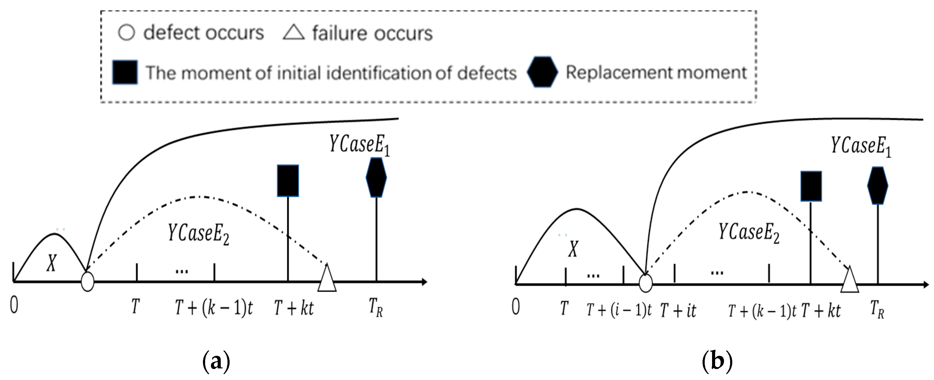
3.1. Renewal Scenarios 1 and 2

The first type of maintenance process is when  T + k t  detects that the equipment is in a defective state and the spare parts state is 0 or 1.
When the states of spare parts is 0, at this time ε   T + k t , a normal order should be made immediately, then wait for the delivery time  T R = T + k t + L , and then maintenance the equipment. When the spare parts state is1, at this time  ε T + k t < ε + L , waiting for the delivery time is  T R = ε + L  before performing maintenance on the equipment. Considering that false negative events may occur during the detection process, it is divided into two situations according to the moment of the equipment defect point: one is that the defect occurs within [0, T], and the defect is detected at the time of  T + k t , when k = 0, it means that no false negative event has occurred, and when k ≠ 0, k false negative events have occurred. Second, the defect occurs in  T + i 1 t , T + i t ,  and a total of (k-i) false negative events occur, which are represented by Figure 2a,b. In addition,  C a s e E 1  indicates that the equipment is in a defective state at the  T R  moment, and  C a s e E 2  indicates that the equipment is in a faulty state at this time, and so the fault maintenance is carried out at the  T R  moment.
As shown in the  C a s e E 1  in Figure 2a,b, the probability of a piece of equipment having a preventive maintenance at  T R  moment is as follows:
P 1 , a E 1 T R = 0 T T R x p k 1 p f X x f Y y d y d x
P 1 , b E 1 T R = i = 1 k T + i 1 t T + i t T R x p k i 1 p f X x f Y y d y d x
As shown in the  C a s e E 2  in Figure 2a,b, the probability of a piece of equipment failing to maintenance at  T R  moment is:
P 1 , a E 2 T R = 0 T T + k t x T R x p k 1 p f X x f Y y d y d x
P 1 , b E 2 T R = i = 1 k T + i 1 t T + i t T + k t x T R x p k i 1 p f X x f Y y d y d x
Combined with the probability of preventive renewal in Equations (1) and (2), the expected cost of preventive maintenance at the  T R  moment  E C 1 T , t , ε , L s  and the expected length  E L 1 T , t , ε , L s  are:
E C 1 T , t , ε , L s = k = 0 k + 1 C d + C p + T R T k t C w p · P 1 , a E 1 T R + k = 1 k + 1 C d + C p + T R T k t C w p · P 1 , b E 1 T R
E L 1 T , t , ε , L s = k = 0 T R · P 1 , a E 1 T R + k = 1 T R · P 1 , b E 1 T R
Combined with the probability of failure maintenance in Equations (3) and (4), the expected cost of failure maintenance of the equipment at the  T R  time    E C 2 T , t , ε , L s  and the expected length  E L 2 T , t , ε , L s  are:
E C 2 T , t , ε , L s = k = 0 k + 1 C d + C f + T f T k t C w p + T R T f C w f · P 1 , a E 1 T R + k = 1 k + 1 C d + C f + T f T k t C w p + T R T f C w f · P 1 , b E 1 T R
E L 2 T , t , ε , L s = k = 0 T R · P 1 , a E 2 T R + k = 1 T R · P 1 , b E 2 T R

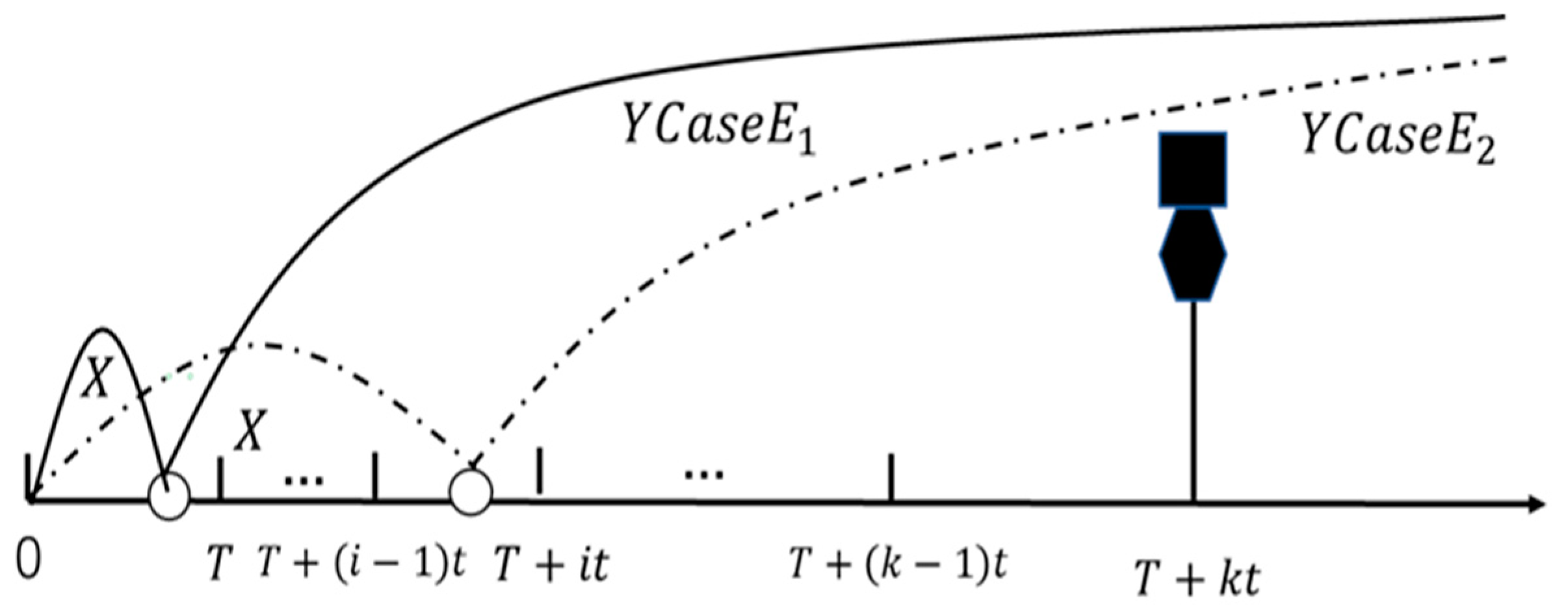
3.2. Renewal Scenario 3

The third type of maintenance process is  T + k t  detection at all times to identify the equipment as defective and spare parts as two. There are two cases depending on the moment the defect is happen, as show in Figure 3. And since the spare parts state is 2, preventive maintenance is taken immediately at the  T + k t  moment.
As shown in Figure 3 Case  E 1  and Case  E 2 , the probability of preventive maintenance of the equipment at the time of  T + k t  is:
P 2 E 1 T R = 0 T T + k t x p k 1 p f X x f Y y d y d x
P 2 E 2 T R = i = 1 k T + i 1 t T + i t T + k t x p k i 1 p f X x f Y y d y d x
According to Equations (9) and (10), the expected cost  E C 3 T , t , ε , L s  and expected length  E L 3 T , t , ε , L s  of the equipment at the  T + k t  moment is obtained as follows:
E C 3 T , t , ε , L s = k = 0 k + 1 C d + C p + T + k t ε L C h · P 2 E 1 T R + k = 1 k + 1 C d + C p + T + k t ε L C h · P 2 E 2 T R
E L 3 T , t , ε , L s = k = 0 T + k t · P 2 E 1 T R + k = 1 T + k t · P 2 E 2 T R

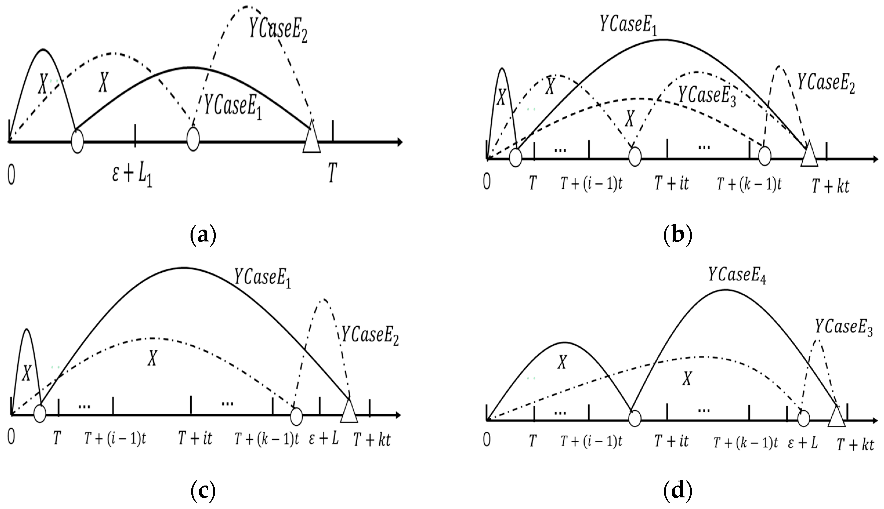
3.3. Renewal Scenario 4

The fourth type of equipment maintenance scenario is when the equipment fails and stops at the  T f  moment and the spare parts state is zero. Figure 4 C a s e E 1  indicates that the equipment defect occurred before the first inspection time, because the spare part state was zero at this time, so the equipment failure time meets  T f < m i n T , ε . A  C a s e E 2  of Figure 4a indicates that the equipment failed before the defect was detected, meeting  T f < m i n T + k t , ε . Figure 4b indicates that the defective moment of the equipment is  T + k 1 t , m i n T + k t , t , and since the spare part states is zero, it satisfies  T f < m i n T + k t , ε . Figure 4c indicates that the defective moment of the equipment is  T + i 1 t , T + i t , which also satisfies  T f < m i n T + k t , ε .
As shown in Figure 4a–c, the probability of the maintenance failure of the equipment in various different situations is as follows:
P 3 , a E 1 T R = 0 m i n T , ε 0 min T , ε x f X x f Y y d y d x
P 3 , a E 2 T R = 0 T T + k 1 t x min T + k t , ε x p k f X x f Y y d y d x
P 3 , b T R = T + k 1 t m i n T + k t , ε 0 min T + k t , ε x f X x f Y y d y d x
P 3 , c T R = i = 1 k 1 T + i 1 t T + i t T + k 1 t x min T + k t , ε x p k i f X x f Y y d y d x
According to Equations (13)–(16), the expected cost of the equipment under maintenance scenario 4    E C 4 T , t , ε , L s  and the expected length  E L 4 T , t , ε , L s :
E C 4 T , t , ε , L s = C f + L s C w f · P 3 , a E 1 T R + k = 1 k C d + C f + L s C w f · P 3 , a E 2 T R + P 3 , b E 1 T R + k = 2 k C d + C f + L s C w f · P 3 , c E 1 T R
E L 4 T , t , ε , L s = T f + L s · P 3 , a E 1 T R + k = 1 T f + L s · P 3 , a E 2 T R + P 3 , b E 1 T R + k = 2 T f + L s · P 3 , c E 1 T R

3.4. Renewal Scenario 5

The fifth maintenance scenario is when the equipment fails and stops at the  T f  moment and the spare parts state is one, at which point the  ε < T f < ε + L s  is established. According to the time of equipment defect and the fault occurrence interval, it can be divided into five situations, if the equipment fails within [0, T], there is  ε < T f < m i n T , ε + L s , as shown in Figure 5a; If the fault occurs in  T + k 1 t , T + k t , then there is  T + k 1 t < T f < m i n T + k t , ε + L s , as shown in Figure 5b.
Figure 5a considers two cases where the equipment fails within  0 , T  and the fault maintenance is performed at the  ε + L s  moment, and their failure maintenan probabilities are:
P 4 , a E 1 T R = 0 ε ε x min T , ε + L s x f X x f Y y d y d x
P 4 , a E 2 T R = ε m i n T , ε + L s 0 min T , ε + L s x f X x f Y y d y d x
Figure 5b considers three cases where the equipment fails in  T + k 1 t , T + k t , and the fault maintenance is performed at the  ε + L s  moment. Their failure maintenance probabilities are:
P 4 , b E 1 T R = 0 T T + k 1 t x min T + k t , ε + L s x p k f X x f Y y d y d x
P 4 , b E 2 T R = T + k 1 t m i n T + k t , ε + L s 0 min T + k t , ε + L s x f X x f Y y d y d x
P 4 , b E 3 T R = i = 1 k 1 T + i 1 t T + i t T + k 1 t x min T + k t , ε + L s x p k i f X x f Y y d y d x
According to Equations (19)–(23), the expected cost of the equipment in maintenance scenario 5  E C 5 T , t , ε , L s  and the expected length  E L 5 T , t , ε , L s  are as follows:
E C 5 T , t , ε , L s = C f + ε + L s T f C w f · P 4 , a E 1 T R + P 4 , a E 2 T R + k = 1 k C d + C f + ε + L s T f C w f · P 4 , b E 1 T R + P 4 , b E 2 T R + k = 2 k C d + C f + ε + L s T f C w f · P 4 , b E 3 T R
E L 5 T , t , ε , L s = k = 1 ε + L s · P 4 , b E 1 T R + P 4 , b E 2 T R + k = 2 ε + L s · P 4 , b E 3 T R + ε + L s · P 4 , a E 1 T R + P 4 , a E 2 T R

3.5. Renewal Scenario 6

The sixth maintenance scenario is when the equipment fails at the  T f  time and the spare parts state is 2, indicating that the spare parts are in stock before the failure, and the lead time is   L ,  meeting the  ε + L T f . Depending on the range in which the equipment failure occurs, consider the following situations as shown in Figure 6.
Figure 6a considers that the equipment failure occurs within  0 , T , and is divided into two cases according to the relationship between the time of equipment defect and the size of  ε + L . Their maintenance probability is calculated as follows:
P 5 , a E 1 T R = 0 ε + L ε + L x T x f X x f Y y d y d x
P 5 , a E 2 T R = ε + L T ε + L x T x f X x f Y y d y d x
Figure 6b considers that the equipment failure occurs in  T + k 1 t , T + k t , which is divided into three situations according to the different defect moments of the equipment. Their maintenance probability is as follows:
P 5 , b E 1 T R = 0 T T + k 1 t x T + k t x p k f X x f Y y d y d x
P 5 , b E 2 T R = T + k 1 t T + k t 0 T + k t x f X x f Y y d y d x
P 5 , b E 3 T R = i = 1 k 1 T + i 1 t T + i t T + k 1 t x T + k t x p k i f X x f Y y d y d x
Figure 6c considers that the equipment failure occurs in  T + k 1 t , ε + L . It is divided into two situations according to the different defect moments of the equipment. Their maintenance probability is as follows:
P 5 , c E 1 T R = 0 T ε + L x T + k t x p k f X x f Y y d y d x
P 5 , c E 2 T R = T + k 1 t ε + L ε + L x T + k t x f X x f Y y d y d x
Figure 6d considers that the equipment failure occurs in  ε + L , T + kt , which is didvided into two situations according to the different defect moments of the equipment. Their maintenance probability is as follows:
P 5 , d E 3 T R = ε + L T + k t 0 T + k t x f X x f Y y d y d x
P 5 , d E 4 T R = i = 1 k 1 T + i 1 t T + i t ε + L x T + k t x p k i f X x f Y y d y d x
According to Equations (26)–(34), the expected cost of updating scenario 6  E C 6 T , t , ε , L s  and the expected length  E L 6 T , t , ε , L s  are:
E C 6 T , t , ε , L s = C f + T f ε L C h · P 5 , a E 1 T R + P 5 , a E 2 T R + k = 1 k C d + C f + T f ε L C h · P 5 , b E 1 T R + P 5 , b E 2 T R + P 5 , c E 1 T R + P 5 , c E 2 T R + P 5 , d E 3 T R + k = 2 k C d + C f + T f ε L C h · P 5 , d E 3 T R + P 5 , d E 4 T R
E L 6 T , t , ε , L s = T f · P 5 , a E 1 T R + P 5 , a E 2 T R + k = 1 T f · P 5 , b E 1 T R + P 5 , b E 2 T R + P 5 , c E 1 T R + P 5 , c E 2 T R + P 5 , d E 3 T R + k = 1 T f · P 5 , b E 3 T R + P 5 , d E 4 T R

3.6. Joint Decision Model

According to the expected cost and expected length of the equipment in all cases, a two-phase inspection and spare parts ordering strategy joint decision model with the minimum expected cost  C T , t , ε , L s  per unit time is constructed as follows:
C T , t , ε , L s = E C T , t , ε , L s E L T , t , ε , L s = k = 1 6 E C k T , t , ε , L s k = 1 6 E L k T , t , ε , L s
Due to the wide application of the Weibull distribution in the field of reliability analysis, this paper uses the Weibull distribution method to describe the degradation process of equipment during a normal operation and defect phase. The probability density funtion of the Weibull distribution is as follows:
f x , λ , k = k λ x λ k 1 e x λ k       x 0

4. Numerical Examples

A large number of critical single components are found in industrial production equipment, such as small motors, battery packs, rolling bearings, etc. This article uses rolling bearings as an example to verify the validity of this model in industrial production.

4.1. Model Solving Using Particle Swarm Optimization Algorithm

First, we give a description of the nature of this optimization problem. As can be seen from the model, this is a nonlinear optimization problem. Specifically, it is an integer programming problem with four decision variables. The methods to solve such problem are not unique, there are currently common heuristic algorithms and some gradient descent algorithms, and NLopt also offers a range of nonlinear optimization algorithms.
In this paper, the particle swarm optimization algorithm is used to solve the joint decision-making model, and the pseudocode for model solving is given. Here is a brief introduction to the particle swarm optimization algorithm and the selection of parameters in the algorithm is described in detail. The particle swarm optimization algorithm is a heuristic algorithm, proposed by American scholars Eberhart and Kennedy in 1995, which continuously maintains the individual suboptimal solution by simulating the process of bird foraging in nature. It is worth noting that particles are limited by position and speed during iteration. The reason for implementing a position limit is that the decision variables in this model have a value range from zero to infinity. Taking into account the practical context, the four decision variables in this paper—the first stage detection time  T , the second stage detection time  t , spare parts ordering time  ε , and the urgent order lead time  L s  are all constrained to positive integers.
In Table 3 the symbol  N  is used to indicate the particle swarm size. Smaller population size is easy to fall into local optimum and larger scales can improve convergence but increase the amount of calculation. Since the objective function is a bit complex, 100 is enough here. There are a total of four decision variables in the model, so here the particle dimension  D  is set to four. If the number of iterations  K  is too small, the solution will be unstable, too large will be very time-consuming, there is no need, here  K  is set to 200.  c 1  and  c 2  are called learning factors, and it is acceptable to choose numbers between 0–4, and in general,  c 1  and  c 2  take the same number (not mandatory).  W m a x  and  W m i n  are called inertial weights, and the value of  W    is linearly reduced with the increase in the number of iterations, so that the algorithm has strong global convergence ability in the early stage and strong local convergence ability in the later stage. Any number between 0.4–2 is acceptable.  V m a x  and  V m i n  are the speed limits of particles, there are no specific requirements, and  V m a x  is generally set to the absolute value of  V m i n .
A description of the parameter in Equation (38): where  λ  is the scale parameter and k is the shape parameter. The normal stage and defect stage parameters of the equipment are set to:  λ 1  = 17.24,  k 1  = 1.47;  λ 2  = 6.25,  k 2  = 1.14. The other parameters in the model are shown in Table 2, where the time parameter unit is days, and the cost parameter unit is 10,000. Here, we need to pay attention when giving the parameters of the Weibull distribution: since the random variable  x  in the probability density function represents time, and  λ  in the Weibull distribution is the proportional parameter, the larger the proportional parameter, the curve of the probability density function will be shifted to the right. That is, that it has the characteristics of a right-biased distribution. The defect phase of the equipment occurs after the normal phase, and when the equipment runs for a considerable period of time (without failure), the probability density corresponding to the normal phase should be greater than the probability density of the defect stage. This requires  λ 1  >  λ 2  to be established, and this model describes the degradation process of the equipment, so the shape parameter k satisfies k > 1. When actually using this model, it is necessary to select appropriate parameter values according to the different application scenarios. Algorithm 1 shows the process of the PSO algorithm.
Algorithm 1. Joint decision model algorithm process.
Step 1: Initialization process
FOR each particle  i
 FOR each dimension  d
  Initialize the position  x i d     and   velocity   v i d  randomly of each particle  i ;
  Plug in the initial solution to Formula (37) to obtain the personal best position  p b e s t i d  of each particle
  Initialize the population’s best position value  g b e s t   =   m i n ( p b e s t i d )
 END FOR
END FOR
Step 2: Iterative optimization process.
Iteration  K = 1
DO
  FOR each particle  i
   Calculate fitness value
    personal best position and value
    IF objective function  C T , t , ε , L s  for each  x i d     <     p b e s t i d
     p b e s t i d  =  C T , t , ε , L s  for each  x i d
     p b e s t i d =   x i d  
    END IF
 END FOR
 Choose the particle having the best fitness value as the  p g b e s t i d
 FOR each particle  i  
  FOR each dimension  d  
  Calculate the dynamic inertia weight value.
   w   =   W m a x     W m a x W m i n i / K ;  
  Maintenance position and velocity values.
   v i d =   w v i d + c 1 r a n d p b e s t i d x i d + c 2   r a n d p g b e s t i d x i d ;
   x i d   =   x i d + v i d ;  
  Boundary condition handling.
    i f ( v i d   >   V m a x )   | |   ( v i d   <   V m i n )
    v i d   =   r a n d     V m a x V m i n   +   V m i n ;
  END FOR
 END FOR
  % Use  g b  to record the historical global best solution.
   g b   = p g b e s t i d ;
   K   =   K + 1  
 %When the number of iterations reaches  K , the iteration process ends. The best solution obtained in each iteration will be obtained, and the largest  g b  is the global best solution:  C T * , t * , ε * , L s *  

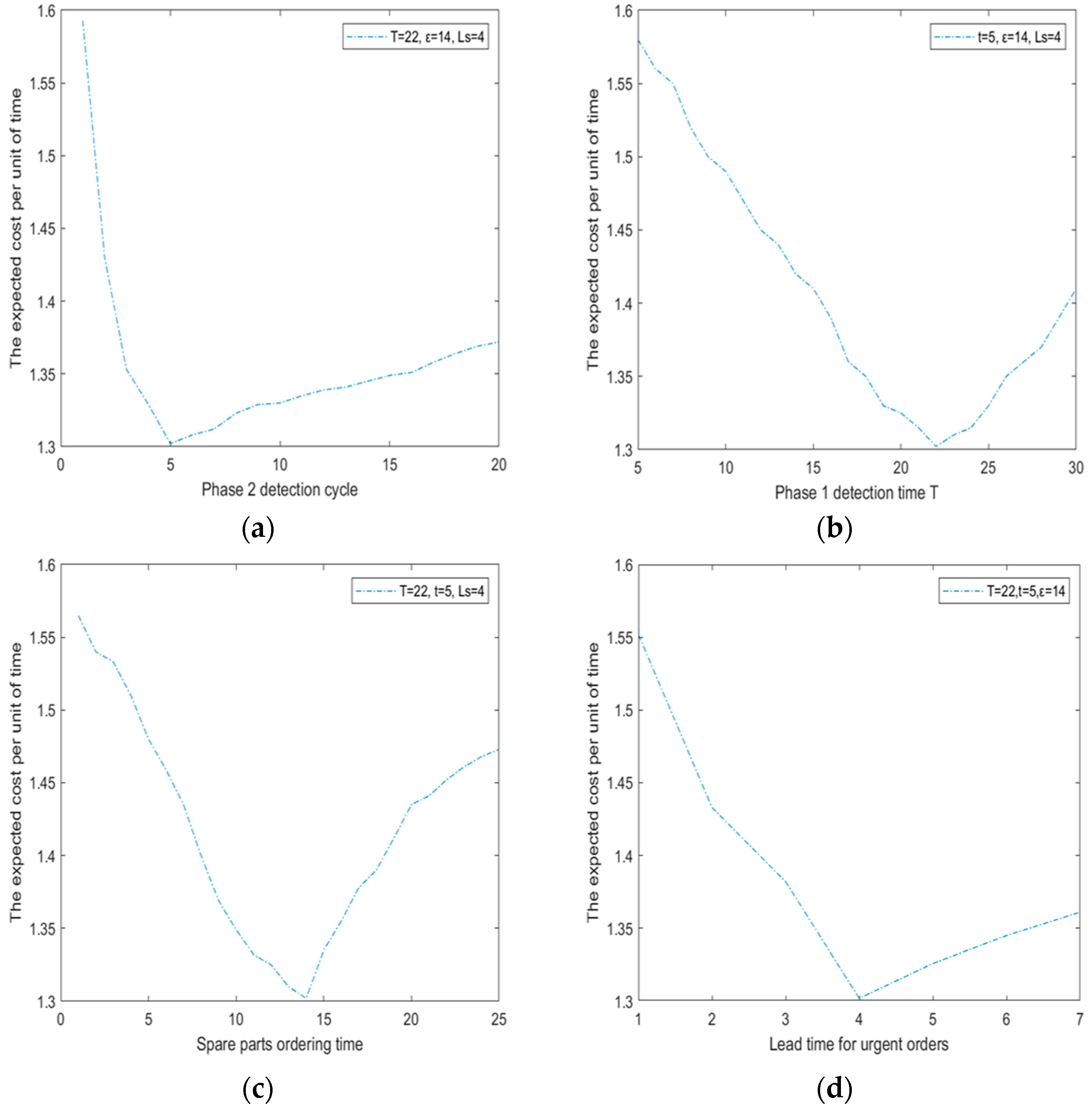
4.2. Sensitivity Analysis

According to the model parameters in Table 2, the algorithm parameters in Table 3 and the equipment degradation process distribution parameters, the PSO algorithm is used to solve the model, and the suboptimal solution is as follows. The detection time of the first stage,  T *  = 22,  t *  = 5,  ε *  = 14,  L s *  = 4, and the minimum unit time cost is  C T * , t * , ε * , L s *  = 1.3021 under the optimal combination strategy. Then, the decision variables are set to be optimized in the model  L s  fixed value, that is,  L s  =    L , indicating that the model adopts a fixed lead time, and the suboptimal solution can be obtained by using the PSO algorithm again,  T *  = 20,  t *  = 3,  ε *  = 13, and the minimum unit time cost is  C T * , t * , ε *  = 1.3611. From 1.3021 < 1.3611. The detection strategy proposed in this paper is better than the detection strategy with a fixed lead time. Since the objective function contains four decision variables in order to explore the change of the minimum unit time cost with any decision variable, it is necessary to fix any three of the decision variables, and plot the change curve of the minimum unit time cost C with the first stage detection time T, the second stage detection cycle t, spare parts order time ε, and emergency order lead time  L s , as shown in Figure 7
As shown in Figure 7a, C decreases first and then increases with the increase in the first stage detection time T, which is also intuitively predicted. Because the first stage of testing time T is very small, the number of times the equipment needs to be tested will obviously increase, the required testing cost will be very large. When T gradually increases, the number of times the equipment needs to be tested will naturally decrease, here the detection refers to the equipment from the beginning of work to the first detection of defects (or failure shutdown) during the inspection. However, when T increases to a critical value, C does not decrease anymore, because when T is very large, it is very likely that the equipment will enter a defect state and fail before the first detection, and this result is discussed in more detail here. The first case is that the equipment enters the defect state before T but does not fail due to the influence of imperfect detection. A false negative event occurs at the T moment, so the increase in T leads to a decrease in the probability of the equipment being detected as a defect, which in turn leads to an increase in the cost of fault maintenance, which is manifested as an increase in C. The second case is that the equipment fails before T, which obviously leads to an increase in the cost of failure maintenance, which also manifests itself as an increase in C.
As shown in Figure 7b, C decreases and then increases with the increase in the second stage detection cycle t, which is similar to the explanation of C with the increase in the first stage detection time T first decreases and then increases, when T takes a smaller value, the equipment required for testing costs will increase, when exceeding a certain critical value, because the detection is not perfect, the equipment may fail in the process of waiting for the next test, resulting in a larger fault maintenance cost, manifested as the increase in C.
Figure 7c shows that C first decreases and then increases with the increase in spare parts ordering time ε which is well explained because the spare parts ordering time ε represents premature holding of spare parts, which will lead to an increase in the cost of ownership. If ε is too large, it means that the equipment has failed to order spare parts, which obviously increases the penalty cost of waiting for spare parts. Especially for expensive spare parts and equipment susceptible to environmental influences, the choice of ordering time ε the impact on C will be more obvious.
Figure 7d shows that C decreases first and then increases with the increase in the emergency order lead time  L s , this change is intuitive and a detailed explanation is given below. From  C e = k L L s , it can be seen that the additional cost of emergency ordering is linearly related to  C e   L s , and the  C e  decreases as the  L s  increases, which explains the first half of Figure 6d: Consider an extreme case, when the  L s  is infinitely close to zero, the  C e  at this time will be large, which means that there is a huge cost to make an emergency order at this time. Of course this does not happen in reality because spare part orders always take a certain amount of time to reach inventory. As the  L s  increases, the additional costs required  C e  decrease. However, when the  L s  increases to a critical value, although the  C e  will decrease. The expected cost C per unit time will not decrease again but gradually increase because when the  L s  is larger ( L s < L ), the equipment still has to wait for a long time for spare parts to arrive, that is, the maintenance failure penalty cost is not reduced by much when the emergency order is taken, and an additional cost is to be borne by it, so C does not decrease but instead increases. The change of C with  L s  also shows the rationality of increasing the emergency ordering scheme and that setting the optimal  L s  value can make the model more flexible and in line with the actual situation.
Table 4 shows the suboptimal solution and optimal value of the model when the probability of a false negative event occurrence p takes different values while keeping other parameters unchanged. It can be seen from the table that with the increase in p, the suboptimal solution of the first stage of the detection cycle  T *  and the spare parts ordering time  ε *  gradually increases because the increase in p increases the number of false negative events, resulting in an increase in testing costs. Decision-makers will reduce the cost of testing by increasing the first stage of detection time and increase the spare parts ordering time to reduce the cost of ownership, thereby reducing the expected cost per unit time.
Table 5 shows the sensitivity analysis results of each cost parameter in the model that increases by 30% when it is unchanged. It can be seen that when the detection cost  C d  and the preventive maintenance cost  C p  increase, in order to obtain the minimum detection cost per unit time, the first stage detection time will increase and the detection cycle will decrease accordingly. When the cost of fault maintenance  C f  increases with  C w f , the occurrence of faults can be reduced by increasing the detection frequency, so as to obtain the minimum cost; The increase in the  C h  of holding costs has led decision makers to increase the time it takes to order spare parts to reduce the cost of holding spare parts in inventory. The lead time for emergency orders is only affected by  C w f , because there are only two situations that trigger urgent orders. One is when the equipment is detected to be defective and the spare parts state is zero, and the other is when the equipment fails, and the spare parts state is zero. The purpose of the increased emergency ordering strategy is to reduce the penalty cost of spare parts in both cases. In the first case, although the  C w p  increases, the  L s *  does not change. One of the reasons is that the spare parts are already in stock when the defect is detected, and naturally there is no corresponding  C w p , and the second reason is that  C w p  is a small value relative to  C w f , so it has no effect on  L s * . In the second case, as the  C w f  increases, the  L s *  needs to be reduced to reduce the penalty cost in the event of a failed maintenance. Finally, it can be observed that the expected cost per unit time is not sensitive to  C w p , because the cost of holding spare parts is  C h  <  C w p , so the optimal decision is more inclined to hold spare parts before the equipment detects a defect, which is similar to the explanation of the effect of  C w p  on  L s * . In summary, the optimal decision of equipment maintenance and spare parts ordering is affected by the combination of various parameters, so it is necessary to consider the joint optimization of preventive maintenance decisions for imperfect detection and spare parts ordering.

5. Conclusions

This paper proposes a new joint decision-making model for equipment maintenance and spare parts ordering that is more realistic and effective in dealing with the uncertainties of delivery time and the effects of imperfect detection. By integrating a two-phase inspection methodology and an emergency ordering mechanism, our proposed model offers a heightened level of adaptability and responsiveness in order to optimize decisions regarding preventive maintenance and reduce costs over a given time period. Under the condition of keeping the parameters fixed, the maintenance cost per time obtained by the proposed model is 1.3021, compared to 1.3611 in the original model. By comparison, the improved model can effectively reduce maintenance costs. Our findings emphasize the importance of considering the practical issues encountered in actual production, such as unexpected equipment failures and uncertain delivery times. In future research, we will consider extending the single component system model to systems with several identical components and adding constraints on related resources, such as the availability of spare parts. In general, our approach presents a promising solution for manufacturers seeking to enhance their equipment maintenance strategies and minimize operational expenses.

Author Contributions

Methodology, Y.H.; software, Y.H.; validation, Y.H. and Z.G.; formal analysis, Y.H.; writing—original draft preparation, Y.H.; All authors have read and agreed to the published version of the manuscript.

Funding

This research was funded by the Science Research Project of Anhui Higher Education Institutes (No. 2022AH040050).

Data Availability Statement

Not applicable.

Conflicts of Interest

The authors declare no conflict of interest.

References

  1. Basri, E.I.; Razak, I.H.A.; Ab-Samat, H.; Kamaruddin, S. Preventive maintenance (PM) planning: A review. J. Qual. Maint. Eng. 2017, 23, 114–143. [Google Scholar] [CrossRef]
  2. Aminu Sahabi Abubakar, Z.H.; Aime, C. Nyoungue, Production System Optimisation with a Multi-Level Process Control Tool Integrated into Maintenance and Quality Strategies under Services and Quality Constraints. Eur. J. Sci. Innov. Technol. 2023, 3, 302–320. [Google Scholar]
  3. Syamsundar, A.; Naikan, V.; Wu, S. Estimating maintenance effectiveness of a repairable system under time-based preventive maintenance. Comput. Ind. Eng. 2021, 156, 107278. [Google Scholar] [CrossRef]
  4. Chuang, C.; Ningyun, L.; Bin, J.; Yin, X. Condition-based maintenance optimization for continuously monitored degrading systems under imperfect maintenance actions. J. Syst. Eng. Electron. 2020, 31, 841–851. [Google Scholar] [CrossRef]
  5. Dao, C.D.; Kazemtabrizi, B.; Crabtree, C.J.; Tavner, P.J. Integrated condition-based maintenance modelling and optimisation for offshore wind turbines. Wind Energy 2021, 24, 1180–1198. [Google Scholar] [CrossRef]
  6. Wang, J.; Qiu, Q.; Wang, H.; Lin, C. Optimal condition-based preventive maintenance policy for balanced systems. Reliab. Eng. Syst. Saf. 2021, 211, 107606. [Google Scholar] [CrossRef]
  7. Hussain, Z.; Jan, H. Establishing simulation model for optimizing efficiency of CNC machine using reliability-centered maintenance approach. Int. J. Model. Simul. Sci. Comput. 2019, 10, 1950034. [Google Scholar] [CrossRef]
  8. Palei, S.K.; Das, S.; Chatterjee, S. Reliability-Centered Maintenance of Rapier Dragline for Optimizing Replacement Interval of Dragline Components. Min. Metall. Explor. 2020, 37, 1121–1136. [Google Scholar] [CrossRef]
  9. Kuppulakshmi, V.; Sugapriya, C.; Kavikumar, J.; Nagarajan, D. Fuzzy Inventory Model for Imperfect Items with Price Discount and Penalty Maintenance Cost. Math. Probl. Eng. 2023, 2023, 1246257. [Google Scholar] [CrossRef]
  10. Zhang, J.-X.; Du, D.-B.; Si, X.-S.; Hu, H.-W. Joint optimization of preventive maintenance and inventory management for standby systems with hybrid-deteriorating spare parts. Reliab. Eng. Syst. Saf. 2021, 214, 107686. [Google Scholar] [CrossRef]
  11. de Pater, I.; Mitici, M. Predictive maintenance for multi-component systems of repairables with Remaining-Useful-Life prognostics and a limited stock of spare components. Reliab. Eng. Syst. Saf. 2021, 214, 107761. [Google Scholar] [CrossRef]
  12. Pedersen, T.I.; Liu, X.; Vatn, J. Maintenance optimization of a system subject to two-stage degradation, hard failure, and imperfect repair. Reliab. Eng. Syst. Saf. 2023, 237, 109313. [Google Scholar] [CrossRef]
  13. Duran, O.; Afonso, P.S.L.P. An activity based costing decision model for life cycle economic assessment in spare parts logistic management. Int. J. Prod. Econ. 2020, 222, 107499. [Google Scholar] [CrossRef]
  14. Zheng, M.; Ye, H.; Wang, D.; Pan, E. Joint Optimization of Condition-Based Maintenance and Spare Parts Orders for Multi-Unit Systems with Dual Sourcing. Reliab. Eng. Syst. Saf. 2021, 210, 107512. [Google Scholar] [CrossRef]
  15. Diallo, C.; Venkatadri, U.; Khatab, A.; Liu, Z.; Aghezzaf, E.-H. Optimal joint selective imperfect maintenance and multiple repairpersons assignment strategy for complex multicomponent systems. Int. J. Prod. Res. 2018, 57, 4098–4117. [Google Scholar] [CrossRef]
  16. Zhao, J.; Gao, C.; Tang, T. A Review of Sustainable Maintenance Strategies for Single Component and Multicomponent Equipment. Sustainability 2022, 14, 2992. [Google Scholar] [CrossRef]
  17. Christer, A. Developments in delay time analysis for modelling plant maintenance. J. Oper. Res. Soc. 1999, 50, 1120–1137. [Google Scholar] [CrossRef]
  18. Redmond, D.; Christer, A.; Rigden, S.; Burley, E.; Tajelli, A.; Abu-Tair, A. OR modelling of the deterioration and maintenance of concrete structure. Eur. J. Oper. Res. 1997, 99, 619–631. [Google Scholar] [CrossRef]
  19. Christer, A.H.; Waller, W.M. Delay Time Models of Industrial Inspection Maintenance Problems. J. Oper. Res. Soc. 1984, 35, 401–406. [Google Scholar] [CrossRef]
  20. Wang, W. An overview of the recent advances in delay-time-based maintenance modelling. Reliab. Eng. Syst. Saf. 2012, 106, 165–178. [Google Scholar] [CrossRef]
  21. Golpîra, H.; Tirkolaee, E.B. Stable maintenance tasks scheduling: A bi-objective robust optimization model. Comput. Ind. Eng. 2019, 137, 106007. [Google Scholar] [CrossRef]
  22. Zhang, A.; Srivastav, H.; Barros, A.; Liu, Y. Study of testing and maintenance strategies for redundant final elements in SIS with imperfect detection of degraded state. Reliab. Eng. Syst. Saf. 2021, 209, 107393. [Google Scholar] [CrossRef]
  23. Duan, C. Dynamic Bayesian monitoring and detection for partially observable machines under multivariate observations. Mech. Syst. Signal Process. 2021, 158, 107714. [Google Scholar] [CrossRef]
  24. Lee, C.J.; Park, S.K.; Lim, M.T. Multi-target Tracking and Track Management Algorithm Based on UFIR Filter with Imperfect Detection Probability. Int. J. Control Autom. Syst. 2019, 17, 3021–3034. [Google Scholar] [CrossRef]
  25. Wang, X.; Brownlee, A.E.I.; Weiszer, M.; Woodward, J.R.; Mahfouf, M.; Chen, J. An Interval Type-2 Fuzzy Logic-Based Map Matching Algorithm for Airport Ground Movements. Trans. Fuzzy Syst. 2022, 31, 582–595. [Google Scholar] [CrossRef]
  26. Çınar, Z.M.; Nuhu, A.A.; Zeeshan, Q.; Korhan, O.; Asmael, M.; Safaei, B. Machine Learning in Predictive Maintenance towards Sustainable Smart Manufacturing in Industry 4.0. Sustainability 2020, 12, 8211. [Google Scholar] [CrossRef]
  27. Shin, W.; Han, J.; Rhee, W. AI-assistance for predictive maintenance of renewable energy systems. Energy 2021, 221, 119775. [Google Scholar] [CrossRef]
  28. Zhang, F.; Shen, J.; Ma, Y. Optimal maintenance policy considering imperfect repairs and non-constant probabilities of inspection errors. Reliab. Eng. Syst. Saf. 2020, 193, 106615. [Google Scholar] [CrossRef]
  29. Liu, B.; Zhao, X.; Liu, Y.; Do, P. Maintenance optimisation for systems with multi-dimensional degradation and imperfect inspections. Int. J. Prod. Res. 2020, 59, 7537–7559. [Google Scholar] [CrossRef]
  30. Cavalcante, C.A.; Scarf, P.A.; de Almeida, A.T. A study of a two-phase inspection policy for a preparedness system with a defective state and heterogeneous lifetime. Reliab. Eng. Syst. Saf. 2011, 96, 627–635. [Google Scholar] [CrossRef]
  31. Heydari, M. Two-stage failure modeling and optimal periodic inspection policy during the extended warranty period. Int. J. Manag. Sci. Eng. Manag. 2019, 14, 264–272. [Google Scholar] [CrossRef]
  32. Yang, L.; Ye, Z.-S.; Lee, C.-G.; Yang, S.-F. A two-phase preventive maintenance policy considering imperfect repair and postponed replacement. Eur. J. Oper. Res. 2019, 274, 966–977. [Google Scholar] [CrossRef]
  33. Panagiotidou, S. Joint optimization of spare parts ordering and age-based preventive replacement. Int. J. Prod. Res. 2019, 58, 6283–6299. [Google Scholar] [CrossRef]
  34. Wang, J.; Yang, L.; Ma, X.; Peng, R. Joint optimization of multi-window maintenance and spare part provisioning policies for production systems. Reliab. Eng. Syst. Saf. 2021, 216, 108006. [Google Scholar] [CrossRef]
Figure 1. Equipment detection process.
Systems 11 00445 g001
Figure 2. (a,b T + k t  identifies equipment defects at all times and the spare parts state is 0 or 1.
Systems 11 00445 g002
Figure 3. T + k t  identifies equipment defects at all times and the spare part states 2.
Systems 11 00445 g003
Figure 4. (ac) The equipment fails at the  T f  moment and the spare parts state is 0. A detailed explanation of these figures is given above.
Systems 11 00445 g004
Figure 5. (a,b) The equipment fails at the  T f  moment and the spare parts state is 1.
Systems 11 00445 g005
Figure 6. (ad) The equipment fails at the  T f  moment and the spare parts state is 2. A detailed explanation of these figures is given below.
Systems 11 00445 g006
Figure 7. (a) Curve of expected cost per unit time as a function of the second phase detection cycle; (b) A curve of expected cost per unit time as a function of the first stage detection time; (c) A curve of expected cost per unit time as a result of when spare parts are ordered; (d) The curve of expected cost per unit time as a result of the lead time for urgent orders.
Systems 11 00445 g007
Table 1. The meanings of variables and sets.
SymbolMeaning
  X The random duration of the normal working phase of the equipment
  Y The random duration of the equipment defect phase
f X (x)Probability density function during the normal operation phase of the equipment
f Y (y)Probability density function of the equipment defect stage
  T Phase 1 detection time
  t Phase 2 detection cycle
  ε Spare parts ordering time
  T R Equipment maintenance moment
  T f The random time at which the failure occurred
  p The probability of a false-negative event
  C d Average cost per inspection
  C ρ The average cost incurred by preventive maintenance
  C f The average cost of a failed maintenance
  C h Inventory holding cost per unit of time
  C w P Preventive maintenance penalty cost per unit time
  C w f Failure maintenance penalty cost per unit time
  L Lead time for normal orders
  L s Lead time for urgent orders
  E C T , t , ε , L s Maintenance cycle expected cost
  E L T , t , ε , L s The expected length of the maintenance cycle
Table 2. Model parameters.
  C d   C p   C f   C h   C w p   C w f   L   p
110240.81.22.570.4
Table 3. Parameters related to PSO.
  N   D   K   c 1   c 2   W m a x   W m i n   V m a x   V m i n
10042001.51.50.80.44−4
Table 4. The suboptimal solution and optimal value under different values of p.
  p Fixed Lead Time Detection StrategyConsider Detection Strategies for Urgent Orders
  T *   t *   ε *   C T * , t * , ε *   T *   t *   ε *   L s *   C T * , t * , ε * , L s *
0174101.29961931161.2685
0.2183111.33022031341.2897
0.4203131.36112251441.3021
0.6233161.39572541751.3554
0.8294221.42902862541.3970
Table 5. Cost parameter sensitivity analysis results.
ParameterConsider Detection Strategies for Urgent Orders
  T *   t *   ε *   L s *   C T * , t * , ε * , L s *
  C d 1.32351541.3158 + 1.05%
  C p 132561641.3349 + 2.52%
  C f 31.22041441.4297 + 9.8%
  C h 1.042551741.3185 + 1.26%
  C w p 1.562251341.3044 + 0.1%
  C w f 25.751941131.3461 + 3.38%
Disclaimer/Publisher’s Note: The statements, opinions and data contained in all publications are solely those of the individual author(s) and contributor(s) and not of MDPI and/or the editor(s). MDPI and/or the editor(s) disclaim responsibility for any injury to people or property resulting from any ideas, methods, instructions or products referred to in the content.

