Abstract
Motivated by observing real-world instances of multi-aisle automated storage and retrieval systems (AS/RSs) with shared storage, we introduced a new optimization problem called the parallel crane scheduling (PCS) problem. Unlike the single crane scheduling (SCS) problem, the decisions of the PCS problem include not only the request sequencing and storage/retrieval location selection, but also assigning requests to cranes. The PCS problem better reflects the real-life situation, but it is more complex, since these three decisions are interrelated and interact with one another. In this study, since the empty location vacated by any retrieval operation is instantly available, we introduced a new dynamic programming model combined with a mixed-integer linear programming model to describe this complex problem. Considering the feature of location-dependent processing time, we transformed the PCS problem into a variant of the unrelated parallel machine scheduling problem. We developed an apparent tardiness cost-based construction heuristic and an ant colony system algorithm with a problem-specific local optimization. Our experiments demonstrated that the proposed algorithms provide excellent performance, along with the insight that globally scheduling multiple aisles could be considered to reduce the total tardiness when designing an operation scheme for multi-aisle AS/RSs.
1. Introduction
In recent decades, the use of automatic storage and retrieval systems (AS/RSs) has become more common in retail supply chains, such as cross-docks or distribution centers, and other areas, such as libraries (Polten and Emde 2022) [1]. A typical AS/RS consists of racks, cranes, conveyors, and input/output (I/O) stations. There are two ways for cranes to execute storage and retrieval requests: single command (SC) cycle and dual command (DC) cycle. In SC, the cranes perform only a storage or retrieval task in a cycle. In DC, the cranes perform a storage task and then a retrieval task in the same operation. Compared with SC, DC has an advantage in travel time (Graves, Hausman, and Schwarz 1977) [2]. Due to the physical limitations of AS/RS transfer systems, storage requests are generally processed in a first-come-first-served (FCFS) manner, while the retrieval requests can be resequenced since they are just messages in a computer list.
This research was motivated by an AS/RS that we encountered at a major Chinese garment maker’s intelligent warehouse. The system is a unit-load single-depth AS/RS with multiple aisles used to store the finished clothes obtained from the manufacturing system. The schematic diagram of this unit-load single-depth AS/RS is shown in Figure 1. In this AS/RS, each aisle has racks on the left and right sides of the aisle, served by one aisle-captive crane. In this configuration, the number of aisles equals the number of cranes. The I/O station is located at the front end of each aisle, and the cranes perform the requests in DC mode, which can reduce the traveling time by pairing the storage and retrieval requests. To ensure more flexible space utilization, this system applies a shared storage policy so that the empty location vacated by a retrieval operation becomes instantly available, which means that it can be reused by subsequent storage operations in another cycle. The shared storage policy is sometimes referred to as the random storage policy, and the reason why the storage policy is defined as a shared storage policy instead of a random storage policy in this AS/RS is that the storage location can be determined arbitrarily rather than randomly (Tanaka and Araki 2009) [3].
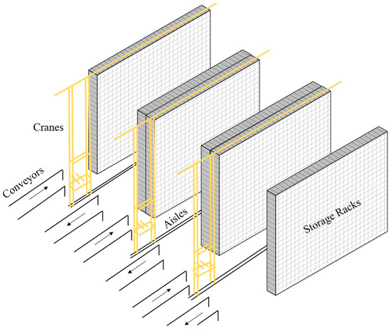
Figure 1.
Schematic diagram of the AS/RS in this study.
Therefore, on the one hand, incoming items can be assigned arbitrarily to any empty location in any aisle. On the other hand, there is a set of optional retrieval locations associated with the required items in each aisle. Moreover, in today’s just-in-time logistics and distribution environment, another big challenge is ensuring that the items are delivered on time. Typically, only the retrieval requests have due dates, so the items should be taken from the racks no later than the specified due date. Violation of the due date may delay subsequent loading and distribution processes, resulting in unacceptable satisfaction and high logistics costs (Scholz, Schubert, and Wäscher 2017) [4]. According to the classification of Boysen and Stephan (2016) [5], this problem corresponds to the tuple , where para denotes that we consider parallel cranes in the AS/RS. Thus, three decisions are required to solve the parallel crane scheduling (PCS) problem in this AS/RS to minimize the total tardiness of the requests: (1) how the retrieval requests are assigned and (2) sequenced to the cranes (request assignment and sequencing), and (3) which pair of storage and retrieval locations should be selected from multiple possible locations (storage/retrieval location selection). The PCS problem is NP-hard, since the problem of request sequencing and finding the best storage and retrieval location among those available is NP-hard (Meneghetti, Dal Borgo, and Monti 2015) [6]. In this research, we need not only to select the best storage/retrieval locations from multiple feasible locations, but also to consider which crane the requests should be assigned to and the sequence of the requests for each crane. We adopted the explicit-based approach by considering the three decisions of request assignment, sequencing, and storage/retrieval location selection simultaneously to enhance the algorithm’s efficiency. These three decisions are interrelated and interact, making it a challenging problem to optimize them simultaneously to minimize the total tardiness of the requests.
This problem is important because the efficiency of the entire supply chain is affected by the performance of warehouse operations, especially the storage and retrieval of items (Ballestín, Pérez, and Quintanilla 2020) [7]. Moreover, with the development of warehouse automation, an increasing number of enterprises are using this type of AS/RS to improve warehouse space utilization and operational efficiency. The decisions regarding request assignment, sequencing, and storage/retrieval location selection are logically interconnected. Only by considering these jointly can we achieve the overall optimization of system operation and minimize the tardiness of customer requests. Joint consideration has the potential to enhance customer satisfaction, reduce logistics costs, and improve the market competitiveness of enterprises. Previous research has often assumed that a multi-aisle AS/RS can be treated as several independent single-aisle AR/RSs, primarily investigating the SCS problem. This perspective involves sequencing requests on a single crane and potentially determining suitable storage locations (Gagliardi, Renaud, and Ruiz 2013; Nia, Haleh, and Saghaei 2017) [8,9]. However, managing a multi-aisle system globally, instead of independently handling multiple aisles, can significantly reduce the makespan of a set of requests (Gagliardi, Renaud, and Ruiz 2015) [10]. In this paper, we are motivated by real-world scenarios encountered at a major Chinese garment maker’s intelligent warehouse. Taking into account the current environment of parallel cranes and recognizing the advantages of globally managing a multi-aisle system, we adopt a global approach to managing multiple aisles and consider a set of available storage/retrieval locations in a unit-load AS/RS.
Our main contributions are as follows: First, we introduce a new complex and practical problem in multi-aisle AS/RSs, called the parallel crane scheduling (PCS) problem. This is the first time that the decisions of request assignment/sequencing and storage/retrieval location selection have been considered simultaneously. Furthermore, we introduce a new dynamic programming (DP) model combined with a mixed-integer linear programming (MIP) model to provide insight into the PCS problem. Second, considering the feature of location-dependent processing time, we transform this problem into a variant of the unrelated parallel machine (UPM) scheduling problem that minimizes the total tardiness of the requests. Meanwhile, a modified apparent tardiness cost (ATC) heuristic and an ant colony system (ACS) algorithm that employs two problem-specific local optimization operators are developed to solve this problem. Third, we generate new test instances and conduct extensive computational experiments for the problem. The experimental results verify that our algorithms provide excellent performance in PCS problem, and we also evaluate the performance of our ACS algorithm in solving the SCS problem. In addition, we can draw inspiration from the experiments that when designing operation schemes for multi-aisle AS/RSs, especially in large-scale multi-aisle AS/RSs, the global scheduling of multiple aisles should be considered to reduce the total tardiness.
The rest of this paper is organized as follows: In Section 2, we review the literature regarding the SCS problem in AS/RSs and the problem of unrelated machine scheduling. In Section 3, we define the PCS problem and give a numerical example to illustrate the problem. Then, a new mathematical model is introduced, and finally, we analyze how to transform the PCS problem into a variant of the UPM problem. In Section 4, a modified ATC heuristic and an ACS algorithm with local optimization are developed to solve the problem. In Section 5, computational experiments are conducted, and the experimental results are analyzed and discussed. Finally, in Section 6, conclusions and future study topics are introduced.
2. Literature Review
In past years, many scholars have reviewed the AS/RS literature from different perspectives (van den Berg and Gademann 1999; Roodbergen and Vis 2009; Gagliardi, Renaud, and Ruiz 2012; Boysen and Stephan 2016; Azadeh, De Koster, and Roy 2019) [5,11,12,13,14]. In a single-aisle AS/RS, the total throughput can be maximized by minimizing the crane’s travel time, which depends on two operational decisions: (1) the assignment of incoming items to storage locations, and (2) the sequencing decisions (Gagliardi, Renaud, and Ruiz 2013) [9]. Some of the literature studies a single decision in isolation (Lee and Kim 1995; Lee and Schaefer 1997; Emde, Polten, and Gendreau 2020) [15,16,17], but now more of the literature tends to optimize these two decisions simultaneously (Chen, Langevin, and Riopel 2008; Hachemi, Sari, and Ghouali 2012; Gagliardi, Renaud, and Ruiz 2013; Nia, Haleh, and Saghaei 2017) [8,9,18,19].
Thus, Section 2.1 reviews related work on unit-load AS/RSs from two perspectives: the request sequencing problem without considering location assignment, and the sequencing problem integrating location assignment.
2.1. The SCS Problem in AS/RSs
Sequencing problem without considering location assignment: The request sequencing problem without considering location assignment is to determine how to pair the storage and retrieval operations on the premise that the storage and retrieval locations are known. Lee and Kim (1995) [15] investigated the problem of scheduling storage and retrieval orders without considering location assignment under DC operations in a unit-load AS/RS. The objective was to minimize the weighted sum of earliness and tardiness penalties with respect to a common due date. Lee and Schaefer (1997) [16] studied the sequencing problem with dedicated storage, in which the storage requests are assigned to predetermined storage locations. Van den Berg and Gademann (1999) [11] addressed the request sequencing problem in a single-aisle AS/RS with dedicated storage. The static block sequencing method was used to minimize the travel time. Emde, Polten, and Gendreau (2020) [17] studied the SCS problem in the just-in-time production environment and transformed the request pairing and batch sequencing problem into a single batching machine scheduling problem, with the objective of minimizing the maximum lateness. We were particularly inspired by this study to regard our problem as a UPM problem.
Sequencing problem integrating location assignment: In a unit-load AS/RS, there are usually multiple opening locations, and the storage requests have no fixed target position. Given the list of retrieval requests and a set of items to store, the sequencing problem integrating location assignment is to pair the empty locations (one for each storage item) with the retrieval requests to minimize the total travel time. Han et al. (1987) [20] investigated this problem and proposed two methods for sequencing storage and retrieval requests in a dynamic situation. In the work of van den Berg and Gademann (2010) [21], these two methods were referred to as “wave sequencing” and “dynamic sequencing”, respectively. Lee and Schaefer (2007) [22] presented an algorithm that combines the Hungarian method and the ranking algorithm for the assignment problem with tour-checking and tour-breaking algorithms. Gagliardi, Renaud, and Ruiz (2013) [9] investigated the retrieval request sequencing and storage location assignment problem simultaneously in a unit-load AS/RS. They reviewed and adapted the most popular sequencing policies to dynamic contexts, and then proposed a “sequencing mathematical model” to solve the problem. Chen, Langevin, and Riopel (2008) [18] suggested that storage location assignment and the interleaving problem (LAIP) are logically interrelated. They addressed both problems in an AS/RS with a duration-of-stay-based shared storage policy. Hachemi, Sari, and Ghouali (2012) [19] dealt with the sequencing problem where the retrieval and storage locations are all not known in advance. An optimization method working step by step was developed. In the work of Nia, Haleh, and Saghaei (2017) [8], the authors dealt with a DC cycle “dynamic sequencing” problem in a unit-load, multiple-rack AS/RS. The objective was to minimize the total cost of greenhouse gas efficiency in the AS/RS.
All of the above literature focuses on a single-aisle AS/RS; only Gagliardi, Renaud, and Ruiz (2015) [9] investigated the request sequencing problem from the global perspective of multiple aisles. They proposed two multi-aisle sequencing approaches, finding that globally sequencing an m-aisle system instead of independently sequencing m single-aisle systems leads to important reductions in makespan. We review and summarize the above literature in Table 1. Since the paper of van den Berg and Gademann (2010) [21] simulated the effects of various storage assignment and request sequencing strategies, it is not listed separately in the table. Other studies involve different types of AS/RS, such as multi-shuttle AS/RSs, aisle-mobile crane AS/RSs, mini-load AS/RSs, and shuttle-based storage and retrieval systems (Sarker et al., 2007; Tanaka and Araki 2006; Popović, Vidović, and Bjelić 2012; Yang et al., 2013; Yang et al., 2015; Wauters et al., 2016; Singbal and Adil 2021; Marolt, Šinko, and Lerher 2022; Ekren and Arslan 2022; Küçükyaşar, Y. Ekren, and Lerher 2020) [23,24,25,26,27,28,29,30].

Table 1.
Summary of the related works.
In summary, we can conclude that that the literature investigating the problem of PCS to minimize the total tardiness of the requests is almost nonexistent. Most previous works studied the request sequencing problem of AS/RSs based only on a single aisle. However, in reality, most AS/RSs have multiple aisles, and only Gagliardi, Renaud, and Ruiz (2015) [9] investigated the problem of request assignment in this context. Considering the literature on minimizing total tardiness in an AS/RS, Emde, Polten, and Gendreau (2020) [17] suggested that the AS/RS literature focuses almost exclusively on the makespan objective; time windows that are common in real-world just-in-time environments are rarely considered in the literature. A few exceptions include Linn and Xie (2007), Lee and Kim (1995), and Emde, Polten, and Gendreau (2020) [15,17,31].
2.2. Unrelated Machine Scheduling Problem
In this research, we consider the multi-aisle AS/RS, whose scheduling problem includes not only sequencing requests but also assigning them to multiple cranes, which is similar to the parallel machine scheduling problem (Biskup, Herrmann, and Gupta (2008) [32]). Moreover, the processing time of the requests is different on each machine, allowing us to transform the PCS problem into a variant of the UPM problem (see Section 3.4 for details).
Thus, in this section, we review the related work of minimizing total (weighted) tardiness in the UPM problem. Unrelated machines can process jobs at different rates so that the jobs have different processing times on different machines (Yepes-Borrero et al., 2020 [33]). The decision of the UPM problem is to determine how the jobs are assigned and sequenced to the machines. Liaw et al. (2003) [34] used a branch-and-bound algorithm to solve the UPM problem of minimizing the total weighted tardiness, in which the ATC heuristic was used for the upper bound. Lin, Pfund, and Fowler (2011) [35] designed a genetic algorithm to minimize regular performance measures, including makespan, total weighted completion time, and total weighted tardiness. Lin, Lin, and Hsieh (2013) [36] proposed an ACS algorithm to solve the problem of scheduling the UPM to minimize the total weighted tardiness. Lin, Fowler, and Pfund (2013) [37] also developed heuristic and genetic algorithms to find non-dominated solutions to multi-objective unrelated parallel machine scheduling problems. Lin and Ying (2014) [38] proposed a multipoint simulated annealing heuristic algorithm to solve the UPM problem by simultaneously minimizing the makespan, total weighted completion time, and total weighted tardiness. Salazar-Hornig et al. (2021) [39] proposed a hybrid heuristic combining variable neighborhood search (VNS) with ant colony optimization (ACO) to solve the scheduling problem of nonrelated parallel machines with sequence-dependent setup times in order to minimize the makespan. Ulaga et al. (2022) [40] designed an iterative local search (ILS) method for solving the problem of scheduling parallel unrelated machines, which combined various improved local search operators and proved to be a simple but efficient method. Moreover, Ɖurasević et al. (2023) [41] provided a systematic and extensive literature review on the application of heuristic and metaheuristic methods for solving the UPMSP and outlined recent research trends and possible future directions.
3. Problem Description, Modeling, and Analysis
Here, we first describe the problem in Section 3.1 and give an example to illustrate the problem in Section 3.2. Then, we present two related models of the problem in Section 3.3. In Section 3.4, we show how to transform the PCS problem into a variant of the UPM problem and analyze the difference between the two problems.
3.1. Problem Description
Let be the set of storage requests and be the set of retrieval requests. The number of retrieval requests is equal to the number of storage requests (Hachemi, Sari, and Ghouali 2012) [19], and each retrieval request has a due date . Let be the index of retrieval requests in set . Let be the set of cranes; it can also be said that there are aisles in total. We assume that the crane executes the task in DC mode, so the DC time refers to the travel time of executing the dual command cycle of storage and retrieval requests (Nia, Haleh, and Saghaei 2017) [8]. The PCS problem can be stated as follows: Schedule a set of n requests on a set of cranes, and select the storage and retrieval locations for these requests. Therefore, a solution for this problem consists of three parts: First, denotes the optimal solution of retrieval requests’ sequence on each machine. Second, denotes the optimal solution of corresponding selected storage locations. Third, denotes the optimal solution of corresponding selected retrieval locations, so the complete solution of the problem is . Thus, the tardiness of the retrieval request can be calculated by max, where denotes the completion time of retrieval request . Finally, the objective is to minimize the total tardiness of the requests: . The following assumptions are used throughout this paper:
- All of the storage requests are processed in an FCFS manner, and all of the retrieval requests can be resequenced. The crane can carry only one unit load and executes requests in DC mode, which starts from the IO station and returns to the IO station after completing one storage task and then one retrieval task.
- Since we consider the shared storage strategy, items can be stored in any empty location on any rack, and items to be retrieved can be located in multiple aisles and on multiple positions of a rack. Therefore the locations-to-product ratio is .
- To be able to execute a DC, the number of storage and retrieval tasks must be equal. Without loss of generality, there are no items of the same type in the storage and retrieval list. If it exists, it can be directly taken out.
- The initial state of the rack locations and the due date of each request are known with certainty.
- The crane can move simultaneously both vertically and horizontally at constant speeds. The travel time of the crane to reach any location in the rack is calculated by the Chebyshev metric, and the pick-up and set-down times are ignored since they are inconsequential for optimality.
3.2. Numerical Example
For the sake of better understanding, we give a numerical example to illustrate the PCS problem. In this example, the unit-load AS/RS has cranes , indicating that there are two aisles in total, consisting of four racks: . Each rack is with 25 locations, for a total of 100 locations. The initial state of each rack is shown in Figure 2. We assume that the height and width of each location are both 1 m, and that the horizontal and vertical traveling speeds of the crane are both 1 m/s. Six retrieval requests and six storage requests = are received. The due dates of the retrieval requests are 7, 9, 11, 8, 10, and 14, respectively, and the storage requests are processed in an FCFS manner.
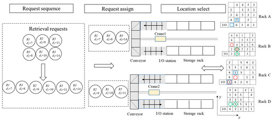
Figure 2.
An example of the PCS problem. Three decisions need to be made: request sequencing, request assignment to cranes, and selection of storage and retrieval locations. Values of d indicate the due date of each request. The number inside the rack is the type of item; empty locations have no number. The solution of location selection is displayed on the rack. Note that the two locations marked with the same shape in a rack are processed in the same DC, and the color of the label indicates the order in which the DC is executed: the first DC is highlighted in red, the second is blue, and the last is green.
The three decisions that we made for this example are shown in Figure 2. A feasible and optimal solution for this example is as follows: = [R1, R3, R3; R2, R1, R5]. = [(B, 1, 3), (A, 1, 1), (B, 2, 2); (C, 2, 2), (C, 1, 1), (D, 1, 2)]. = [(B, 2, 2), (A, 2, 2), (B, 2, 1); (C, 1, 1), (C, 2, 3), (D, 2, 2)].
Table 2 shows the corresponding solution of the example. First, crane 1 stores an item of type 4 to the initially empty location (B, 1, 3) and retrieves an item of type 1 from location (B, 2, 2). Second, crane 1 stores an item of type 6 in empty location (A, 1, 1) and retrieves an item of type 3 from location (A, 2, 2). Third, crane 1 stores an item of type 4 in the vacated empty location (B, 2, 2) and retrieves an item of type 3 from location (B, 2, 1). The processing times of the three DCs are 6, 4, and 5, respectively, and the corresponding due dates for each DC are 7, 8, and 14. Therefore, the tardiness on crane 1 is 3. The other three storage requests and retrieval requests are handled by crane 2, whose processing times for each DC are 4, 6, and 5, respectively. The corresponding due dates are 9, 10, and 11, so the tardiness for crane 2 is 4. Finally, we can calculate the total tardiness .
Table 2.
Solution of the numerical example.
3.3. Mathematical Models
Since the empty location generated by the retrieval operation is instantly available, the rack state, used as an input parameter, changes with each location selection decision, which makes it difficult to build a complete model by using an MIP model alone. Therefore, referring to the works of Yang et al. (2013) and Hachemi, Sari, and Ghouali (2012) [19,26], we introduce a DP model combined with an MIP model to describe the PCS problem.
The DP model is used to describe request assignment and sequencing decisions and to depict the dynamic change in the location state. According to the total number of requests n, the DP model is divided into n stages. In stage b, the DP model needs to arrange b + 1 requests, so that there are permutations. In each permutation, an MIP model is established to select the storage and retrieval locations under the current state of rack locations, and then to calculate the processing time and tardiness of the request. When the request is scheduled, the model should update the rack location state, and the updated rack location state is used as the input state for the next stage.
3.3.1. Parameters
| Represents a collection of retrieval requests. | |
| Index of retrieval items, . | |
| Index of item type of retrieval requests by customers. means the item type of retrieval request in is . | |
| Indicates the due date for the th retrieval request. | |
| Tardiness of retrieval request . | |
| Rack in aisle, . | |
| Horizontal location index, . | |
| Vertical location index, . | |
| Horizontal travel velocity of crane. | |
| Vertical travel velocity of crane. | |
| Index of item type, . | |
| Crane in , where is the set of cranes, . | |
| Processing time of DC on crane in stage . | |
| A big positive integer. | |
| Set of empty locations on the shelf that crane is responsible for before stage when the scheduled request sequence is . represents the initial set of empty storage locations on the shelf that crane is responsible for when and . , . | |
| Set of locations on the shelf containing items of type that crane is responsible for before stage , when the scheduled request sequence is . represents the initial set of storage locations on the shelf containing items of type that crane is responsible for when and ., , . | |
| Completion time of DC on crane in stage . | |
| Decision variable equal to 1 if in stage , the storage location on the th row shelf responsible for crane and the storage location containing the th retrieval item form a DC. | |
| Travel time between storage location and retrieval location . |
When the decision variable is 1, it indicates that in stage , the storage location on the th row shelf responsible for crane and the storage location containing the th retrieval item form a DC; represents the travel time between storage location and retrieval location , and its value is calculated by the Chebyshev formula, as shown in Formula (1):
3.3.2. DP Model
- Stage: The stages in a DP model are divided according to the number of requests, i.e., requests represent stages.
- State variables: , , .
- Decision variables: .
- State transition equation:
- Optimal value function:represents the minimum total tardiness when request ranks one behind the set containing requests. .is the boundary condition representing the total tardiness obtained by scheduling each request when the set .
The optimal value function is expressed as follows:
In each stage of the dynamic programming model, the IP model is solved to select the storage and retrieval locations for the retrieval request with the current state of rack locations and then calculate the tardiness of the request. denotes the tardiness of request , which can be calculated using the following IP model. In the IP model, the input states are .
3.3.3. Integer Programming Model
Objective (7) is to minimize the tardiness of request . Constraint (8) ensures that only one empty and one retrieval location, both on the same rack of a crane, are selected to perform the DC cycle. Constraints (9) and (10) ensure that the storage items are stored in empty locations and the retrieval location contains the item of request . Constraint (11) determines that the processing times of the retrieval request on crane equal the travel time for the storage and retrieval locations (DC); it is calculated by the Chebyshev metric. Constraint (12) represents the processing time of retrieval request r on crane . Constraint (13) represents the completion time of the retrieval request on crane .
From the DP model, we can observe that there are permutations in stage ; therefore, the DP model needs to solve MIP models in stage , and a total of MIP models must be solved in all stages. It can be seen that the computational complexity of the DP algorithm is very high, and with an increasing number of requests, the computational complexity greatly increases. Therefore, we designed a constructive heuristic and ACS algorithm to solve the problem.
3.4. Reduction to UPM Problem
In the following section, we show how to transform the PCS problem into a variant of the UPM problem. We can interpret the z cranes as z parallel machines, and we regard a crane executing a DC as a machine processing a job. Thus, the travel time of the crane to execute the DC becomes the processing time. Due to the different states of each shelf, the processing time of each request on each crane is variable. Thus, we can transform the problem into a variant of the UPM problem that minimizes total tardiness. However, the location-dependent processing time makes our problem different from the UPM problem.
Location-dependent processing time: In the classic UPM problem, the processing time of the job is known and constant, but in our case, the processing time of the requests depends on the choice of storage and retrieval locations, which is calculated by the Chebyshev metric. Since we consider the dynamic update of the rack state, the processing time of the request changes dynamically with the update of the rack locations; that is, after one job is assigned to the aisle, the rack state is updated. We need to reselect a pair of storage/retrieval locations for the unscheduled requests under the new rack state and recalculate the processing time.
4. Solution Methodology
As mentioned above, the PCS problem is NP-hard, the computational complexity of using an exact algorithm to solve this problem is very high, and the problem’s decisions are interrelated and interact with one another, which implies that constructive algorithms are suitable for solving this problem (Zhang, Jia, and Li 2020; Shao, Shao, and Pi 2021) [42,43]. The ACO algorithm, as a constructive metaheuristic, performs well in solving combinatorial optimization problems, especially in machine scheduling problems (Xu, Chen, and Li 2012; Engin and Güçlü 2018; Li, Gajpal, and Bector 2018; Tavares Neto, Godinho Filho, and da Silva 2013) [44,45,46,47]. Thus, the current paper solves this problem efficiently by employing a constructive solution framework. Considering the feature of location-dependent processing time and the objective of minimizing the total tardiness time, a modified ATC (MATC) heuristic (Section 4.1) and an ACS algorithm with a problem-specific local optimization (Section 4.2) are proposed.
4.1. A Modified ATC-I Heuristic
In this study, we transformed the PCS problem into a variant of the UPM problem, with the objective of minimizing the total tardiness. Thus, we adapted the ATC-I heuristic to solve this problem, which is a state-of-art heuristic proposed by Lin, Pfund, and Fowler (2011) [35]. The modified ATC-I (MATC) heuristic is described below.
Because the problem features location-dependent processing time, firstly, we have to determine the processing time of each job on each crane; that is, we must select a pair of storage and retrieval locations and calculate the DC time. We propose an effective strategy for storage and retrieval location selection, called Algorithm 1. It first selects the retrieval location that is closest to the I/O point and then selects a feasible empty location that can minimize the DC time. Once a pair of locations is determined, the processing time can be calculated. Algorithm 1 is defined as follows:
| Algorithm 1 Local Search |
| Initialization: Let be the set of retrieval requests, be retrieval request in , and be the total number of retrieval requests. Let be crane in , and the total number of cranes be . for do for do
end for Output the processing time . |
Secondly, we need to sequence the requests and select a priority request. In MATC, we use the ATC rule to determine the order of the requests. The ATC rule is a well-known heuristic for minimizing total weighted tardiness in the single machine scheduling problem. Moreover, to verify the ATC performance, we compare the ATC with other important and effective sequencing rules in computational experiments (see Section 5.3 for details). Next, we need to assign the selected request to a crane. In this step, we manage multiple aisles globally instead of managing each independently. The MATC heuristic considers the rack state and the processing time of the request on each crane when assigning the request to a crane. We also verify the performance of globally managed multiple aisles in computational experiments (see Section 5.4 for details). Finally, we assign the priority request to the selected crane and update the states of the corresponding storage and retrieval locations. In the MATC heuristic, since the selection of the current request will change the rack states, it will then influence the processing time of subsequent unscheduled requests. Therefore, once the requests are assigned to cranes, the processing time of unscheduled requests needs to be recalculated. The detailed steps of the MATC heuristic are as follows:
Step 0: Let be the set of retrieval requests; let be the completion time of the request that has been scheduled on crane . Initially, set , .
Step 1: Select the storage and retrieval locations and calculate the processing time for each retrieval request on each crane m by Algorithm 1.
Step 2: Determine the first available crane , i.e., .
Step 3: Sequence the requests according to the ATC index and choose the retrieval request with the maximum ATC index (), where the ATC index . In the ATC index, is a scaling parameter, and is the average processing time of the requests on crane .
Step 4: Assign request to crane. (1) If assigning request to crane m would not lead to a delay (), for request find crane with minimal processing time (). (2) If the completion time is greater than the due date of the request (>), for request find crane with minimal tardiness ().
Step 5: Schedule request to crane , update , and set .
Step 6: Update the state of the rack, and recalculate the processing time for unscheduled retrieval request on crane using Algorithm 1.
Step 7: Repeat Steps 2–6 until all retrieval requests are scheduled.
4.2. Ant Colony System Algorithm for the PCS Problem
We modified the ACS algorithm proposed by Lin, Lin, and Hsieh (2013) [36] to our problem. In addition, a problem-specific local optimization was designed to improve the quality of the solution for location selection. The detailed steps of the ACS are as follows:
4.2.1. Solution Construction
Location Selection
Through Algorithm 1, as mentioned above, we can determine the processing time of the request on each crane.
Initial Crane Selection
Initial crane selection means determining the first available crane , i.e., .
Priority Retrieval Request Selection
After the crane has been selected, each ant must select the next retrieval request under the guidance of the heuristic information and pheromone trails, defined by Equation (15):
The definition of heuristic information is usually based on specific knowledge of the problem. The ATC rule is a well-known heuristic for minimizing the total weighted tardiness in the single machine scheduling problem, and it comprehensively considers the WSPT (weighted shortest processing time) and MS (minimum slack) rules (Pinedo 2016) [48]. Therefore, the ATC rule is utilized in heuristic information in combination with pheromone trails to determine the next request. Thus, for our problem, we define the heuristic information as the ATC index, . The pheromone trail represents the expectation of selecting a priority request on crane . Let be a random number from the uniform distribution , and let be a user-specified number such that . When , each ant selects a priority request that maximizes the value of . Otherwise, the ant randomly selects the priority request from the probability distribution formed by the probabilities , as given in Equation (16).
Crane Assignment
If assigning request to crane would not lead to a delay (<), for request find crane with minimal processing time (). If the completion time is greater than the due date of the request (>), for request find crane with minimal tardiness (). Next, schedule request in the first available sequencing position on crane and update the retrieval request set . Then, the ACS updates the state of the rack and recalculates the processing time of unscheduled retrieval request on crane using Algorithm 1. In the ACS algorithm, each ant must consider the processing time when selecting the request and assigning a request to a crane in each iteration, so it is necessary to recalculate the processing time of unscheduled requests after updating the rack location states. Therefore, the ACS algorithm is expected to require a high computational effort.
Update of Local Pheromone Trails
The update of pheromone trails includes pheromone trail deposition and pheromone trail evaporation. The pheromone deposit guides later ants to build better solutions, and pheromone evaporation can prevent all ants from quickly concentrating on a poor solution, which helps ants to explore new solution spaces and find better solutions.
In this paper, the algorithm uses both local pheromone updates and global pheromone updates. Updating the local pheromone makes the pheromone on the visited solution component decrease every time an ant selects the priority request on the initial crane, which reduces the probability of other ants selecting the component and increases exploration. The local pheromone trail is updated as follows:
After crane reselection, the pheromone on the visited solution component is updated by Equation (16). Here, ξ represents the local pheromone evaporation rate of the pheromone trails ; is the initial pheromone trails, defined as ; is the number of ants; and is the total tardiness obtained by the MATC heuristic.
The pseudocode for the solution construction procedure is summarized below:
Step 1: Initially, let the retrieval requests set , and let be the completion time of the request that has been scheduled on crane , . Initialize .
Step 2: Initial crane selection.
Step 3: Priority retrieval request selection. Select a retrieval request based on the following equation , where and is a probability distribution with .
Step 4: Crane assignment.
Step 5: Update of the rack state. Set . Reselect storage and retrieval locations and recalculate the processing time for unscheduled requests on crane using Algorithm 1.
Step 6: Update of local pheromone trails.
Step 7: Repeat Steps 2–6 until all requests are assigned.
4.2.2. Local Optimization
After the ant has constructed a solution, a local optimization method is used to improve the quality of the solution. In this section, we first propose two problem-specific swap operators for the local optimization. Due to the nature of the shared storage policy (i.e., the empty location generated by a retrieval operation is instantly available), the solution obtained by the ACS algorithm has the priority relationship constraint. Therefore, we introduced a priority relation of locations and defined the feasible regions of the two operators to generate the feasible solution.
Two Swap Operators
The solution obtained by the ACS algorithm is composed of the retrieval requests sequenced on each crane and the corresponding storage and retrieval locations. Therefore, new solutions can be obtained by swapping the order of the storage or retrieval location on the basis of the incumbent solution. Thus, we developed two swap operators. Figure 3 takes a solution as an example to show it.
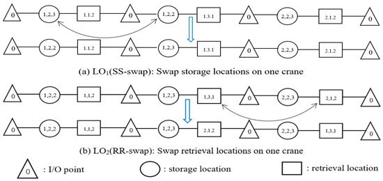
Figure 3.
Two swap operators.
- LO1 (SS-swap): Swap the storage location of two DCs on one crane. The sequence of retrieval requests does not change, but the processing time will change. This swapping can increase the exploration of solutions for storage location selection.
- LO2 (RR-swap): Swap the retrieval location of two DCs on one crane. The sequence and the processing times of the retrieval requests change. This swapping increases not only the exploration of solutions for location selection but also the exploration of solutions for request sequencing.
For each ant solution, the local optimization method selects one of the two operators , in an adaptive way (Hemmelmayr, Schmid, and Blum 2012) [49]. The counters are used to keep track of the performance of the two operators. All counters are set to 1 initially. When the local optimization solution is better than the incumbent solution, then the swap operator that was used in the corresponding local optimization step is incremented. We set probabilities , and an operator is determined through the roulette wheel rule. After the operator is determined, the local optimization method selects the best solution in the neighborhood.
Priority Relationship Constraint
Using the ACS algorithm, we can obtain the set of the storage location solution and the set of the retrieval location solution . Let be the storage location in set . Let be the retrieval location in set Since we apply a shared storage policy that can reuse the empty location generated by the retrieval operation, the order of locations in the solution obtained by the ACS algorithm has a priority relationship. We define the following priority relationship:
Definition 1.
Fixed priority relationship: If one empty location yielded after performing a retrieval operation is used for the later storage operation, the relationship between two operations is called a fixed priority relationship, which means the priority relationship cannot be changed. If the priority relationship did change, it would lead to an infeasible solution. This priority relationship is represented by a tuple , which means the retrieval operation must have fixed precedence over the storage operation.
To clarify these priority relationships, we introduce a priority relationship graph G = (V, C, I).
- V is the set of nodes corresponding to DCs on one crane in a solution.
- C is the set of directed connection arcs. There is a directional connection arc between each pair of consecutive nodes, indicating the order of storage and retrieval locations in the solution, as indicated by a solid arrow.
- I is the set of directed fixed priority connection arcs; these priority relationships cannot be changed. The retrieval operation at the end of the priority arc must be executed prior to the storage operation at the beginning of the arc, which is represented by a dotted arrow.
Example 1.
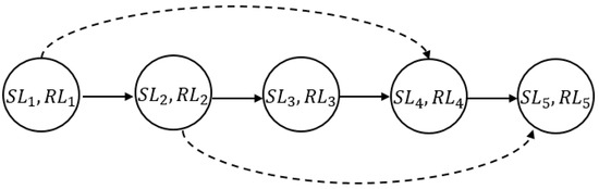
Assume that the storage and retrieval location solution of crane 1 obtained by the ACS is , . The first retrieval location is , which is used as the fourth storage location , and the second retrieval location is , which is used as the fifth storage location . Thus, the fixed priority relationship is . Figure 4 illustrates the fixed priority relationships of the example.
Figure 4.
Diagram of the fixed priority relationships in Example 1.
The Feasible Region of the Two Local Optimization Operators
In the local optimization, fixed priority relationships must be considered to ensure that feasible solutions are produced. If local optimization is performed without considering the fixed priority relationship, an infeasible solution will be generated, which will take a long time to repair. Therefore, to improve the algorithm’s efficiency, we executed a local optimization method only within the feasible regions of the operators. Next, we propose two propositions to describe the feasible regions of the two operators.
Proposition 1:
When executing the LO1 (SS-swap) operator on crane m, assume that the retrieval location has a fixed priority over the storage location in the solution; that is, , and . Then, the feasible region of LO1 (SS-swap) operator is as follows:
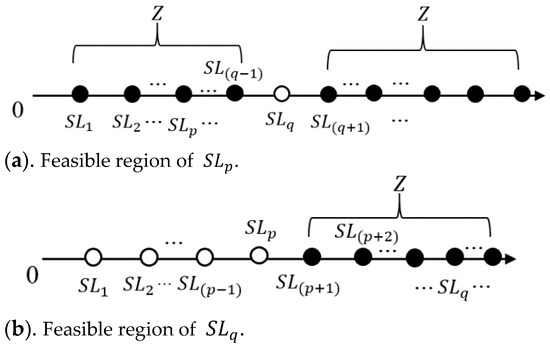
Figure 5.
Feasible regions of LO1 (SS-swap).
Proof:
In the first case, if the storage location is swapped with the storage location, the storage location and retrieval location are in one DC. When performing this DC, the storage location on the rack is occupied by an item. In the second case, if the storage location is swapped with the other storage location before the request, the storage location is executed first in order, but at this time the storage location on the rack is in the state of being occupied by items. □
Proposition 2:
When executing the LO2 (RR-swap) operator, assume that the retrieval location has a fixed priority with the storage location in the solution; that is, , and . Then, the feasible region of the LO2 (RR-swap) operator is as follows:
The feasible region of is shown in Figure 6a. For , the feasible region of this operator is shown in Figure 6b. The proof is similar to that of Proposition 1.
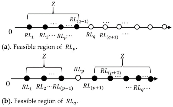
Figure 6.
Feasible regions of LO2 (RR-swap).
4.2.3. Update of Global Pheromone Trails
In the ACS algorithm, only the global best solution is used to update the pheromone trails after each iteration. The update of is defined as follows:
where represents the global pheromone evaporation rate of the pheromone trails (), and , where is the best solution value found so far.
The pseudocode for our Algorithm 2 is summarized below:
| Algorithm 2 ACS Algorithm | |
| 1: | Initialize: Retrieval request , , for ; denotes the total tardiness of the solution in . The maximum number of iterations is , the global evaporation rate is , the local evaporation rate is , the relative importance of the pheromone trails is , and that of the heuristic information is |
| 2: | Select storage and retrieval locations and calculate the processing time for each request on each crane using Algorithm 1. |
| 3: | , , . |
| 4: | for do |
| 5: | for each ant do |
| 6: | Call the solution construction procedure to construct the solution. |
| 7: | Use the roulette wheel rule to choose one operator , to execute the local optimization. |
| 8: | if then |
| 9: | . |
| 10: | end if |
| 11: | end for |
| 12: | Update the global pheromone by Equation (18). |
| 13: | Update the global best solution. |
| 14: | |
| 15: | end for |
| 16: | Output the global best solution. |
5. Computational Experiments
In this section, several computational experiments were conducted to assess the performance of our proposed algorithms through algorithm comparisons. First, we generated our benchmark according to related studies (Section 5.1). Second, a series of pilot experiments determined the important parameter values that performed well in most ACS instances (Section 5.2). Then, we evaluated the performance of the sequencing strategy (Section 5.3), aiming to validate that considering the request assignment globally in a multi-aisle AS/RS provides benefits in terms of the total tardiness of the requests (Section 5.4). We examine the capability of the proposed Algorithm 2 in handling both small and large instances in Section 5.5. In the last experiment, we explored the performance of the request sequencing and location selection strategy of the ACS in addressing the SCS problem (Section 5.6). Our algorithms were coded using MATLAB R2020a software. All tests were conducted on a desktop PC with a 2.4 gigahertz Pentium processor and 4 gigabytes of RAM.
5.1. Instance Generation
Unfortunately, real-life example data are not available, and there are no benchmark instances in the literature that consider the PCS problem, so we refer to similar AS/RS papers to generate our own test instances. The details of our instance generator are described below:
- Layout: For small instances, the AS/RS contains two aisles with four racks. The number of rack locations (layer × tier) is set to 5 × 6 (30), 5 × 8 (40), and 5 × 10 (50) (Yang et al., 2015; Hachemi, Sari, and Ghouali 2012) [19,27]. For large instances, the AS/RS contains four aisles with eight racks. The number of rack locations (layer × tier) is set to 10 × 10 (100), 10 × 20 (200), and 12 × 25 (300) (Yang et al., 2015; Nia, Haleh, and Saghaei 2017) [8,27]. The crane moves horizontally and vertically at 1 m/s. The initial state of each rack is randomly generated, with the utilization rate of each rack being 80%, which means that 20% of the rack locations are vacant. There are 20 types of items in the warehouse.
- Request: The number of small and large instance requests is set to 60 and 300, respectively. The due dates are usually generated based on the processing time of the requests. In this study, due dates were generated from a uniform distribution , where represents the average processing time of requests on cranes, expressed as , where is the processing time of request on crane (Lin, Pfund, and Fowler 2011). In this section, we apply Algorithm 1 to determine the processing times of requests and then calculate the average processing time . As can be seen, the tightness of the due dates depends on and . is the average tardiness factor, and is the relative range of the due dates. and are set to 0.4 and 0.8, respectively (Lin, Pfund, and Fowler 2011) [35], so there are four combinations for due dates: [T, R] = [0.4, 0.8], [0.4, 0.4], [0.8, 0.8], and [0.8, 0.4]. Table 3 summarizes the problem parameters and their corresponding values. For each parameter combination, 10 problem instances were generated and the results were obtained from 10 runs for each test instance.
Table 3. Parameter settings for generated PCS problem instances.
5.2. Parameter Settings
There are multiple parameters that will influence the search performance and the convergence quality in the ACO algorithm. In the ACS, since a pseudorandom transfer strategy is introduced and , the parameters that have the most important influence on the algorithm’s performance are , , and . Therefore, in this section, we conducted experiments to determine the main parameters in the ACS. The values of the other parameters were as follows: number of ants , maximum number of iterations , and the value of the ATC index in heuristic information was set to 0.6. We used the approach mentioned by Miao et al. (2021) [50] to determine the values of the parameters. We set the ranges of these parameters to , , and , and the default values of the groups of parameters were set to , , and , respectively. Only one parameter could be changed in each group experiment, and the other parameters were the defaults. We ran each group of parameters ten times and then compared the averages. The experimental results shown in Table 4 reveal that when , , and , the ACS can obtain the best solutions.
Table 4.
Experimental results for Algorithm 2 parameters.
5.3. Evaluation of the Performance of the Sequencing Rule
In this part of the study, we verified that sequencing requests can lead to significant improvements with respect to the total tardiness, and that ATC-based sequencing rules can obtain better solutions than other sequencing rules. We compared the ATC rule with other existing sequencing rules (MDD (modified due date), EDD (earliest due date), and FCFS), without considering the global assignment of requests. The EDD is a simple rule that sequences the requests in increasing order of their due dates. The MDD rule sequences the requests based on the earliest modified due date. FCFS sequences the requests in the order in which they arrive. The reason we that chose these sequencing rules is that they are important and effective rules for minimizing tardiness in machine scheduling problems, and they can be modified to apply to our problem.
We first sequenced the requests according to the abovementioned rules, and then we evenly assigned the sorted requests to cranes according to the sequence. The computing time of any of the above sequencing rules takes less than one second, and that time can be neglected. We compared the average relative percentage deviations (RPDs) from our ACS according to the following expression: , where is the total tardiness obtained by the above sequencing rules without considering the global assignment of requests, while is the total tardiness obtained by our Algorithm 2. Table 5 shows the results in small and large instances. We can see that ATC deviated 74.24% from the ACS, MDD deviated 84.73% from the ACS, EDD deviated 135.45% from the ACS, and FCFS deviated 196.12% from the ACS for small instances. Meanwhile, ATC deviated 178% from the ACS, MDD deviated 182.09% from the ACS, EDD deviated 200.20% from the ACS, and FCFS deviated 227.41% from the ACS for large instances.
Table 5.
Evaluation of the sequencing strategy for small and large instances.
We can conclude from the table that the ATC-based sequencing rule outperforms other rules, and MDD outperformed EDD, while EDD outperformed FCFS. Both ATC and MDD consider the processing time of requests when sequencing requests. In our testing, it can be seen that ATC was slightly better than MDD. Since EDD only considers the due dates without taking the processing time into account, solutions obtained by EDD-based algorithms are of very poor quality. The FCFS-based approach yielded the worst-quality solutions.
5.4. Evaluation of the Performance of Globally Managing Multi-Aisle AS/RSs
In this study, we globally managed a multi-aisle AS/RS instead of managing the multiple aisles independently. Thus, in this part of the study, we verify that in an AS/RS with shared storage, managing multiple aisles globally rather than independently can significantly reduce the overall tardiness of the requests.
By comparing the above request sequencing strategies, we can conclude that the ATC-based rule is the best. Therefore, in this section, we first sort the requests according to the ATC and then compare the quality of the solutions obtained by the global assignment policy and the independent assignment policy.
- Global assignment policy: Managing multi-aisle AS/RSs globally means considering the state of each rack when assigning requests to cranes and taking the processing time of the requests on each crane into consideration. Sorting requests based on the ATC rule and then assigning requests globally to cranes using the MATC heuristic.
- Independent assignment policy: Managing multi-aisle AS/RSs independently means evenly allocating requests to cranes in the sorted order regardless of the rack states and the processing time of requests for each crane.
Table 6 shows the RPD of the assignment policy in small and large instances. From the table, we can observe that for small instances, the independent assignment policy deviated 74.24% from the ACS, while the global assignment policy deviated 8.23%. For large instances, the independent assignment policy deviated 178% from the ACS, while the global assignment policy deviated 5.83%. We can conclude that assigning requests globally can significantly improve the solution compared to assigning requests independently.
Table 6.
Evaluation of the assignment strategy for small and large instances.
From these two experiments, we receive the insight that when designing operation schemes for multi-aisle AS/RSs, especially large-scale multi-aisle AS/RSs, global scheduling of multiple aisles should be used to reduce the total tardiness of the requests.
5.5. Evaluation of the Performance of the Algorithm 2
In this section, we evaluate the quality of the solutions obtained by the ACS in small and large instances. As mentioned above, the literature dealing with the PCS problem is almost nonexistent. Therefore, to evaluate the performance of the Algorithm 2, we must modify the state-of-the-art algorithm to use as a reference for our algorithm. We compared our Algorithm 2 with the step-by-step program (SSP) proposed by Hachemi, Sari, and Ghouali (2012) [19] and the genetic algorithm (GA) proposed by Lin, Pfund, and Fowler (2011) [35].
The SSP is a nested algorithm designed to solve the problem of request sequencing and storage/retrieval location selection in a single-aisle AS/RS. Its objective is to minimize the total travel time of the crane. It can be seen that this problem is very similar to our problem, with the difference being that this problem does not consider the request allocation. We modified the SSP model, changing the objective of the model and then using Gurobi to solve the model for our problem. Since we transformed the problem into a UPM problem, we wanted to know how well other algorithms that solve UPM problems would perform when solving our problem. Thus, we modified the GA proposed by Lin, Pfund, and Fowler (2011) [35], who solved a UPM scheduling problem that minimizes total tardiness. In our GA, the initial solution, crossover, and mutation operators are consistent with those in the literature. The difference is that after the request allocation and sequencing solutions are generated, we use Algorithm 1 to select the storage and retrieval locations on the corresponding crane. The GA parameters used in this study duplicate those in the literature.
In summary, we modified two previous algorithms to solve our problem. Because Gurobi is very time-consuming on large instances, we only compared the results with the GA algorithm in large instances, while in small instances we compared them against both the SSP and GA. The RPD is computed according to the following expression: . Here, is the total tardiness obtained by the SSP or GA, and is the total tardiness obtained by the ACS.
5.5.1. Comparison of Algorithms in Small Instances
For small instances, we compared our ACS with both the SSP and GA. Table 7 gives the computational results and CPU times. The “time” columns show the average CPU times in seconds, and “ACS_0” denotes the ACS without local optimization. We can observe that ACS_0 deviated 4% from the ACS, which suggests that local optimization plays a role in improving the solution quality. The SSP deviated 57% and the GA deviated 6.1% from our proposed Algorithm 2, respectively. Our ACS is slightly better than the GA, while for problem classes with a small number of rack locations (5 × 6) and loose due dates (T = 0.4, R = 0.8), the GA is better than the ACS (RPD = −0.014). We can conclude that the ACS outperforms ACS_0, the SSP method, and the GA in terms of total tardiness.
Table 7.
Comparison of the ACS with the GA and SSP for small instances.
5.5.2. Comparison of Algorithms in Large Instances
The computational results and the average CPU times for large instances are presented in Table 8. As shown in the table, the ACS without local optimization deviated 2.3% from the ACS, the GA deviated 37.1%, and the ACS is much better than the GA. The quality of the solution obtained by the GA is very poor in large-instance problems, and we can observe that, whether in terms of tight or loose due dates, the ACS outperformed ACS_0 and the GA.
Table 8.
Comparison of the ACS with the GA for large instances.
In addition to the quality of the solution obtained by the algorithm, the computation time should also be considered when evaluating the algorithm. Table 7 and Table 8 show that the ACS computing times depend on the numbers of requests and total locations. When the total location count increases, the number of locations containing retrieved items and the number of empty locations also increase, so when determining a pair of storage and retrieval locations, more possible DCs must be checked. For problem classes with small instances, the average computing time using the ACS is 89.167 s, while that of the GA is 258.267 s and that of the SSP is 21,348 s. For problem classes with large instances, the ACS’s average computing time is 1834.333 s, while the GA’s is 1991 s. We can conclude that our Algorithm 2 is superior to the GA and SSP not only in the quality of the solution, but also in terms of computing time.
5.6. Performance of ACS on Single Crane Scheduling Problem
In order to further evaluate the performance of the request sequencing and location selection strategy in the ACS, we modified it to solve the SCS problem that sequences the requests and selects the storage/retrieval locations. The modified ACS was compared with the SSP algorithm, but since our problem’s objective is inconsistent with the SSP’s, we had to modify the SSP. We used parameters consistent with those in the work of Hachemi, Sari, and Ghouali (2012) [19], so in this part of the experiment we set the rack size to 5 × 10 (50) and the number of requests to 60. We processed each instance ten times to obtain the averages shown in Table 9. From the table, we can see that the ACS performs better than the SSP. This experiment confirms that the performance of the request sequencing and location selection strategy in the ACS is also good in solving the single crane scheduling problem.
Table 9.
Comparison of the ACS and SPP on the single crane scheduling problem.
6. Conclusions and Future Work
This paper introduced and investigated the parallel crane scheduling (PCS) problem in a multi-aisle AS/RS with shared storage. The objective was to minimize the total tardiness of the retrieval requests. We proposed a new dynamic programming model combined with an integer programming model to illustrate the problem. Considering the features of the problem, we transformed the problem into a variant of the unrelated parallel machine scheduling problem. To solve the problem efficiently, a heuristic based on ATC sequencing rules and an ACS algorithm with local optimization were proposed.
Through numerical experiments, we found that the global scheduling of aisles can lead to significant improvements in total tardiness compared to considering aisles independently. Therefore, globally scheduling aisles should be considered when designing an operation scheme for multi-aisle AS/RSs. We verified that the ACS algorithm performs better than the GA and SSP algorithms. We also demonstrated that the ACS sequencing and location selection strategy is feasible and performs well in solving the single crane scheduling problem.
The major limitation is that the algorithm is currently applicable to scenarios designed for parallel crane configurations, and it cannot be directly applied to scenarios involving heterogeneous parallel cranes or multi-shuttle AS/RSs, among other variations. Furthermore, because the ACO algorithm belongs to the constructive-based metaheuristic framework, its solution time is relatively longer. Nevertheless, it can still attain satisfactory solutions within an acceptable and reasonable timeframe. Future research could focus on designing more efficient algorithms to solve the PCS problem, such as simulation annealing (SA) algorithms, greedy randomized adaptive search procedures (GRASPs), and particle swarm optimization (PSO). Moreover, future research could explore the request assignment and sequencing and the storage and retrieval location selection problem in other AS/RS types, such as the multi-shuttle AS/RS, which is also an interesting, realistic, and challenging problem.
Author Contributions
Conceptualization, R.X. and Y.T.; methodology, R.X. and H.C.; software, R.X. and H.C.; validation, R.X. and H.C.; formal analysis, R.X. and Y.T.; investigation, R.X. and H.C.; resources, R.X.; data curation, R.X. and J.X.; writing—original draft preparation, R.X. and Y.T.; writing—review and editing, R.X. and H.C.; visualization, R.X. and J.X.; supervision, R.X.; project administration, H.C.; funding acquisition, R.X. All authors have read and agreed to the published version of the manuscript.
Funding
This research was funded by the National Natural Science Foundation of China, grant number 62106098; the Stable Support Plan Program of Shenzhen Natural Science Fund, grant number 20200925154942002; and Guangdong Provincial Key Laboratory, grant number 2020B121201001.
Data Availability Statement
The data that support the findings of this study are openly available at https://github.com/riven521/PCS.
Acknowledgments
We thank Xing Cheng from the Hohai University for his valuable suggestions on the mathematical models.
Conflicts of Interest
The authors declare no conflicts of interest.
References
- Polten, L.; Emde, S. Multi-shuttle crane scheduling in automated storage and retrieval systems. Eur. J. Oper. Res. 2022, 302, 892–908. [Google Scholar] [CrossRef]
- Graves, S.C.; Hausman, W.H.; Schwarz, L.B. Storage-Retrieval Interleaving in Automatic Warehousing Systems. Manag. Sci. 1977, 23, 935–945. [Google Scholar] [CrossRef]
- Tanaka, S.; Araki, M. Routing problem under the shared storage policy for unit-load automated storage and retrieval systems with separate input and output points. Int. J. Prod. Res. 2009, 47, 2391–2408. [Google Scholar] [CrossRef][Green Version]
- Scholz, A.; Schubert, D.; Wäscher, G. Order picking with multiple pickers and due dates—Simultaneous solution of Order Batching, Batch Assignment and Sequencing, and Picker Routing Problems. Eur. J. Oper. Res. 2017, 263, 461–478. [Google Scholar] [CrossRef]
- Boysen, N.; Stephan, K. A survey on single crane scheduling in automated storage/retrieval systems. Eur. J. Oper. Res. 2016, 254, 691–704. [Google Scholar] [CrossRef]
- Meneghetti, A.; Borgo, E.D.; Monti, L. Rack shape and energy efficient operations in automated storage and retrieval systems. Int. J. Prod. Res. 2015, 53, 7090–7103. [Google Scholar] [CrossRef]
- Ballestín, F.; Pérez, Á.; Quintanilla, M.S. A multistage heuristic for storage and retrieval problems in a warehouse with random storage. Int. Trans. Oper. Res. 2020, 27, 1699–1728. [Google Scholar] [CrossRef]
- Nia, A.R.; Haleh, H.; Saghaei, A. Dual command cycle dynamic sequencing method to consider GHG efficiency in unit-load multiple-rack automated storage and retrieval systems. Comput. Ind. Eng. 2017, 111, 89–108. [Google Scholar]
- Gagliardi, J.-P.; Renaud, J.; Ruiz, A. On sequencing policies for unit-load automated storage and retrieval systems. Int. J. Prod. Res. 2013, 52, 1090–1099. [Google Scholar] [CrossRef][Green Version]
- Gagliardi, J.-P.; Renaud, J.; Ruiz, A. Sequencing approaches for multiple-aisle automated storage and retrieval systems. Int. J. Prod. Res. 2015, 53, 5873–5883. [Google Scholar] [CrossRef]
- van den Berg, J.P.; Gademann, A.J.R.M. Optimal routing in an automated storage/retrieval system with dedicated storage. IIE Trans. 1999, 31, 407–415. [Google Scholar] [CrossRef]
- Roodbergen, K.J.; Vis, I.F.A. A survey of literature on automated storage and retrieval systems. Eur. J. Oper. Res. 2009, 194, 343–362. [Google Scholar] [CrossRef]
- Gagliardi, J.-P.; Renaud, J.; Ruiz, A. Models for automated storage and retrieval systems: A literature review. Int. J. Prod. Res. 2012, 50, 7110–7125. [Google Scholar] [CrossRef]
- Azadeh, K.; De Koster, R.; Roy, D. Robotized and Automated Warehouse Systems: Review and Recent Developments. Transp. Sci. 2019, 53, 917–1212. [Google Scholar] [CrossRef]
- Lee, M.K.; Kim, S.Y. Scheduling of storage/retrieval orders under a just-in-time environment. Int. J. Prod. Res. 1995, 33, 3331–3348. [Google Scholar] [CrossRef]
- Lee, H.F.; Schaefer, S.K. Sequencing methods for automated storage and retrieval systems with dedicated storage. Comput. Ind. Eng. 1997, 32, 351–362. [Google Scholar] [CrossRef]
- Emde, S.; Polten, L.; Gendreau, M. Logic-based benders decomposition for scheduling a batching machine. Comput. Oper. Res. 2020, 113, 104777. [Google Scholar] [CrossRef]
- Chen, L.; Langevin, A.; Riopel, D. The storage location assignment and interleaving problem in an automated storage/retrieval system with shared storage. Int. J. Prod. Res. 2008, 48, 991–1011. [Google Scholar] [CrossRef]
- Hachemi, K.; Sari, Z.; Ghouali, N. A step-by-step dual cycle sequencing method for unit-load automated storage and retrieval systems. Comput. Ind. Eng. 2012, 63, 980–984. [Google Scholar] [CrossRef]
- Han, M.-H.; McGinnis, L.F.; Shieh, J.S.; White, J.A. On Sequencing Retrievals In An Automated Storage/Retrieval System. IIE Trans. 1987, 19, 56–66. [Google Scholar] [CrossRef]
- van den Berg, J.P.; Gademann, A.J.R.M. Simulation study of an automated storage/retrieval system. Int. J. Prod. Res. 2010, 38, 1339–1356. [Google Scholar] [CrossRef]
- Lee, H.F.; Schaefer, S.K. Retrieval sequencing for unit-load automated storage and retrieval systems with multiple openings. Int. J. Prod. Res. 2007, 34, 2943–2962. [Google Scholar] [CrossRef]
- Sarker, B.R.; Sabapathy, A.; Lal, A.M.; Han, M.-H. Performance evaluation of a double shuttle automated storage and retrieval system. Prod. Plan. Control. 2007, 2, 207–213. [Google Scholar] [CrossRef]
- Tanaka, S.; Araki, M. An Exact Algorithm for the Input/Output Scheduling Problem in an End-of-Aisle Multi-Shuttle Automated Storage/Retrieval System with Dedicated Storage. Trans. Soc. Instrum. Control. Eng. 2006, 42, 1058–1066. [Google Scholar] [CrossRef][Green Version]
- Popović, D.; Vidović, M.; Bjelić, N. Application of genetic algorithms for sequencing of AS/RS with a triple-shuttle module in class-based storage. Flex. Serv. Manuf. J. 2012, 26, 432–453. [Google Scholar] [CrossRef]
- Yang, P.; Miao, L.; Xue, Z.; Qin, L. An integrated optimization of location assignment and storage/retrieval scheduling in multi-shuttle automated storage/retrieval systems. J. Intell. Manuf. 2013, 26, 1145–1159. [Google Scholar] [CrossRef]
- Yang, P.; Miao, L.; Xue, Z.; Ye, B. Variable neighborhood search heuristic for storage location assignment and storage/retrieval scheduling under shared storage in multi-shuttle automated storage/retrieval systems. Transp. Res. Part E Logist. Transp. Rev. 2015, 79, 164–177. [Google Scholar] [CrossRef]
- Wauters, T.; Villa, F.; Christiaens, J.; Alvarez-Valdes, R.; Berghe, G.V. A decomposition approach to dual shuttle automated storage and retrieval systems. Comput. Ind. Eng. 2016, 101, 325–337. [Google Scholar] [CrossRef]
- Singbal, V.; Adil, G.K. Designing an automated storage/retrieval system with a single aisle-mobile crane under three new turnover based storage policies. Int. J. Comput. Integr. Manuf. 2021, 34, 212–226. [Google Scholar] [CrossRef]
- Marolt, J.; Šinko, S.; Lerher, T. Model of a multiple-deep automated vehicles storage and retrieval system following the combination of Depth-First storage and Depth-First relocation strategies. Int. J. Prod. Res. 2022, 61, 4991–5008. [Google Scholar] [CrossRef]
- Linn, R.J.; Xie, X. A simulation analysis of sequencing rules for ASRS in a pull-based assembly facility. Int. J. Prod. Res. 2007, 31, 2355–2367. [Google Scholar] [CrossRef]
- Biskup, D.; Herrmann, J.; Gupta, J.N.D. Scheduling identical parallel machines to minimize total tardiness. Int. J. Prod. Econ. 2008, 115, 134–142. [Google Scholar] [CrossRef]
- Yepes-Borrero, J.C.; Villa, F.; Perea, F.; Caballero-Villalobos, J.P. GRASP algorithm for the unrelated parallel machine scheduling problem with setup times and additional resources. Expert Syst. Appl. 2020, 141, 112959. [Google Scholar] [CrossRef]
- Liaw, C.-F.; Lin, Y.-K.; Cheng, C.-Y.; Chen, M. Scheduling unrelated parallel machines to minimize total weighted tardiness. Comput. Oper. Res. 2003, 30, 1777–1789. [Google Scholar] [CrossRef]
- Lin, Y.K.; Pfund, M.E.; Fowler, J.W. Heuristics for minimizing regular performance measures in unrelated parallel machine scheduling problems. Comput. Oper. Res. 2011, 38, 901–916. [Google Scholar] [CrossRef]
- Lin, C.W.; Lin, Y.K.; Hsieh, H.T. Ant colony optimization for unrelated parallel machine scheduling. Int. J. Adv. Manuf. Technol. 2013, 67, 35–45. [Google Scholar] [CrossRef]
- Lin, Y.-K.; Fowler, J.W.; Pfund, M.E. Multiple-objective heuristics for scheduling unrelated parallel machines. Eur. J. Oper. Res. 2013, 227, 239–253. [Google Scholar] [CrossRef]
- Lin, S.-W.; Ying, K.-C. A multi-point simulated annealing heuristic for solving multiple objective unrelated parallel machine scheduling problems. Int. J. Prod. Res. 2014, 53, 1065–1076. [Google Scholar] [CrossRef]
- Salazar-Hornig, E.J.; Gavilán, G.A.S. Makespan Minimization on Unrelated Parallel Machines Scheduling Problem with Sequence Dependent Setup Times by a VNS/ACO Hybrid Algorithm. Rev. Ing. Univ. Medellín 2021, 20, 171–184. [Google Scholar] [CrossRef]
- Ulaga, L.; Urasevi, M.; Jakobovi, D. Local Search Based Methods for Scheduling in the Unrelated Parallel Machines Environment. Expert Syst. Appl. 2022, 199, 116909. [Google Scholar] [CrossRef]
- Ɖurasević, M.; Jakobović, D. Heuristic and Metaheuristic Methods for the Parallel Unrelated Machines Scheduling Problem: A Survey. Artif. Intell. Rev. 2023, 56, 3181–3289. [Google Scholar] [CrossRef]
- Zhang, H.; Jia, Z.-H.; Li, K. Ant colony optimization algorithm for total weighted completion time minimization on non-identical batch machines. Comput. Oper. Res. 2020, 117, 104889. [Google Scholar] [CrossRef]
- Shao, W.; Shao, Z.; Pi, D. Effective constructive heuristics for distributed no-wait flexible flow shop scheduling problem. Comput. Oper. Res. 2021, 136, 105482. [Google Scholar] [CrossRef]
- Xu, R.; Chen, H.; Li, X. Makespan minimization on single batch-processing machine via ant colony optimization. Comput. Oper. Res. 2012, 39, 582–593. [Google Scholar] [CrossRef]
- Engin, O.; Güçlü, A. A new hybrid ant colony optimization algorithm for solving the no-wait flow shop scheduling problems. Appl. Soft Comput. 2018, 72, 166–176. [Google Scholar] [CrossRef]
- Li, H.; Gajpal, Y.; Bector, C.R. Single machine scheduling with two-agent for total weighted completion time objectives. Appl. Soft Comput. 2018, 70, 147–156. [Google Scholar] [CrossRef]
- Tavares Neto, R.F.; Filho, M.G.; da Silva, F.M. An ant colony optimization approach for the parallel machine scheduling problem with outsourcing allowed. J. Intell. Manuf. 2013, 26, 527–538. [Google Scholar] [CrossRef]
- Pinedo, M.L. Scheduling: Theory, Algorithms, and Systems; Springer: Cham, Switzerland, 2016. [Google Scholar]
- Hemmelmayr, V.; Schmid, V.; Blum, C. Variable neighbourhood search for the variable sized bin packing problem. Comput. Oper. Res. 2012, 39, 1097–1108. [Google Scholar] [CrossRef]
- Miao, C.; Chen, G.; Yan, C.; Wu, Y. Path planning optimization of indoor mobile robot based on adaptive ant colony algorithm. Comput. Ind. Eng. 2021, 156, 107230. [Google Scholar] [CrossRef]


Disclaimer/Publisher’s Note: The statements, opinions and data contained in all publications are solely those of the individual author(s) and contributor(s) and not of MDPI and/or the editor(s). MDPI and/or the editor(s) disclaim responsibility for any injury to people or property resulting from any ideas, methods, instructions or products referred to in the content. |
© 2023 by the authors. Licensee MDPI, Basel, Switzerland. This article is an open access article distributed under the terms and conditions of the Creative Commons Attribution (CC BY) license (https://creativecommons.org/licenses/by/4.0/).