Impact of Static Urban Traffic Flow-Based Traffic Weighted Multi-Maps Routing Strategies on Pollutant Emissions

Abstract

Addressing urban traffic congestion is a pressing issue requiring efficient solutions that need to be analyzed regarding travel time and pollutant emissions. The traffic weighted multi-maps (TWM) method has been proposed as an efficient mechanism for congestion mitigation that enables differential traffic routing and path diversity by strategically distributing different network views (maps) to the drivers. Previous works have focused on TWM generation by creating optimal edge weights, but the complexity exponentially increases with the network size and traffic group diversity. This work describes how congestion and emissions can be addressed using TWM maps based on the k-shortest paths for the traffic flows (instead of individuals) that are optimally assigned and distributed to the components of the traffic flow. The map allocation strategies optimal TWM (OTV), optimal TWM per path flow with linear constraints (LCTV), and its variant unconstrained optimal TWM per path flow (UCTV) are described. They use maps generated from the k-shortest paths of the traffic flows (kSP-TWM). The heuristic solution obtained is compared with the theoretical static traffic assignment estimation baseline with different configurations, regarding congestion reduction, total travel time enhancement, and pollutant emissions. Experiments are developed using a synthetic traffic grid network scenario with a mesoscopic simulation. They show that the solution provided is adequate for its proximity to the theoretical equilibrium solutions and can generate minimum emissions patterns. The presented solution opens new possibilities for further congestion and pollutant management studies and seamless integration with existing traffic management frameworks.

1. Introduction

Modern urban mobility management systems require ensuring the right balance between the time efficiency of movements and the emission of pollutants. In that sense, avoiding traffic congestion is a key concern, which has led to extensive efforts to identify cost-effective solutions to mitigate it. Congestion causes significant productivity losses, energy and fuel wastage, and a considerable volume of gas emissions. The U.S. Environmental Protection Agency (EPA) notes that transportation accounts for approximately 27% of total U.S. greenhouse gas emissions, making it the most significant contributor [1]. Similarly, the European Union’s (EU) Urban Transport and Cleaner Transport Directive states that urban congestion costs a cumulative annual cost of 100 billion euros [2].

Pollutant emissions generated by urban traffic have noticeable impacts, mainly on air quality and health, greenhouse gas emissions, and the climate and weather conditions of the urban environment [3]. The main pollutants identified in the EMEP/EEA air pollutant emission inventory [4] are:

• Ozone precursors (CO, NOx, NM-VOCs 1).
• Greenhouse gases (CO₂, CH₄, N₂O).
• Acidifying substances (NH₃, SO₂).
• Particulate matter mass (PM 2), including black carbon (BC) and organic carbon (OC).
• Carcinogenic species (PAHs and POPs 3).
• Toxic substances (dioxins and furans).
• Heavy metals.

Intelligent transportation systems (ITS) usually manage urban mobility, ensuring traffic times under controlled pollution conditions. Both aspects must be considered in the design stage of urban traffic congestion management strategies.

The traffic assignment problem (TAP) is one of the critical challenges as it is a mathematically NP-hard, non-derivable, and convex problem [5], as the decisions made by each driver at each moment affect the operational parameters of the network, which impacts other driver decisions. Ideally, the traffic environment should evolve toward an equilibrium. Therefore, TAP is usually approached by heuristic methods focused on its static or dynamic approximation, considering different equilibrium considerations [6]. Equilibrium situations are theoretical scenarios based on user or system constraints that do not follow or lead to any practical implementation. On the contrary, ITS heuristic implementations attempt to demonstrate how close they are to these equilibrium conditions.

The traffic weighted multi-maps (TWM) strategies were introduced to offer an alternative approach to individual routing, either static or dynamic [7]. TWM considers generating and distributing complementary views of the traffic network to the routing agents, promoting path diversity. Path diversification is an effective strategy to reduce congestion [8]. Unlike traditional methods, TWM incorporates user utility functions, system optimum constraints, and dynamic reactions to planned or unplanned events. TWM has two main design pillars: how the complementary maps are created and how they are distributed.

TWM method can be easily integrated into existing ITS systems as they usually use map servers to obtain the network views upon which they develop their planning and operational activities. TWM can act as a map server directly integrated into their architecture or an external map server that a traffic authority may operate.

Building on the previous works that demonstrated how traffic congestion can be highly reduced using TWM, the challenge addressed in the research is to analyze which strategy offers the best balance between travel time improvement and pollutant emissions. Emissions depend mainly on the speed and travel distance, so generating alternative routing schemas and the assignment to the traffic flows may have a considerable global impact. Emissions also depend on factors such as (a) vehicle characteristics (fuel, age, euro-standard, engine temperature, load, and others), (b) road characteristics (length, slope, max speed, category—urban, rural, highway), and (c) traffic conditions in the network links (current mean speed, peak/off-peak status) [4].

Previous works have focused on TWM generation by creating optimal edge weights, but the complexity exponentially increases with the network size, traffic volume, and traffic group diversity. TWM results are usually compared to the TAP-approximated classical solutions. A new research line on TWM was outlined in a previous conference [9], which suggested a heuristic approach for TWM consisting of (a) the generation of TWM based on the k-shortest paths corresponding to the foreknown traffic demands (historical data) and (b) their optimal delivery considering each individual as a part of the origin/destination traffic flow (hereafter, we will refer to each O/D tuple as “flow”). Several optimization algorithms based on evolutionary approaches were outlined for TWM allocation: optimal TWM (OTV), optimal TWM per path flow with linear constraints (LCTV), and unconstrained optimal TWM per path flow (UCTV). In all the cases, each routing agent makes its routing decisions based on the network occupancy and the network view received.

TWM optimization for TAP is developed as a mesoscopic heuristic method, as there is a theoretical map planning based on the traffic and activity constraints that are applied to the individuals when they make their traffic routing decisions. Any existing routing algorithm may be used together with TWM, as it acts as a map-server. Optimization objectives for TWM generation and/or distribution and assignment may be single or multivariate. The experimental results cover a mesoscopic evaluation considering static traffic assignment based on TWM and emissions based on per-edge mean travel time.

The main contributions of this paper are:

• A proposal for integrating TWM methods, and in general, any traffic network management method, into the four stages of the trip-based demand model (TBM) [10].
• An extended detail for LCTV and UCTV strategies for TWM generation and distribution.
• A joint study of travel time and pollutant emissions, as the initial work only focused on reducing travel time for congestion mitigation.
• A deeper insight into the original experimental results using synthetic grid-based traffic networks and defining a mesoscopic approach for pollutant emissions estimation during the static assignment process.
• A proposal for differential flow routing based on emission categories using activity-based models (ABM) [10].

This paper is structured as follows: Section 2 describes the related works in the interest areas of the research. Section 3 introduces the TWM flow-based model, hypothesis, generation, and optimal distribution strategies. An experimental results section follows in Section 4 describing the scenarios for traffic simulation that have been used, the characterization of traffic demand, the materials and methods applied, and the results obtained. Finally, a conclusions Section 6 discusses the main findings and future works.

2. Related Work

The traffic assignment problem (TAP) has been addressed for a very long time, both in static and dynamic traffic assignment perspectives (STA and DTA, respectively), where the DTA provides the time-varying dimension [5,11]. Traffic planners and ITS platforms commonly use them to create effective and efficient traffic scenarios, trying to achieve the equilibrium status for both the system and the user. References [6,12] provide a thorough description of the different approaches and methods.

Diversifying routes plays a crucial role in alleviating congestion within traffic assignments. In [13], an ITS redirects traffic from the freeway to city streets when the marginal cost on the freeway surpasses that of the streets, illustrating the impact of the vehicle routing strategy on the performance and utilization of the traffic network concerning the system optimum.

The primary goal of implementing alternative routing is to alleviate traffic congestion resulting from increases in path cost attributed to link occupancy. Li et al. [14] delineate three critical strategies for computing alternative routes: (a) Edge-penalty: iteratively increment link weights for each shortest path until k paths are identified [14,15]. (b) Link plateaus: This strategy leverages the plateaus formed by the intersections of k-shortest paths obtained from direct and reverse routing between the source and destination. Alternative paths are derived by routing from the source and destination to these plateaus [16,17,18]. (c) PPath disjoint level (dissimilarity): In this method, semi-disjoint k-shortest paths (Dj-kSP) are obtained by iteratively removing edges from the calculation graph [8,19]. (d) another method for route diversification and achieving system optimality involves modifying edge costs through toll design [20].

It is essential to strike a balance in synthetic route cost modification by the intelligent transportation systems (ITS) by considering the driver’s experience. The driver’s decision-making process is influenced by available network status information, past experiences, and subjective concerns, which need to be considered, as highlighted in [21,22].

Traffic weighted maps (TWM) were introduced in [7], proposing a new routing method based on the separation of the physical traffic network from its logical representation, enabling the distribution of diverse views tailored to different user requirements. TWM encompasses a set of maps distinguished by edge/link weights adjusted according to a specific cost function. A cost function typically alters the minimum edge weight (the free-flow travel time) according to the constraints related to different factors such as traffic type (buses, taxis, and others), emission-free zones, restricted areas, stochastic distributions, time of day, and more.

An inherent advantage of TWM is its practicality, aligning with most existing traffic management systems by selectively delivering maps to vehicles. These TWM maps can be utilized in either server-side routing or vehicle-side routing.

TWM is a heuristic method for the TAP. While considering the static traffic assignment scenario, its results may be compared to those delivered by the TAP approximate solution methods, such as the UE-CAM (cumulative assignment method), UE-MSA (successive averages method), or Bellman–Ford algorithm [11]. These approximate methods do not lead to a practical application in an ITS, unlike TWM. The lower TAP bound is provided in the free-flow scenario where each driver would have the entire network as its disposal, and the upper bound is provided by the all-or-nothing routing criteria, where drivers use the shortest path regardless of the road load or status.

Evaluation of TWM has been conducted through microscopic simulation, employing tools like SUMO [23], ranging from synthetic networks to real urban districts and wide urban areas, such as the Alcala de Henares network. The identified use cases include congestion avoidance, dynamic incident management, and emergency corridor clearance.

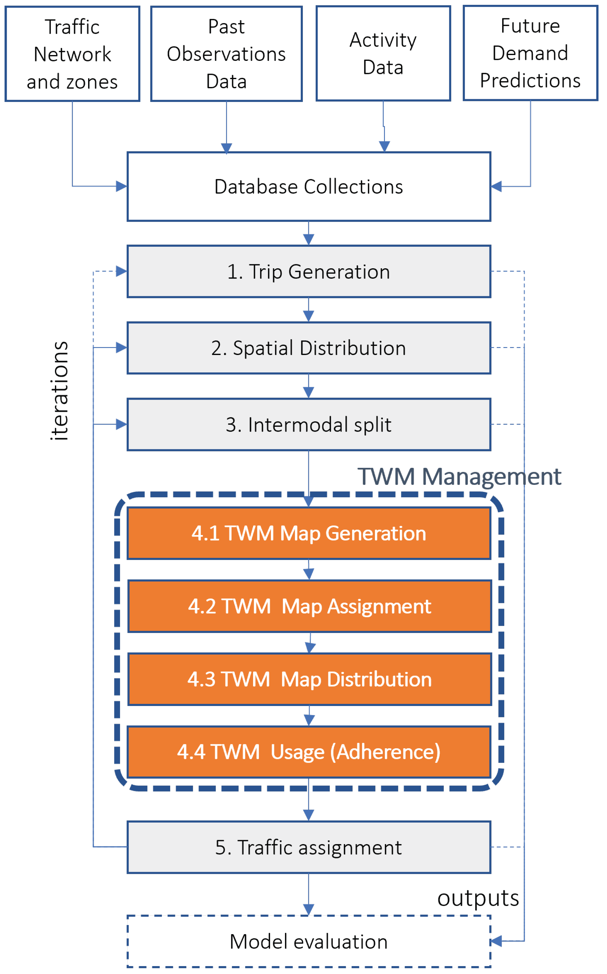
TWM can be seamlessly integrated into traffic planning systems mainly based on the trip-based demand model (TBM) or activity-based models (ABM) outlined by the USA Transportation Research Board [10]. The traffic network representation combines a physical view (how nodes and edges are connected) and a logical view (the operation and usage policies used) that is shared by all the users. This logic view may be operated between the inter-modal traffic split and the traffic assignment stage where the users are routed. Multiple views may be generated and distributed with differentiated traffic planning criteria so that the routing phase can be evaluated using them. For instance, electric cars may receive a different network than commercial distribution light-weight vehicles, scholar buses during certain times, or any other case. This approach also links with the activity-based models.

A new network management activities group would be required between the inter-modal split and the traffic assignment steps, as shown in Figure 1: TWM map generation, TWM map assignment policies to the routing agents, TWM map distribution strategies, and TWM usage models (utility models).

Emissions Models

Emissions estimation models can be mainly classified as microscopic or macroscopic (a complete review can be found in [24]). Microscopic models such as PHEM (Passenger Car and Heavy-Duty Emission Model) [25] allow a higher granularity based on speed changes, lane changes, and route and driving patterns. They also have a higher spatial and temporal resolution, identifying time-based hotspots. Their use is primarily suitable for small localized scenarios (intersections, roundabouts, and others), as they require higher computational effort and may be ineffective for large-scale scenarios.

On the other side, macroscopic estimation models such as HBEFA (Handbook on Emission Factors for Road Transport) [26] and the European Union “EMEP/EEA air pollutant emission inventory guidebook 2023” [27] implemented in COPERT [28] work at the aggregate level, considering average traffic characteristics. They have lower spatial and temporal resolution than microscopic simulations but require fewer resources. They are more suitable for significant areas, demand sizes, and temporal windows.

Traffic simulation environments such as SUMO [23] or AIMSUN [29] offer interfaces to integrate multiple emissions models.

The macroscopic emissions modeling is suitable for the static traffic assignment. Tsnakas et al. [30] have analyzed the accuracy of estimating traffic emissions in static traffic models, which may be inaccurate if the congestion situations are not correctly located. They suggest adding a post-processing with quasi-dynamic models. High-emission scenarios are strongly correlated with congestion situations.

3. TWM for Flow-Based Routing Strategies

This section introduces the network, demand, and TWM models. It also describes the mesoscopic emissions model used in this study and the sub-flow decomposition proposal for the TWM generation based on k-shortest paths (kSP-TWM) activity-based model (ABM).

Besides the models, this section covers the required details about OTV, LCTV, and UCTV algorithms for TWM map creation using k-shortest paths and for TWM optimal distribution.

3.1. Network and Routing Model

The urban network $\Theta$ is described by a graph $\Theta =G(N,E)$ formed by N nodes and E edges (links) $\left\{e\right\}$ connecting them. Considering the traffic flow $x_e$ that traverses an edge e, the vehicle cost of traversing an edge $c_e$ includes both the travel time $t_e\left(x_e\right)$ and the eventual tolls ${\tau }_e$ that could apply (1) [11].

$$c_e=t_e\left(x_e\right)+{\tau }_e$$

(1)

The edge travel time $t_e\left(x_e\right)$ depends on (a) edge properties (length $l_e$, max speed $s_e$,) and (b) edge occupation/capacity ratio, which depends on the road type. It is expressed by a volume-delay function $\Psi$ (VDF). The American Bureau of Public Roads (BPR) [31] has defined VDF models to reflect the impact of edge occupancy being (2) the most widely used, where $W_e$ is the link capacity [32], $x_e$ is the accumulated traffic flow traversing the edge e, and $\alpha$ and $\beta$ are predefined constants by [31] (typical values of $\alpha =0.15$ and $\beta =4.0$).

$$t_e\left(x_e\right)=\frac{l_e}{s_e}·{(1+\alpha \frac{x_e}{W_e})}^{\beta }$$

(2)

Traffic demand is composed of all the user mobility needs (vehicles $\left\{v_i\right\}$) expressed as origin/destination tuples (commodities, D) at the same time slots (O/D matrix). A traffic flow $x^d$ comprises the vehicles belonging to the same commodity $d$, moving from exact origin and destination. They may refer to network nodes, traffic area zones, or traffic centroids.

There are $P^d,(p_i^d\in P^d)$ feasible paths in a traffic network connecting an O/D commodity. Each path is expressed as an ordered sequence of consecutive edges connecting it with no loops. Each routing agent ${\upsilon }_a$ is responsible for selecting statically or dynamically the most convenient path $p_i^d$, which is called route $r_a$.

According to this, the traffic flow $x^d$ can be divided into sub-flows $\left\{x_i^d\right\}$ called path flows containing each one of the vehicles that have selected the same route $r_a$ (3):

$$x^d=\left\{x_i^d\right\},\forall v_a,v_b\in x_i^d,r_a=r_b$$

(3)

The traffic flow $x_e$ traversing an edge e is formed by the addition of traffic routed through it (4).

$$x_e=\sum x_i^d,\forall e\in \left\{p_i^d\right\}$$

(4)

The travel time $t_i^d$ over path $p_i^d$ is obtained by the aggregation of the travel time at all the traversed edges (5), as well as its generalized cost model $c_i^d$, which considers both the travel time and the possible tolls associated (6) [33].

$$t_i^d=\sum t_e\left(x_e\right),\forall e\in p_i^d$$

(5)

$$c_i^d=\sum c_e=\sum t_e\left(x_e\right)+\sum {\tau }_e,\forall e\in p_i^d$$

(6)

The route length $L_a$, number of traversed edges $E_a$, and number of traversed nodes $N_a$ are additional metrics associated with the route $r_a$.

3.2. Emissions Model

The European Union “EMEP/EEA air pollutant emission inventory guidebook 2023” [27] proposes three estimation methods that can be applied at the mesoscopic level, depending on the national statistics provided:

• Tier-1 method: aggregates individual emissions based on (a) fuel consumption of vehicle category and (b) fuel consumption-specific pollutant emission factor per fuel and category. The vehicle categories are passenger, light commercial, heavy-duty, and L-category vehicles. The fuels to be considered include petrol, diesel, LPG, and natural gas. It summarizes the tier-3 method.
• Tier-2 method: considers the fuel used by different vehicle categories, their technologies, and their emission standards and control legislation (Conventional, Euro-1, … Euro-6).
• Tier-3 method: considers mainly the operation conditions of the vehicles (hot, cold) and the type of roads used (urban, rural, highway). They are combined with the fuel chemical and energy properties to provide a detailed emissions model.

Our emissions evaluation model uses the tier-3 model, which proposes a generic Equation (7) for hot emissions that provides the emissions factor $E{f}_e^a$ in g/km for any of the pollutants 4 considering the individual vehicle $v^a$ driving at speed $s_e^a$ on a concrete road (edge e). Parameters $\left\{k_1,k_2,k_3,k_4,k_5,k_6,k_7,R{f}_1\right\}$ are publicly coded in the table RTV as $\left\{alfa,beta,gamma,delta,epsilon,zeta,eta\right\}$ columns [27], where the $R{f}_1$ is a reduction factor in the row.

$$E{f}_e^a\left(\rho \right)=\frac{k_1·{\left(s_e^a\right)}^2+k_2·s_e^a+k_3+\frac{k_4}{s_e^a}}{k_5·{\left(s_e^a\right)}^2+k_6·s_e^a+k_7}·(1-R{f}_1)$$

(7)

The driving mean speed $s_e^a$ is calculated from the maximum speed of the edge and the mean travel time in the edge once the STA has been calculated:

$$s_e^a=min(s_e,\frac{l_e}{t_e\left(x_e\right)})$$

(8)

According to this, the emissions ${\rho }_e^a$ for pollutant $\rho$ generated by a vehicle $v^a$ driving at speed $s_e^a$ in the edge e are:

$${\rho }_e^a=E{f}_e^a\left(\rho \right)·l_e$$

(9)

The function getEmissionsFactor (10) retrieves the $\left\{k_1,k_2,k_3,k_4,k_5,k_6,k_7,R{f}_1\right\}$ parameters from the vehicle properties, the emissions considered, the edge properties, and the edge operating conditions:

• Vehicle properties $v_{properties}$ include the category, fuel, segment, euro-standard, load, and technology.
• Pollutant $\rho$.
• Road (edge) properties $e_{properties}$ include the slope, min/max speed, and type (urban, rural, highway).
• Road (edge) operating conditions $e_{conds}$ describe the traffic status in the link: peak/off-peak status.

$$getEmissionsFactor:v_{properties},\rho ,e_{properties},e_{conds}\to \left\{k_1,\dots ,k_7,R{f}_1\right\}$$

(10)

Once the ${\rho }_e^a$ emissions per vehicle and edge are obtained, it is straightforward to obtain the total emissions per vehicle, per edge and per path flow, and also the total emissions in the traffic network.

It is also important to set when an edge should be considered in the “Urban Peak” status [27]. A 9 km/h limit will be considered, as any minor disturbance could stop the link completely. When the mean link speed after the assignment is below this threshold, we consider the edge as “Urban Peak”; otherwise, it will be in the “Urban Off-Peak”, “Rural”, or “Highway”.

3.3. Sub-Flow Decomposition on Emissions Categories

Activity-based traffic assignment models (ABM) [34] consider an individual’s utility functions and driving constraints. For our study, we consider emissions categories instead of these utility functions, so the vehicles are grouped fleets based on the emission parameters for specific routing policies using TWM.

Following the EU Tier-3 directives, the vehicles may be grouped into Q categories (or traffic groups) according to their emissions category, sub-type, fuel type, euro-standard, and operative age (usage). In our study, we will consider exclusively the fuel type, the parameter closest to the vehicle user. Adding new features is a straightforward process. Traffic flows $X=\left\{x^q\right\},\forall q\in Q$ are also classified depending on the emissions model.

Table 1. Traffic emissions sub-flow decomposition for 6 commodities and fuel types [4].

Commodity (O/D Pair)
Fuel		d1	d2	d3	d4	d5	d6
	Petrol	$x^{1,1}$	$x^{1,2}$	$x^{1,3}$	$x^{1,4}$	$x^{1,5}$	$x^{1,6}$
	Diesel	$x^{2,1}$	$x^{2,2}$	$x^{2,3}$	$x^{2,4}$	$x^{2,5}$	$x^{2,6}$
	CNG	$x^{3,1}$	$x^{3,2}$	$x^{3,3}$	$x^{3,4}$	$x^{3,5}$	$x^{3,6}$
	LPG	$x^{4,1}$	$x^{4,2}$	$x^{4,3}$	$x^{4,4}$	$x^{4,5}$	$x^{4,6}$
	Electric	$x^{4,1}$	$x^{4,2}$	$x^{4,3}$	$x^{4,4}$	$x^{4,5}$	$x^{4,6}$
	Hybrid	$x^{5,1}$	$x^{5,2}$	$x^{5,3}$	$x^{5,4}$	$x^{5,5}$	$x^{5,6}$
	Other	$x^{6,1}$	$x^{6,2}$	$x^{6,3}$	$x^{6,4}$	$x^{6,5}$	$x^{6,6}$

shows an example of traffic flow decomposition for six commodities and six fleets.

3.4. kSP-TWM Generation Strategies

A traffic weighted multi-map TWM $\left[{\mu }_m\right]$ is an M-dimensional set of different views of a traffic network $\Theta$. Each map ${\mu }_m$ is a complementary representation of the traffic network $\Theta$ (the m view) that is created using $\Pi$ functions (11). They receive as input the original network $\Theta$, the Q traffic group (fleet) constraints, and the time constraints (temporal rules) ${\Gamma }_m$. Temporal rules state the time validity constraints for each map, as they can be applied only for certain periods. $\left[{\beta }_e^m\right]$ represent the collection of specific edge weights designed for the TWM map m. TWM could be distributed as simple alternative network maps where some links have modified costs $\left[{\beta }_e^{*}\right]$ or internally used in the ITS as $\left[{\beta }_e^m\right]$ matrices.

$$\begin{array}{cc}\hfill \Pi & :\Theta ,Q,\left[{\Gamma }_m\right],\mathsf{\Phi }\to \left[{\mu }_m\right]\hfill \\ \hfill & {\mu }_m=\{\left[{\beta }_e^m\right],{\Gamma }_m\}\hfill \end{array}$$

(11)

TWM cardinal is a fundamental choice. In the flow-path approach for OTV/UCTV/LCTV, $numPF$ maps are generated depending on the number of commodities (F) and the number of kSP (K) used to route each one, as described in [9]. The TWM cardinality will be: $numPF=card\left(\left[{\mu }_m\right]\right)=F·K$. If we additionally consider the emissions grouping (Q) as described in the previous section, then the cardinality will be $numPF=card\left(\left[{\mu }_m\right]\right)=F·K·Q$.

TWM $\left[{\mu }_m\right]$ maps are created using $\Pi$ functions (11) that receive as input the original network $\Theta$, the Q traffic group (fleet) constraints, and the time constraints (temporal rules) ${\Gamma }_m$. Temporal rules state the time validity constraints for each map, as they can be applied only for certain periods. $\left[{\beta }_e^m\right]$ represent the collection of specific edge weights designed for the TWM map m.

A transformation function ${\rm Y}$ is applied to the weight of the ${\mu }_m$ map edges that are part of the kSP $r_i^d$ to obtain TWM maps that encourage using the different kSP obtained for each commodity. The ${{\rm Y}}_{Stretch}$ function (12) implements a weighted strategy, where each map ${\mu }_m$ uses a ${\alpha }_m$ scaling factor depending on a global scaling factor ${\alpha }^e$ and the relative cost influence (stretch) of the path flow $r_i^d$ over the total path flows $\left\{r_i^d\right\}$ available for the same flow. It is normalized using total travel-time $ff{c}_i^d$ under the free-flow conditions, which is the minimum route cost. $\left[{\beta }_e^{d,i}\right]$ represents the collection of edge weights for the TWM map created using the route $r_i^d$. ${\omega }_e$ represents the free-flow cost at the edge e.

$$\begin{array}{cc}\hfill {{\rm Y}}_{Stretch}& :\Theta ,r_i^d,\left[ff{c}_i^d\right],{\alpha }^e\to \left[{\beta }_e^{d,i}\right]=\left[{\omega }_e\right]·{\alpha }_m,\forall e\in \left\{r_i^d\right\}\hfill \\ \hfill & {\alpha }_m={\alpha }^e·\frac{min\left(ff{c}_i^d\right)}{ff{c}_m^d}\hfill \end{array}$$

(12)

Figure 2 shows an example of a 3-TWM generation for a basic traffic network with three kSP and ${\alpha }^e=0.5$ factor.

When the routing agent uses the TWM map ${\mu }_i^d$ based on the path flow $r_i^d$, the route costs are calculated with the new edge weights. The occupancy/capacity link-cost model described by (2) evolves to (13), also described as the edge volume-delay function $\Psi \left(x_e\right)$ using the TWM map.

$$t_e^{TWM}\left(x_e\right)={\beta }_e^{d,i}·{(1+\alpha \frac{x_e}{W_e})}^{\beta }$$

(13)

3.5. kSP-TWM Optimal Distribution Strategies

Once the TWM maps have been generated based on the kSP, the question to be solved is what will be their best allocation to achieve the system’s optimum, measured as the minimum mean travel time. Several optimization algorithms were described in [9] based on evolutionary approaches:

• Random Assignment (RA). It considers distributing randomly the TWM maps.
• Optimal Assignment of TWM (OTV), focused on obtaining the optimal TWM map-to-vehicle assignment from an individual perspective. The objective is to minimize travel time by creating an optimal map assignment. The optimization process involves calculating the index $n\in \left[1\dots K\right]$ to determine the application of the $\left[{\mu }_i^d\right]$ from the TWM for each vehicle, as illustrated in Figure 3. The genetic algorithm (GA) function generates a chromosome ${\aleph }_0$ consisting of the indices representing the corresponding map in the TWM, which are directly assigned to the vehicles. The OTV fitness function is shown in Algorithm 1. It receives the chromosome ${\aleph }_0$ to evaluate, the VDF function $\Psi$, the physical network map ${\mu }_0$, the traffic flows $\left\{x_i^d\right\}$, the path flows $\left\{r_i^d\right\}$, and the TWM $\left[{\mu }_i\right]$. OTV presents some major issues: The chromosome size in OTV is directly tied to the number of vehicles in the network, requiring a substantial amount of computational resources. Even in small traffic scenarios, it can be unaffordable. Secondly, this approach may not accurately reflect traffic planning, as it relies on specific trips, thus losing the mesoscopic perspective of routing traffic demand as flows.
• Optimal Assignment of TWM per Path Flow with Linear Constraints (LCTV): It overrides the OTV complexity, assigning the TWM on a per-flow basis. All the vehicles belonging to that flow receive the same TWM map. The optimization problem deals with the number of vehicles to be assigned to each path flow to obtain the minimum mean travel time. The problem contains linear constraints related to flow conservation and normalization.
• Unconstrained Optimal Assignment of TWM per Path Flow (UCTV): The optimal assignment can be solved by removing the linear constraints from the GA engine and applying them to the optimization results. This approach expands the range of the genetic solutions to be considered and accelerates GA convergence and computing effort.

Algorithm 1 OTV fitness function

Require: traffic assignment chromosome ${\aleph }_0$, traffic network $\Theta$, TWM map $\left[{\mu }_i^d\right]$, vehicles $〈v_a〉$, flows $〈x_i^d〉$, path flows $〈r_i^d〉$, volume-delay function $\Psi$ Ensure: mean total travel time $mtts$   1: for all (v in $〈v_a〉$) do   2:    $v.map\leftarrow int\left({\aleph }_0\left(v\right)\right)$ {direct map assignment}   3: end for   4: $〈p_i^d〉\leftarrow staticAssignment(\Theta ,〈v_a〉,〈x_i^d〉,\left[{\mu }_i^d\right],\Psi )$   5: $mtts\leftarrow computeMTTS({\mu }_i,〈p_i^d〉,\Psi ,{\Psi }_{args})$

The LCTV/UCTV strategy is shown in Figure 4. Each sub-flow $x_i^d$ is assigned a fixed TWM map ${\mu }_i^d$. The challenge now lies in solving the number of vehicles assigned to each sub-flow, that is, how many vehicles will use each ${\mu }_i^d$ efficiently. The distribution is determined as a percentage of the traffic for every commodity d. Consequently, each vehicle will be assigned the appropriate path flow map. The GA function generates the chromosome ${\aleph }_1$ with a $numPF$ size. Each value represents the percentage of vehicles from each flow allocated to a particular sub-flow $x_i^d$. Two constraints are applied to ensure the validity of the chromosome. Firstly, $[0\dots 1]$ normalization is enforced. Secondly, flow conservation is maintained, which means that the sum of all vehicle percentages belonging to the same flow must equal 1. Both constraints are directly incorporated into the GA algorithm.

Linear constraints applied to the GA problem-solving process create a bias in the electable population: although better individuals are chosen, less diversity is used to search for alternative solutions. As the experimental results show, this elimination of individuals evaluates the algorithm longer and leads to worse results. In addition, the unconstrained solver UCTV applies the normalization step at the end of the process to the resulting values to compute the corresponding TWM distribution in Algorithm 2.

Algorithm 2 LCTV/UCTV fitness function

Require: traffic assignment chromosome ${\aleph }_0$, traffic network $\Theta$, TWM map $\left[{\mu }_i^d\right]$, vehicles $〈v_a〉$, flows $〈x_i^d〉$, path flows $〈r_i^d〉$, volume-delay function $\Psi$ Ensure: mean total travel time $mtts$   1: for all (x in $〈x_i^d〉$) do {iterate over the flows}   2:    $〈v^d〉\leftarrow 〈v_a〉,v_a.flow==x)$ {flow population}   3:    $nv\leftarrow count(〈v^d〉$) {number of flow vehicles}   4:    $np\leftarrow count\left(〈x_i^d〉\right)$ {number of path flows to be assigned}   5:    $〈p{c}_i〉\leftarrow pop({\aleph }_1,np)$ {extract np percents from ${\aleph }_1$}   6:    $〈p{c}_i〉\leftarrow normalize\left(〈p{c}_i〉\right)·nv$ {vehicle counts for each assignment}   7:    $〈mapIdx〉\leftarrow createMapIndexes(〈p{c}_i〉,x$)   8:    for all v in $〈v^d〉$) do   9:      $v.map\leftarrow mapIdx\left(v\right)$   10:   end for   11: end for   12: $〈p_i^d〉\leftarrow staticAssignment(\Theta ,〈v_a〉,〈x_i^d〉,\left[{\mu }_i^d\right],\Psi )$   13: $mtts\leftarrow computeMTTS({\mu }_i,〈p_i^d〉,\Psi ,{\Psi }_{args})$

The mean travel time evaluation procedure $computeMTTS$ (14) is applied. It evaluates the MTTS for a certain traffic flow (trips) $\left\{p_i^d\right\}$ over a network view ${\mu }_i$, using a certain volume-delay function $\Psi$ (VDF) [11] with its specific VDF arguments ${\Psi }_{args}$. The function considers a network loaded with the routed flow trips and computes the mean travel time of the vehicles, considering the specific volume-delay function. The VDF is evaluated at each edge based on the number of vehicles that are routed through it. The network description is based on the edge weights described by the specific TWM map ${\mu }_i$.

$$\begin{array}{cc}\hfill & computeMTTS:{\mu }_i,\left\{p_i^d\right\},\Psi ,{\Psi }_{args}\to mtts\hfill \end{array}$$

(14)

$$\begin{array}{cc}\hfill & x_e\leftarrow count\left(e\right),\forall e\in \left\{p_i^d\right\}\hfill \end{array}$$

(15)

$$\begin{array}{cc}\hfill & mtts\leftarrow mean(\Psi ({\mu }_i\left({\beta }_e^{d,i}\right),x_e,{\mu }_i\left(W_e\right),{\Psi }_{args}),\forall e\in \left\{p_i^d\right\}\hfill \end{array}$$

(16)

$\Psi \left(x_e\right)$ uses the volume-delay function using the TWM map described in (13).

As an example, for TWM assignment, let us consider the traffic flows $x_1=500$, $x_2=500$, and $x_3=500$ vehicles, using TWM based on 3-Shortest Paths (3SP). In this scenario, the optimization chromosome for individual routing is reduced from 1500 genes ($x_1+x_2+x_3$,) to the path flow chromosome with 9 genes ($3flows·3ksp$).

If the chromosome ${\aleph }_1\left[\left(0.6,0.25,0.15\right),\left(0.5,0.2,0.3\right),\left(0.3,0.25,0.45\right)\right]$ is returned by the GA, then the path flows assigned will be $\left[\left[300,125,75\right],\left[250,100,150\right],\left[150,125,225\right]\right]$, for instance, $x_1^1=x_1·{\aleph }_1(1,1)=500·0.6=300$, $x_2^1=x_1·{\aleph }_1(1,2)=500·0.25=125$, and so on. Each path flow will be routed accordingly with the corresponding TWM map assignment $\left[{\mu }_1^1,{\mu }_2^1,{\mu }_3^1,{\mu }_1^2,{\mu }_2^2,{\mu }_3^2,{\mu }_1^3,{\mu }_2^3,{\mu }_3^3\right]$.

4. Experimental Results

The experimental scenarios are referenced to the original GRID64 and traffic demands described in [9,21]. The emissions models are added, and the new sub-flows corresponding to the differential routing for each vehicle fuel category are included.

On the emissions side, other contextual factors such as weather conditions, day of the week, seasonality of demand, and similar variants have not been taken into account, as we are considering a traffic snapshot that is studied under the different traffic assignment strategies that have identifical context properties. Our objective is focused on comparing the emissions produced in the different routing strategies using TWM. Also, average vehicle occupancy and load values and a neutral slope in the route links have been considered in the emissions models.

4.1. Materials and Methods

The experiments were developed using Matlab R23A on a Windows 11 system with an iCore7 2.10 GHz processor and 64 GB RAM.

The genetic algorithms utilized Matlab’s global optimization toolbox [35].

The resulting TWM maps are dumped in data files compatible with SUMO 1.19 [23].

The solutions use a plugin developed for TWM management through the TRACI interface at SUMO.

Each TWM allocation strategy involving a stochastic process was repeated 100 times for the GA execution and the random population adherence to achieve the necessary confidence intervals in the results presented.

4.2. Synthetic Urban Scenario Grid-64

Following the previous reference works, the GRID64 network is used. Figure 5 shows the network formed by an 8 × 8-node grid network with bidirectional edges. The node names and edge lengths are shown, and traffic demand sources are colored (red for sources, yellow for destination). Design criteria for the scenario are taken from the Ortuzar–Willumsen scenario described in [11,36], where more extensive reference networks are required for generating a relevant number of kSP.

All the edges are featured as “Urban Off-Peak”, considering a 9 km/h lower threshold for the “Urban Peak” status.

4.3. Characterization of Traffic Demand

Six commodities are defined for the traffic demand, comprising three traffic sources at $(N_{73},N_{75},N_{77})$ and two traffic sinks at $(N_{23},N_{26})$, described in

Table 2. GRID64 O/D Matrix.

Source/Destination	${\mathit{N}}_{73}$	${\mathit{N}}_{75}$	${\mathit{N}}_{77}$
$N_{23}$	1000	500	1000
$N_{26}$	500	1000	500

, where traffic volumes are also included. The STA experiment covers a total of 4500 vehicles.

These vehicles must be classified according to their emissions features in terms of category, type, emissions for euro-standards, and fuel type.

Table 3. Demand distribution for category, fuel type and emissions euro-standards.

Category	Euro-Standard	CNG	Diesel	Electric	Hybrid	LPG	Other	Petrol	Total
Buses	Conventional		2						2
	Euro 3		1						1
	Euro 4		2						2
	Euro 6		2						2
Total Buses			7						7
Heavy-Duty Trucks	Conventional		112					8	120
	Euro 3		58					1	59
	Euro 4		32					1	33
	Euro 5		30					2	32
	Euro 6		52					1	53
Total Heavy-Duty Trucks			284					13	297
L-Category	Conventional							529	529
	Euro 6			8	6				14
Total L-Category				8	6			529	543
Light Commercial Vehicles	Conventional		83					28	111
	Euro 3		44					2	46
	Euro 4		47					1	48
	Euro 5		36					3	39
	Euro 6	1	91	2	2	1		9	106
Total Light Commercial Vehicles		1	301	2	2	1		43	350
Passenger Cars	Conventional		264				1	492	757
	Euro 3		311					98	409
	Euro 4		332					180	512
	Euro 5	2	362			1		177	542
	Euro 6	19	483	14	19	14		534	1083
Total Passenger Cars		21	1752	14	19	15	1	1481	3303
Total general		22	2344	24	27	16	1	2066	4500

describes the vehicle volumes corresponding to each section and their cumulative values. The distribution follows a homogeneous structure to the traffic vehicle composition in Spain, as published by the Spanish regulator DGT [37]. The yearly report contains the vehicle categories and standards decomposition, following the European directives.

Several experiments are conducted over the same traffic scenario (network and traffic demand) using different configurations of kSP-based TWM to evaluate the following indicators:

• Total travel time after assignment (data in

  Table 4. Experimental data for Grid64: total travel time (h).

  	0-Free-Flow	0-UE_CUM	0-UE_MSA	2-KSP Random	2-TWM Random	2-TWM UCTV	3-KSP Random	3-TWM Random	3-TWM UCTV	5-KSP Random	5-TWM Random	5-TWM UCTV	7-KSP Random	7-TWM Random	7-TWM UCTV
  mean	56	139	128	7894	1997	1947	1119	256	243	269	156	156	251	155	147
  median	56	139	128	8250	1997	1997	1145	278	254	271	157	163	253	156	154
  Low-95	56	139	128	7544	1779	1800	1050	226	227	253	139	146	236	138	137
  Up-95	56	139	128	8243	2216	2094	1187	287	259	284	173	166	265	172	157

  ).
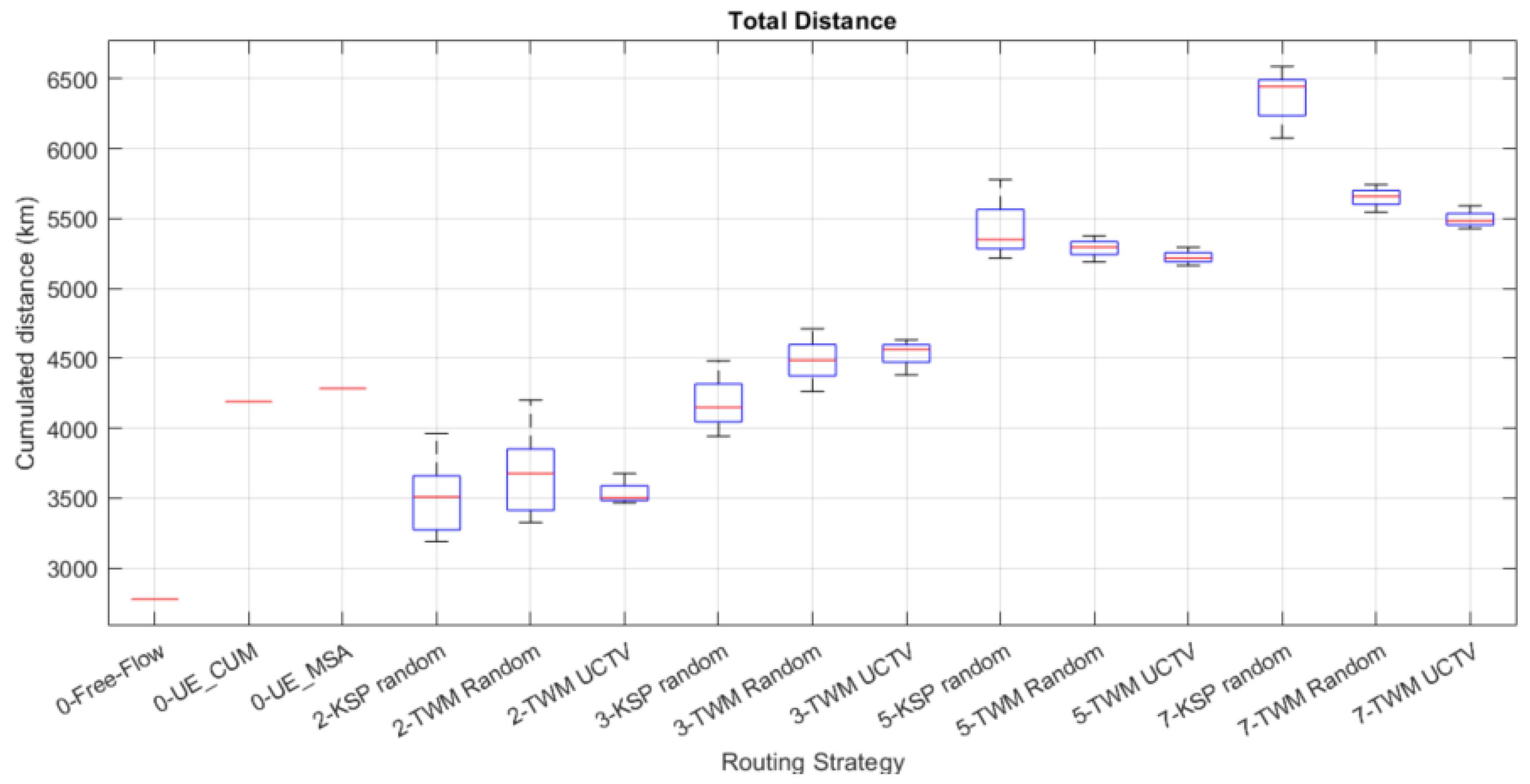
• Total distance followed by the vehicles (data in

  Table 5. Experimental data for Grid64: total distance (${10}^3$ km).

  	0-Free-Flow	0-UE_CUM	0-UE_MSA	2-KSP Random	2-TWM Random	2-TWM UCTV	3-KSP Random	3-TWM Random	3-TWM UCTV	5-KSP Random	5-TWM Random	5-TWM UCTV	7-KSP Random	7-TWM Random	7-TWM UCTV
  mean	2.78	4.19	4.29	3.49	3.65	3.53	4.19	4.49	4.55	5.42	5.29	5.22	6.38	5.66	5492
  median	2.78	4.19	4.29	3.51	3.68	3.50	4.15	4.49	4.56	5.35	5.30	5.22	6.44	5.66	5481
  Low-95	2.78	4.19	4.29	3.99	3.54	3.51	4.13	4.43	4.52	5.36	5.27	5.21	6.31	5.63	5475
  Up-95	2.78	4.19	4.29	3.59	3.76	3.56	4.25	4.55	4.58	5.49	5.32	5.24	6.44	5.68	5510

  ).
• Number of routes that the routing agents selected. This parameter must be distinguished from the number of path-flows, as the latter is a consequence of the path-flow routing algorithm, which sets its value to F·K (number of flows per number of kSP).
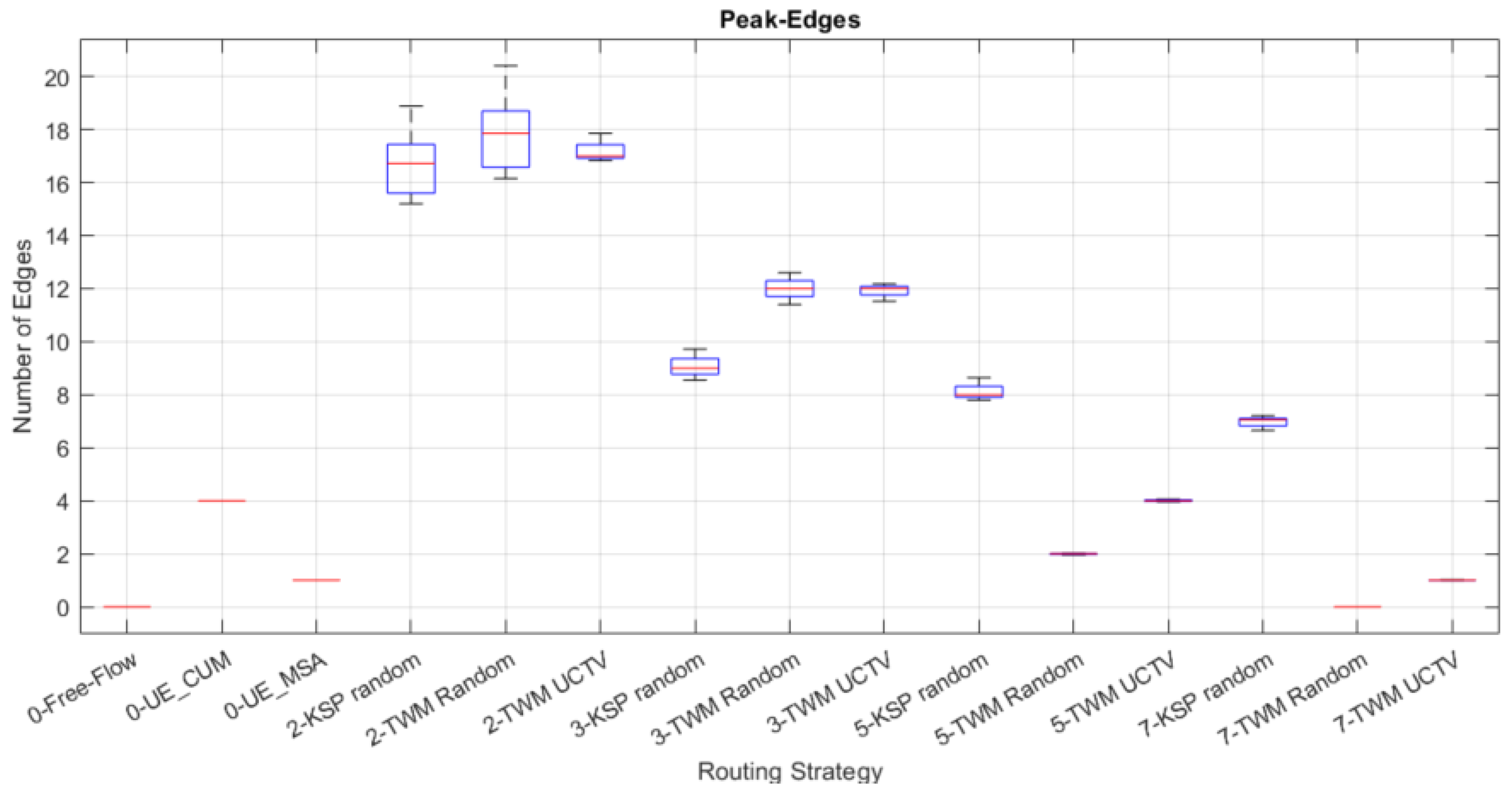
• Number of edges that were found in the “Urban Peak” situation (data in

  Table 6. Experimental data for Grid64: peak edges (count).

  	0-Free-Flow	0-UE_CUM	0-UE_MSA	2-KSP Rndom	2-TWM Random	2-TWM UCTV	3-KSP Random	3-TWM Random	3-TWM UCTV	5-KSP Random	5-TWM Random	5-TWM UCTV	7-KSP Random	7-TWM Random	7-TWM UCTV
  mean	0	4	1	17	18	17	9	12	12	8	2	4	7	0	1
  median	0	4	1	17	18	17	9	12	12	8	2	4	7	0	1
  Low-95	0	4	1	16	17	17	9	12	12	8	2	4	7	0	1
  Up-95	0	4	1	17	18	17	9	12	12	8	2	4	7	0	1

  ).
• Total length of the “Urban Peak” edges (data in

  Table 7. Experimental data for Grid64: peak edges total distance (km).

  	0-Free-Flow	0-UE_CUM	0-UE_MSA	2-KSP Random	2-TWM Random	2-TWM UCTV	3-KSP Random	3-TWM Random	3-TWM UCTV	5-KSP Random	5-TWM Random	5-TWM UCTV	7-KSP Random	7-TWM Random	7-TWM UCTV
  mean	0	250	69	1297	1650	1568	643	726	719	507	111	236	443	0	55
  median	0	250	69	1298	1652	1555	625	726	722	500	111	236	447	0	55
  Low-95	0	250	69	1253	1594	1557	615	706	715	501	111	236	438	0	55
  Up-95	0	250	69	1341	1707	1580	672	746	724	513	111	237	447	0	55

  ).
• Volume of hot emissions (in kg): CO, NOx, VOC, and PM will be considered (data in

  Table 8. Experimental data for Grid64: hot emissions CO (kg).

  	0-Free-Flow	0-UE_CUM	0-UE_MSA	2-KSP Random	2-TWM Random	2-TWM UCTV	3-KSP Random	3-TWM Random	3-TWM UCTV	5-KSP Random	5-TWM Random	5-TWM UCTV	7-KSP Random	7-TWM Random	7-TWM UCTV
  mean	14.44	27.48	26.96	2380.37	587.93	558.72	271.92	29.97	33.62	85.55	33.23	33.79	17.69	34.15	33.38
  median	14.44	27.48	26.96	2382.92	588.56	553.94	264.12	29.96	33.76	84.40	33.24	33.75	17.88	34.16	33.32
  Low-95	14.44	27.48	26.96	2298.92	567.81	554.76	259.81	29.13	33.41	84.49	33.10	33.70	17.52	34.02	33.28
  Up-95	14.44	27.48	26.96	2461.83	608.05	562.68	284.03	30.81	33.84	86.60	33.36	33.88	17.87	34.29	33.49

  ,

  Table 9. Experimental data for Grid64: hot emissions NOx (kg).

  	0-Free-Flow	0-UE_CUM	0-UE_MSA	2-KSP Random	2-TWM Random	2-TWM UCTV	3-KSP Random	3-TWM Random	3-TWM UCTV	5-KSP Random	5-TWM Random	5-TWM UCTV	7-KSP Random	7-TWM Random	7-TWM UCTV
  mean	2.34	3.89	3.90	37.00	11.76	11.17	8.56	4.74	4.92	5.67	4.91	4.75	6.09	5.01	5.09
  median	2.34	3.89	3.90	37.04	11.77	11.08	8.32	4.74	4.94	5.59	4.91	4.75	6.16	5.01	5.08
  Low-95	2.34	3.89	3.90	35.73	11.35	11.09	8.18	4.61	4.89	5.60	4.89	4.74	6.03	4.99	5.07
  Up-95	2.34	3.89	3.90	38.26	12.16	11.25	8.95	4.88	4.95	5.74	4.93	4.77	6.15	5.03	5.11

  ,

  Table 10. Experimental data for Grid64: hot emissions VOC (kg).

  	0-Free-Flow	0-UE_CUM	0-UE_MSA	2-KSP Random	2-TWM Random	2-TWM UCTV	3-KSP Random	3-TWM Random	3-TWM UCTV	5-KSP Random	5-TWM Random	5-TWM UCTV	7-KSP Random	7-TWM Random	7-TWM UCTV
  mean	3.29	7.16	4.75	6.38	5.15	4.87	7.80	6.07	5.43	8.00	6.89	6.37	7.76	6.54	5.60
  median	3.29	7.16	4.75	6.39	5.13	4.82	7.68	6.07	5.46	7.90	6.90	6.36	7.84	6.54	5.59
  Low-95	3.29	7.16	4.75	6.17	4.99	4.83	7.62	6.02	5.40	7.90	6.87	6.35	7.68	6.52	5.59
  Up-95	3.29	7.16	4.75	6.60	5.31	4.90	7.98	6.12	5.47	8.10	6.92	6.38	7.84	6.57	5.62

  and

  Table 11. Experimental data for Grid64: hot emissions PM (kg).

  	0-Free-Flow	0-UE_CUM	0-UE_MSA	2-KSP Random	2-TWM Random	2-TWM UCTV	3-KSP Random	3-TWM Random	3-TWM UCTV	5-KSP Random	5-TWM Random	5-TWM UCTV	7-KSP Random	7-TWM Random	7-TWM UCTV
  mean	0.50	0.89	0.89	0.78	1.54	1.45	1.13	1.10	1.11	1.28	1.08	1.11	1.40	1.16	1.13
  median	0.50	0.89	0.89	0.78	1.53	1.44	1.12	1.10	1.12	1.27	1.08	1.11	1.42	1.16	1.12
  Low-95	0.50	0.89	0.89	0.75	1.49	1.44	1.11	1.09	1.11	1.27	1.08	1.10	1.39	1.16	1.12
  Up-95	0.50	0.89	0.89	0.80	1.59	1.46	1.16	1.11	1.12	1.30	1.09	1.11	1.42	1.16	1.13

  ).

Different path flows are generated for the TWM maps using kSP values of {2,3,5,7}, corresponding to {12,18,30,42} path flows, respectively.

Different strategies for static traffic assignment are used to make a differential comparison. Except for the free-flow approach, which provides the lower traffic bound, all of them use the BPR VDF function described in (2), considering the links occupation after the traffic assignment phase.

• UE-CAM (cumulative assignment method) and UE-MSA (successive averages method), as they approximate the equilibrium situation to solve the TAP [11]. They do not propose an implementation for ITS, but provide an estimation for the TAP, which is used to compare how far the TWM solutions proposed are.
• The unrealistic random kSP direct selection from the routing agents. It assumes hypothetically that the drivers would choose a k-shortest path in a random way, without having or considering prior knowledge or the network status. Drivers do not use TWM in this case.
• TWM random assignment, that is, when the TWM based on path-flows is generated, they can be randomly assigned to the routing agents instead of creating an optimal delivery with LCTV or UCTV.
• TWM optimally assigned to the routing agents with the UCTV algorithm.
• Other mechanisms that provide upper bounds for static traffic assignments, such as all-or-nothing or free-flow, have not been included in the study, as their solutions are far away from those close to the equilibrium situations, distorting the quantitative results. We preferred to exclude them.

We use for the experiments the UCTV map allocation strategy, as it allows a reduction in computing complexity without losing accuracy, as was shown in our previous work [9].

The experiments have been repeated multiple times (20) to obtain consistent statistical results, which are covered in Table 4, Table 5, Table 6, Table 7, Table 8, Table 9, Table 10 and Table 11. They reflect the mean values, the median, and the confidence intervals corresponding to the 0.95 level, assuming a normal distribution of the values obtained, as there are enough experiment repetitions configured. These data are illustrated in Figure 6, Figure 7, Figure 8, Figure 9, Figure 10, Figure 11, Figure 12 and Figure 13, which reflect in box-plot diagrams the data dispersion showing the max and min values obtained, the median, and the 25 and 75 percent boxes for value distributions.

5. Discussion

Figure 6, Figure 7, Figure 8, Figure 9, Figure 10, Figure 11, Figure 12 and Figure 13 reflect the statistical results obtained for each strategy and number of kSP used; for instance, “5-TWM-UCTV” means that a 5-shortest path has been used.

UE-CAM and UE-MSA have no data dispersion, as they provide the equilibrium baseline for the TAP estimation to compare the rest of strategies. Our target strategy is the TWM-UCTV approach with k-shortest paths, whose optimal map distribution to the traffic flows is compared to the theoretical random strategies offered by the random usage of kSP and the random TWM assignment, which use a uniform data distribution for the drivers that would make them select non-optimal routes. The optimal TWM distribution has also some random behavior, as the solution search algorithm is based on genetic properties such as mutation, crossover, and selection.

The discussion analyzes all the variables studied in the paper.

5.1. Differential Routing, Travel Time, and Total Distance

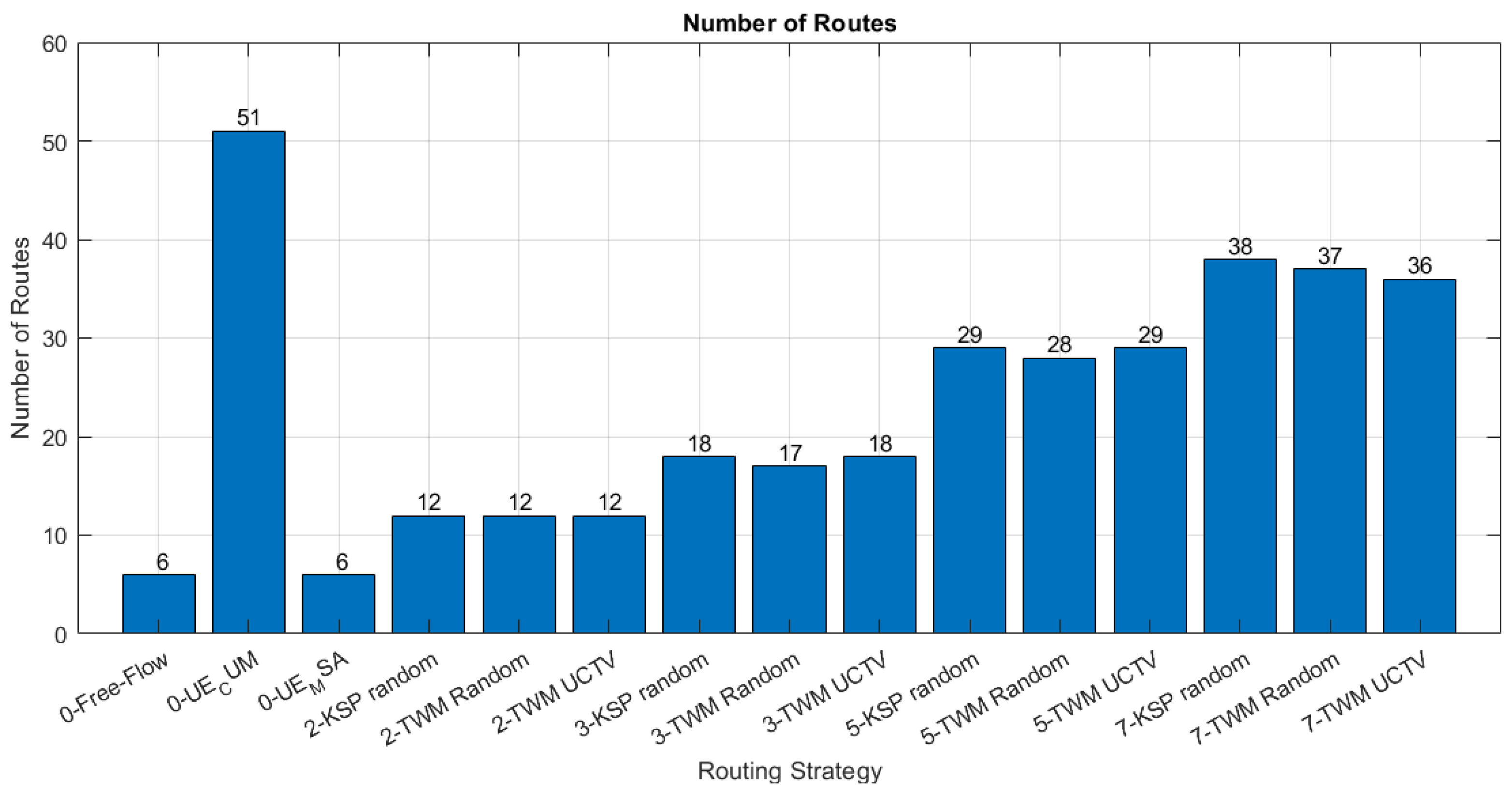
The number of routes used by the routing agents for the different strategies is shown in Figure 14. Free-Flow traffic estimation uses a single shortest-path routing for each traffic flow -6-, whilst UE_CAM and UE_MSA are just mathematical models to estimate edge occupations for the equilibrium considering the travel time; their routing depends on the calculus algorithm and is only relevant for the travel time estimation.

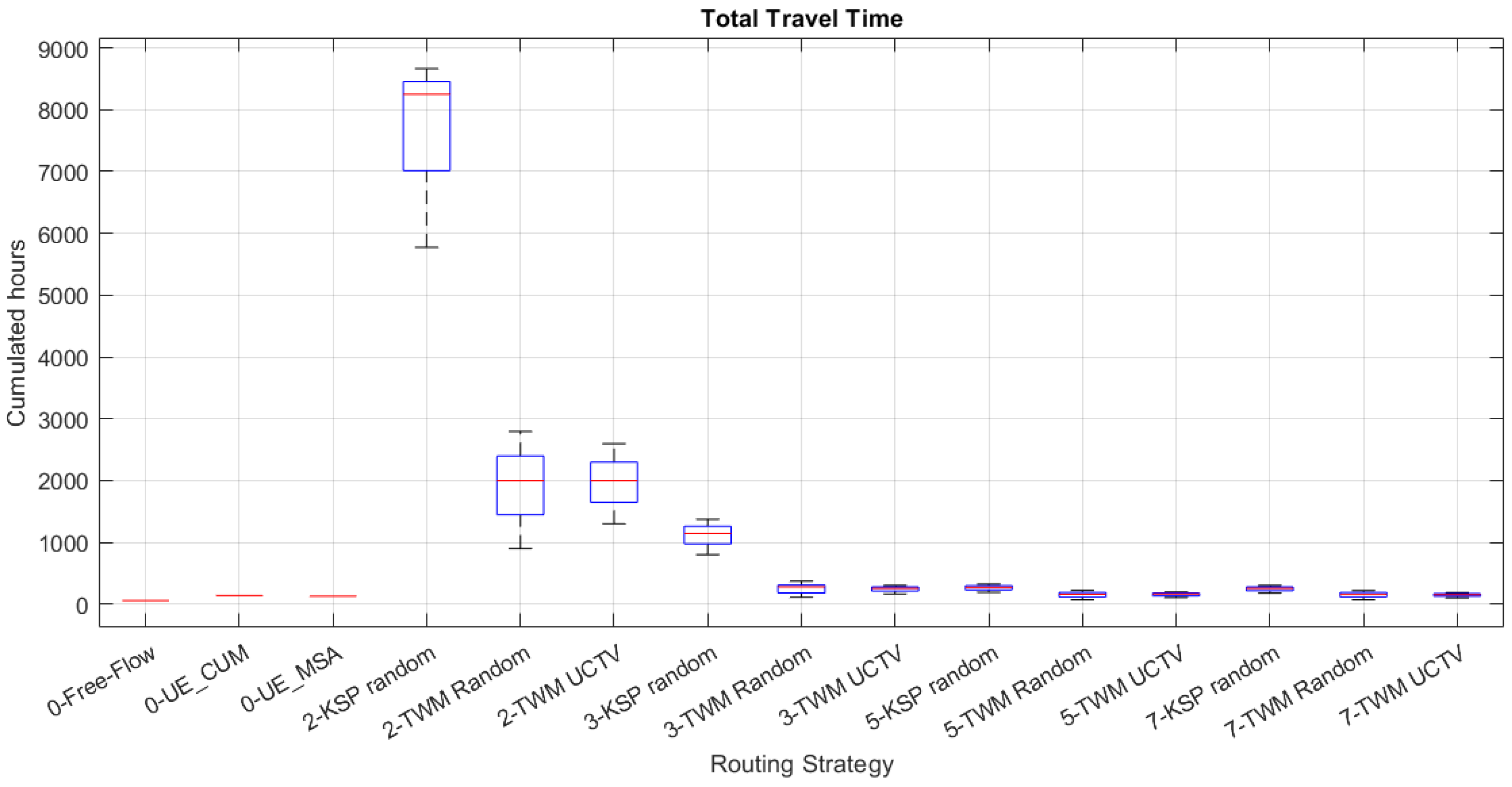
As expected, the gradual addition of new kSPs leads to a larger number of TWM maps being generated and distributed to drivers, thus inducing the selection of new routes based on link occupancy and new costs received. The use of 3-SP leads to the use of [17–18] routes, and the use of 5-SP or 7-SP increases to [28–29] and [36–38] routes, respectively. The diversity of routes also leads to a better travel time (Figure 6), which quickly approaches the expected equilibrium values and cannot be improved further. In our scenario, 3-SP are sufficient to reach this lower bound, and adding more alternative routes hardly improves the travel time. Even TWM created with 2-SP per traffic flow greatly improves travel time as a bare routing strategy.

However, when considering the total distance traveled by the vehicles, we can observe in Figure 7 that, despite having a similar travel time in many cases, the routes differ greatly in the distance as alternative roads with different lengths are included.

5.2. Congestion (Peak Edges)

It is not sufficient to consider the total travel time and distance traveled, but also the congested state of the links, which is identified when their average speed exceeds the defined lower threshold. Figure 8 describes the number of congested links. The VDF cost function evaluates a much higher value on these congested links, which causes the traffic assignment to select alternative paths. The diversity of routes also favors a reduction in the number of congested links, as we can see in Figure 8, so that by increasing the number of TWM maps from 3-SP to 5-SP the volume of peak links is reduced by almost half. The optimal TWM distribution is relevant to reduce the number of peak edges.

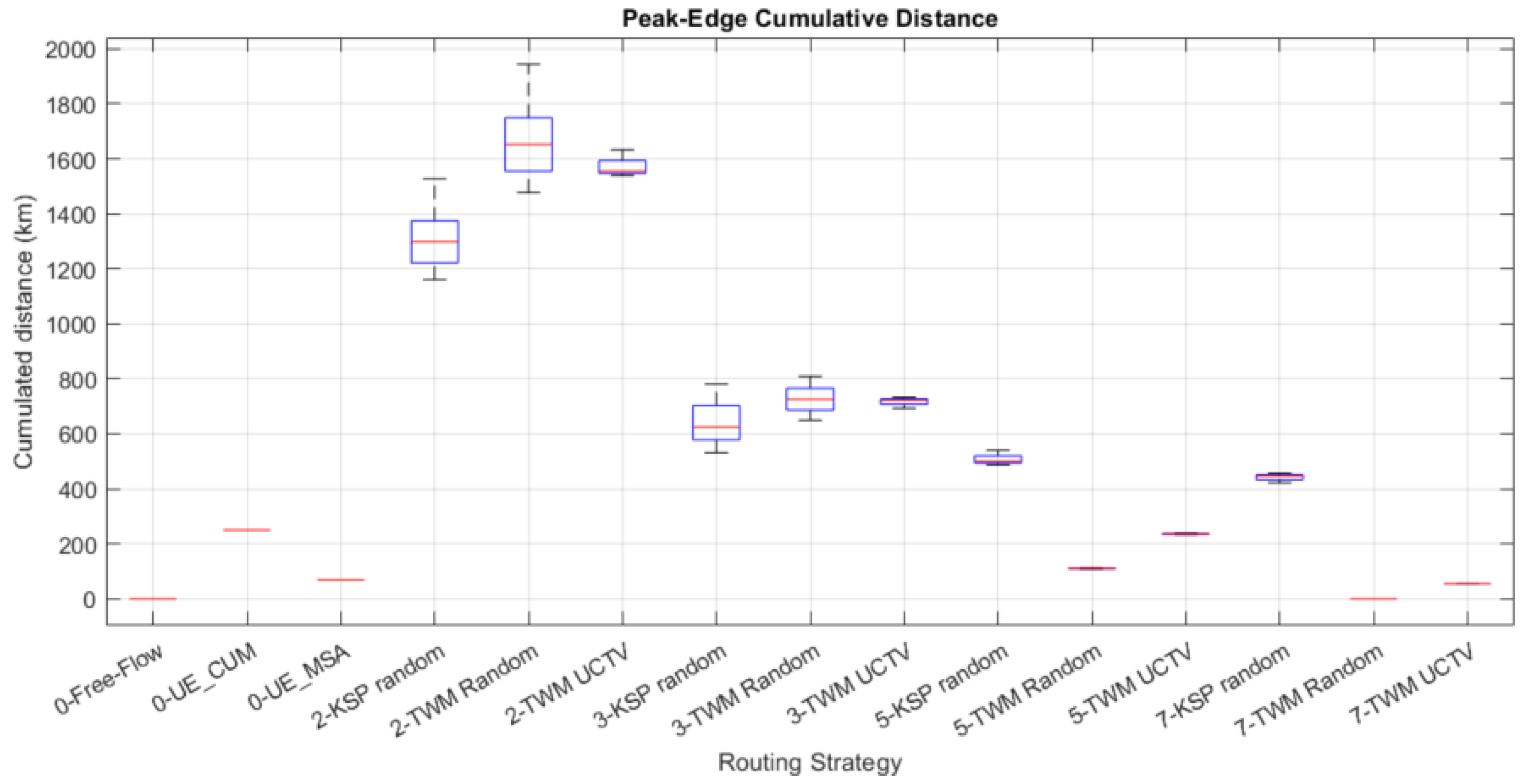
The emissions model also penalizes these congested links, applying the peak penalty factor. The congested path distance is also relevant, as the emissions rate also depends on the traveled distance under this traffic conditions. Figure 9 shows the cumulative travel distance under peak conditions for the different use cases.

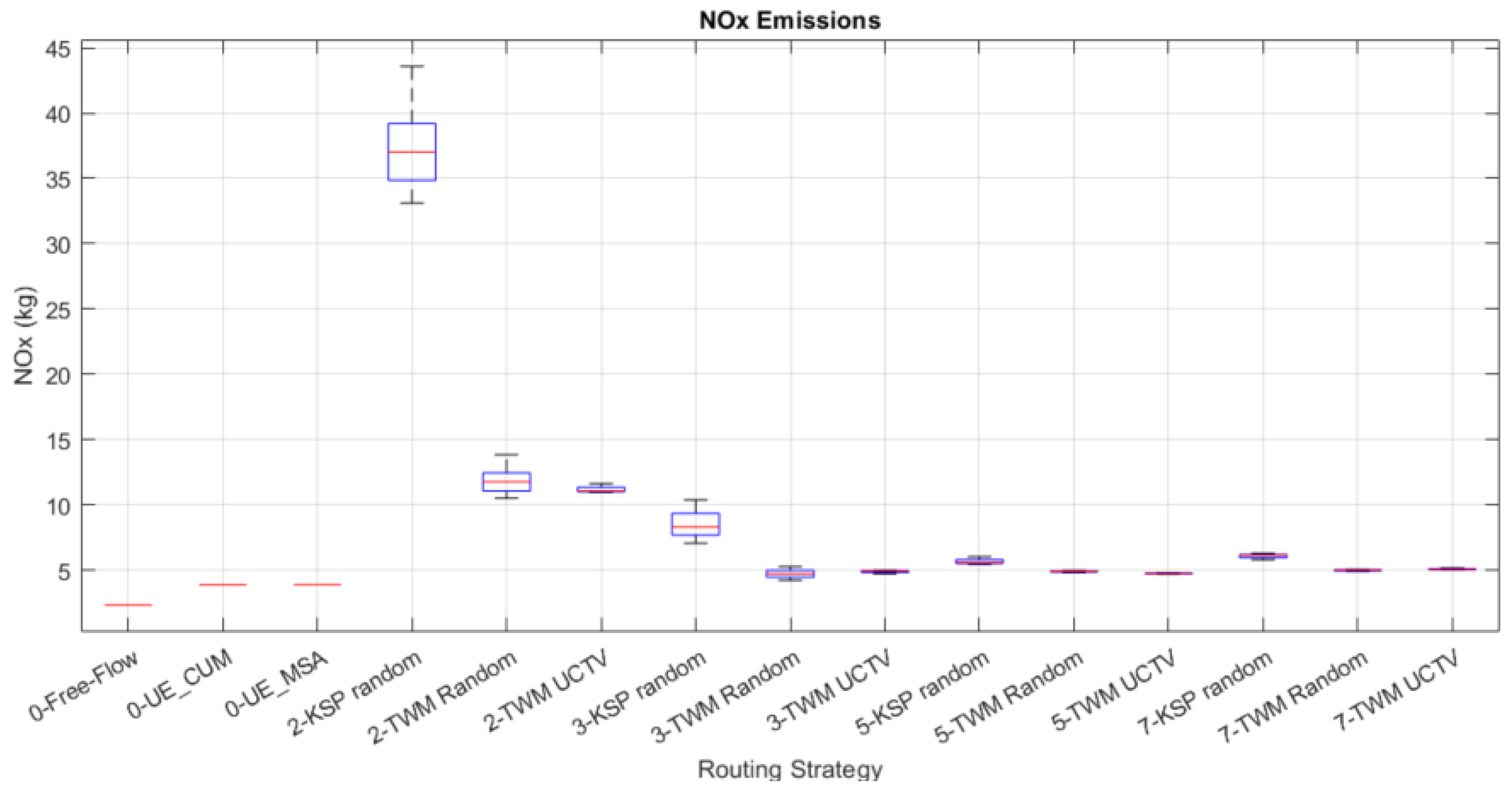
5.3. Hot Emissions

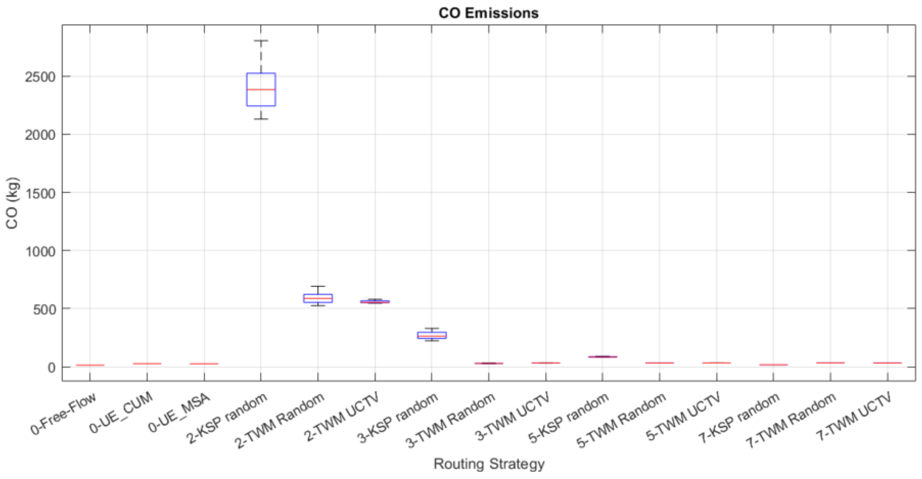
Consistent with the different traffic assignment strategies, the evolution of the hot emission models can be seen in Figure 10, Figure 11, Figure 12 and Figure 13. The hot emissions evaluation function described in (10) retrieves the parameters $\left\{k_1,k_2,k_3,k_4,k_5,k_6,k_7,R{f}_1\right\}$, which depend on the vehicle type, road conditions, and the peak/non-peak state, as set out in the EU Tier-3 hot emissions model [4]. These parameters are specific to each vehicle type at each edge condition and are used to assess the individual contribution per edge by applying the average speed and edge length.

CO and NOx are aligned with the travel time. As the travel time decreases due to the diversity of paths generated for the vehicles with the TWM maps, the model’s CO and NOx emission estimates decrease at the same rate, stabilizing quickly on the expected equilibrium values baseline (UE_CUM, UE_MSA). The feasible ways to reduce them would be modifying the intermodality of travel or vehicle mix or implementing low-emission zones (LEZs).

In the case of particle emissions, calibrated emission models reflect a strong correlation with the number and total length of congested edges, as well as the total distance traveled by vehicles. By offering vehicles greater route diversity, they may select longer routes than the merely optimal shortest path; however, their lower congestion and higher speed on their route will cause their emissions to become stable. The length of traveled trips affects particle emissions, which stabilize at 22% over the equilibrium expected baseline. They are mostly affected by the congestion and the randomness in the TWM allocation, as shown in Figure 12 and Figure 13. Optimal TWM distribution is a key factor for emissions reduction.

6. Conclusions

This paper extends the algorithm details outlined in [9] and demonstrates the potential for reducing total travel time within a traffic network by employing ad hoc generated TWM maps. These maps encourage the selective utilization of k-shortest paths for traffic flows, with total travel time assessed through static traffic assignment. TWM maps are crafted based on optimal kSP routes under free-flow conditions for each flow in the network. A routing agent will receive a specifically designed TWM map for its routing decisions, and it will tend to favor the use of those promoted links from a certain kSP specific to its commodity.

Depending on the specific TAP complexity, the size of the TWM will vary. UCTV is an efficient algorithm whose complexity depends not on the network size or the traffic volume but on the number of traffic flows and kSP selected. It focuses on the mean travel time optimization to create the best kSP-based TWM distribution.

The routing strategy works even if only some drivers are TWM users or decide not to use it or in conjunction with other routing systems. Though it has not yet been implemented in a real routing system, it can be easily integrated into existing ITS systems, as it focuses on the traffic network map concept, leaving the routing decision to the ITS and the routing agent.

Modern routing systems need to consider not only the user equilibrium or the system optimum in its variants regarding travel time and congestion reduction but also creating a safe and sustainable environment. Governments and urban cities are protecting citizens with increasing regulation and constraints for better air quality, so these ITSs must ensure they provide pollution-efficient solutions.

This paper demonstrates how UCTV impacts the primary pollutant emissions, creating safe and low-emission conditions for urban environments. UCTV provides a good solution for mesoscopic studies using the macroscopic emissions standards, as it provides detailed information for every edge in the network, also considering its occupation status. The presented static approach can be easily scaled to dynamic assignment strategies.

A synthetic GRID64 network has been studied under different kSP conditions, studying not only the CO, NOx, VOC, and PM main components but also an underlying indicator such as the number of edges under the “Urban Peak” consideration and the network extent (aggregated length) they cover.

This scenario is a benchmark testbed for real urban network simulation. Previous works extrapolating this scenario to real traffic networks have shown that its benefits drastically increase and positively overpass the GRID64 findings.

The TWM method can be easily integrated into existing ITS systems, as they usually use map servers to obtain the network views upon which they develop their planning and operational activities. TWMs can act as a map server directly integrated into their architecture or an external map server that a traffic authority may operate.

Ethical considerations should be addressed by providing different traffic network views to drivers based on their utility requirements and from the perspective of the traffic system operator to achieve optimal network performance. Key aspects include fairness and equity, safety, efficiency and network performance, data privacy and security, and transparency and accountability. These considerations aim to ensure fair treatment, prioritize safety, optimize network performance, protect privacy, and maintain transparency and accountability in the system.

Future Works

This paper opens new possibilities for research, such as:

• Splitting flows into sub-flows for every emissions sub-group (Q). TWM maps would extend from $F·K$ to $F·K·Q$, increasing the complexity, but new multi-objective strategies can be designed, focused on differential routing for the Q groups.
• Simulation of real urban network for emission estimations, together with the UCTV variants using disjoint k-shortest paths.
• Usage of link plateaus as described in [17,18] to create the TWM maps, as they have been proved to be an effective way to design alternative paths for large networks.
• Application of UCTV for low-emission zones (LEZ).
• Crafting ad hoc TWM specifically for congested areas.
• Integration with real ITS solutions.