An SD-LV Calculation Model for the Scale of the Urban Rail Transit Network

Abstract

The planning for the scale of the urban rail transit network (URTN) is one of the key tasks of URTN planning. The scale should match the urban development (UD). A reasonable scale can improve travel efficiency, increase economic activities, and promote UD, while an unreasonable scale may consume more urban resources, fail to meet urban transportation demands, and even inhibit UD. Currently, the URTN scale is primarily determined by qualitative analyses and static indicators, which leads to the scale does not match UD perfectly. To determine a reasonable scale, a System Dynamics–Lotka–Volterra (SD-LV) model is constructed. The SD model is adopted to simulate the dynamic interaction between the URT and UD. The LV (Lotka–Volterra) model is employed to calculate the scale, in which the mutualism coefficients are proposed to characterize the mutualistic relationships between the URT and UD. The model is validated by using a dataset of the Beijing URTN from 2017 to 2021. The simulation errors of the URTN scale range from −4.3% to 1.32%, which demonstrates the robustness and effectiveness of the proposed model. The study offers quantitative theoretical insights for determining the reasonable scale of the URTN.

1. Introduction

With urban development (UD), the urban rail transit (URT) has played a crucial role in promoting urban growth. A reasonable scale of the URT network (URTN) can enhance travel efficiency, increase economic activities, and promote UD. In turn, more resources are provided in the city for URT construction [1,2,3,4]. However, some problems arise during the URT construction process. Certain cities have grappled with financial crises stemming from excessive construction, while other cities have struggled to meet transportation demand due to inadequate scale, which has resulted in inhibitory effects on UD. Therefore, it is essential for UD to investigate the reasonable URTN scale.

The relationship between the promotion and inhibition dynamics of the URT and UD is crucial for the scale to be reasonable. Currently, static indicators are frequently used to determine the reasonable scale of the URTN, which neglects the mutualistic relationships between the URT and UD. In fact, the relationship between the URT and UD is a dynamic process that involves many factors that change over time, such as the economy and population. The dynamic process shows obvious nonlinear characteristics, which are difficult to address using the traditional linear model.

The System Dynamics (SD) model offers a solution to tackle this issue. This model is a methodology proposed by Prof. Forrester of the Massachusetts Institute of Technology, who investigated the dynamic process of complex systems [5]. This model can comprehensively analyze a system by establishing feedback loops and the definition of various variables and equations. The SD model has been widely applied in various research fields, such as UD, urban transportation plans, land use, and environment management [6]. In this study, by constructing causal loops between URT and factors affecting UD, such as population and economy, and by building stock–flow diagrams between the URT and UD, a theoretical framework of the SD model was established. However, the traditional SD model cannot accurately describe the mutualistic relationships between the URT and UD. Therefore, the Lotka–Volterra (LV) theory is introduced to the model.

The LV theory, proposed by Lotka and Volterra, describes relationships (e.g., predator–prey, competition, mutualism) between species [7]. The theory can determine the growth scale of species by analyzing their relationships. Some crucial LV models are the predator–prey model, competitive model, and mutualism model. Currently, LV models have been introduced to fields beyond biological research, such as urban planning and urban ecology [8]. In the present study, the LV mutualism model was particularly suitable for studying the mutualistic relationships between the URT and UD.

The purpose of the study is to calculate the reasonable URTN scale that matches the UD. A quantitative theoretical framework combining the SD model with the LV mutualism model (SD-LV model) is proposed. The SD model is adopted to deduce the dynamic interaction between the URT and UD and includes six subsystems: the URTN scale, UD, economy, population, land use, and environment. The LV model is introduced to calculate the scale, and mutualism coefficients are proposed to characterize the mutualistic relationships between the URT and UD. Considering the adequacy and availability of data, the Beijing URT is employed as a case study. The main contributions of the proposed SD-LV model are as follows.

(1) The SD model was combined with the LV mutualism model, providing a theoretical framework to explain the dynamic relationship between URT and UD for the first time;

(2) Mutualism coefficients were proposed to quantify the mutualistic relationships between the URT and UD, which is a novel concept. The reasonable URTN scale was calculated by analyzing mutualism coefficients, thereby providing a new quantitative approach for determining the reasonable scale;

(3) The study revealed the interaction mechanisms between the URT and UD by using the SD-LV model and provided quantitative theoretical insights for determining the reasonable URTN scale.

The paper is organized as follows. In Section 2, we review the related studies. In Section 3, the SD-LV model is established. In Section 4, the Beijing URT of China is analyzed as a case study. In Section 5, the major conclusions and further research directions are presented.

2. Literature Review

In this section, we elaborate on existing studies on the relationship between the URT and UD, the application of the SD model to transportation, and the study LV model in the transportation field.

2.1. The Relationship between the URT and UD

At present, only a few quantitative calculation models are available for the URTN scale. Most scholars have focused on the impact of the URT on UD. They primarily investigate the correlation between the scale and factors influencing UD, such as urban economy, population, land use, and the environment.

The URT plays a pivotal role in stimulating urban economic activity. Li et al. [9] developed a URT model focusing on economic growth, thereby presenting an elasticity coefficient of 0.025. However, the URTN scale must be in sync with the economic development level; otherwise, it will inhibit UD. Lee et al. [10] evaluated the URT efficiency in Seoul by using the network slacks-based measure data envelopment analysis model. They found that efficiency was good in areas with residential and commercial characteristics, which further emphasized the importance of coordinating the URTN scale with the economic level. Wang et al. [11] advocated for harmonization between the URTN scale and urban economic status, thereby introducing a coupling model for assessing their interplay. However, these models do not present a method for calculating the scale that matches the economic level.

Regarding the relationship between the URT and the urban population, Calvo’s study [2] on the URT of Madrid indicated that the construction of new rail transit promotes urban population growth. Liu [12] proposed a bi-level mathematical model for quantifying the relationship between URT construction and population distribution. According to that study, an increasing number of people are attracted to live near the candidate transit lines. However, excessive population concentration does not decrease the URT efficiency. Lee et al. [13] evaluated the URT transfer efficiency in Seoul by using the DEA model. They found large populations within the station area, and the transfer role of the station became stronger. By using Moran’s I model, Li [14] analyzed the correlation between the URTN scale and population, thus pointing out that population growth leads to an expansion of the URTN scale, later resulting in urban land expansion.

Regarding land use, Sekar and Gangopadhyay [3] investigated the relationship between land use and the URT in Chennai, revealing that the URT accelerates land expansion, although it takes a couple of years. Ratner and Goetz [15] highlighted that the URT positively influenced land expansion in Denver, Colorado. Bhattacharjee and Goetz [16] analyzed the trend of land use growth and development around the URT from 2000 to 2010 and indicated that the URT can promote land use growth. Liu and Wang [17] proposed an evaluation index system (i.e., connectivity, accessibility) for assessing the coordination between the URT and land use. According to Song et al. [18], the URT significantly improved the connectivity and accessibility of urban structures in Wuhan City.

As for the relationship with the urban environment, Jiao et al. [4] noted an apparent interactive relationship between the URT and the urban environment by using an interactive coercing model and coupling coordination model. Guo and Chen [19] found that the Beijing URT is a significant player in reducing air pollutants. A major source of air pollutants is motor vehicle emissions. The URT has contributed to reducing motor vehicle trips. Therefore, constructing the URT in cities is an effective method for reducing air pollution. Using a structural equation modeling approach, Ou et al. [20] examined the effects of the URT on on-road carbon emissions. They found that the URT density is negatively related to on-road carbon emissions, with a net elasticity of −0.0175. Following that, Ou et al. [21] further indicated no significant impact of the URT on air quality in the initial stages of URT construction. However, as the network scale expanded, the effect of URT construction on air quality became more crucial. Gendron-Carrier et al. [22] found that in the cities with higher air quality levels, the effect is indistinguishable, whereas, in those with low air quality levels, URT reduces particulates by 4%.

These studies provide a theoretical basis for our model. Based on the aforementioned study findings, we understand that a reasonable scale of URTN can promote the urban economic level, population size aggregation, urban land expansion, and improvement at the urban environmental level, thereby contributing to UD (Figure 1). UD provides more support for URT construction. By contrast, an unreasonable URTN scale inhibits UD. The study quantifies these interactions and provides a method for determining the reasonable URTN scale.

2.2. SD Model

Regarding the SD model, the literature review primarily focuses on its application in UD research and the relationship of UD with transportation. Tan et al. [23] proposed an SD model to stimulate urban sustainability performance. Using the SD model, Xing et al. [24] simulated and assessed the coupling coordination degree of the economy, resource, and environment systems. Xu and Kang [25] developed an SD model to compare four urban layout patterns during UD. Bach et al. [26] reviewed the results of the simulation of UD sustainability by using the SD model before 2017. Scholars thus have studied UD from numerous perspectives, such as transportation, land use, energy, water, economy, and population.

In transportation aspects, some scholars have focused on the impact of traffic congestion on UD [27,28]. Yang et al. [29] established an SD model to explore the effect of the URTN scale on metropolitan regions. The scale was selected as the control variable to simulate changes in urban factors. Building an SD model, Chen et al. [30] investigated transportation mode shifts in Australia. Mylonakou et al. [31] used the SD model and evaluated that the transport sector affects the satisfaction of citizens. Bartuska et al. [32] investigated the estimation ratio model of transport supply and demand by using the SD model. Based on the above analysis, the SD model is suitable for studying the development process of the URT and UD.

2.3. LV Model

The LV model has recently been applied to UD and transportation research fields. Maheshwari et al. [33] introduced the LV model into the UD field and explored the mutualistic relationships between urban transportation and urban economy. Luo [34] analyzed the competing relationship between high-speed rail travel and air travel to determine their capacities under different conditions. In studying the competing relationship between URT and bus systems, Liang and Meng [35] found that the competing relationship between the two depends on the UD level. Mao et al. [36] analyzed the competitive and mutualistic relationships between urban high-tech industries and traditional industries, thereby predicting the scale of development of high-tech industries in Wuhan City. After analyzing the competitive relationship between new energy vehicles and traditional fuel vehicles, Sun et al. [37] predicted the growth scale of new energy vehicles in China for the following 30 years. Yuan et al. [38] analyzed and established the competitive relationship between industrial economy and industrial ecology in the Yangtze River Basin and assessed the degree of coordination between these two parameters. In analyzing the relationship between the urban economy and urban environment by using the LV model, Liu et al. [39] found that one-quarter of the urban economy is in competition with the urban environment, and three-quarters are in mutualism. Based on the above analysis, the LV model can quantify the relationship between the URT and UD.

2.4. Literature Review Summary

Many studies have demonstrated the relationships between URT and UD factors, such as the economy, population, land use, and environment. They have affirmed that the URTN scale should correspond with UD. However, the method for calculating a reasonable scale within a complex dynamic system involving multiple factors remains unknown. Some shortcomings of the existing studies are as follows:

(1) These studies have focused on discussing the impact of the URT on UD, but no quantitative method is available for determining a reasonable scale of URTN;

(2) While the promotion and inhibition effects between the URT and UD have been identified, the essence of this relationship has not been further examined;

(3) Although the SD model is often used to investigate UD and its influencing factors, the dynamic relationship between the URT and UD is rarely studied by combining the SD model with the LV mutualism model.

Based on the results of the aforementioned studies, SD and LV models were employed here to tackle the complex dynamic system. The essence of the promotion and inhibition relationship between the URT and UD was further examined, and these models were used to calculate a reasonable scale. Therefore, a quantitative theoretical framework of the SD-LV model was proposed to determine the URTN scale.

3. Methodology

The development of the SD-LV model consists of four steps: (1) system boundary analysis, (2) causal feedback diagram development, (3) establishment of the stock–flow diagram, and (4) formulation of SD equations [40].

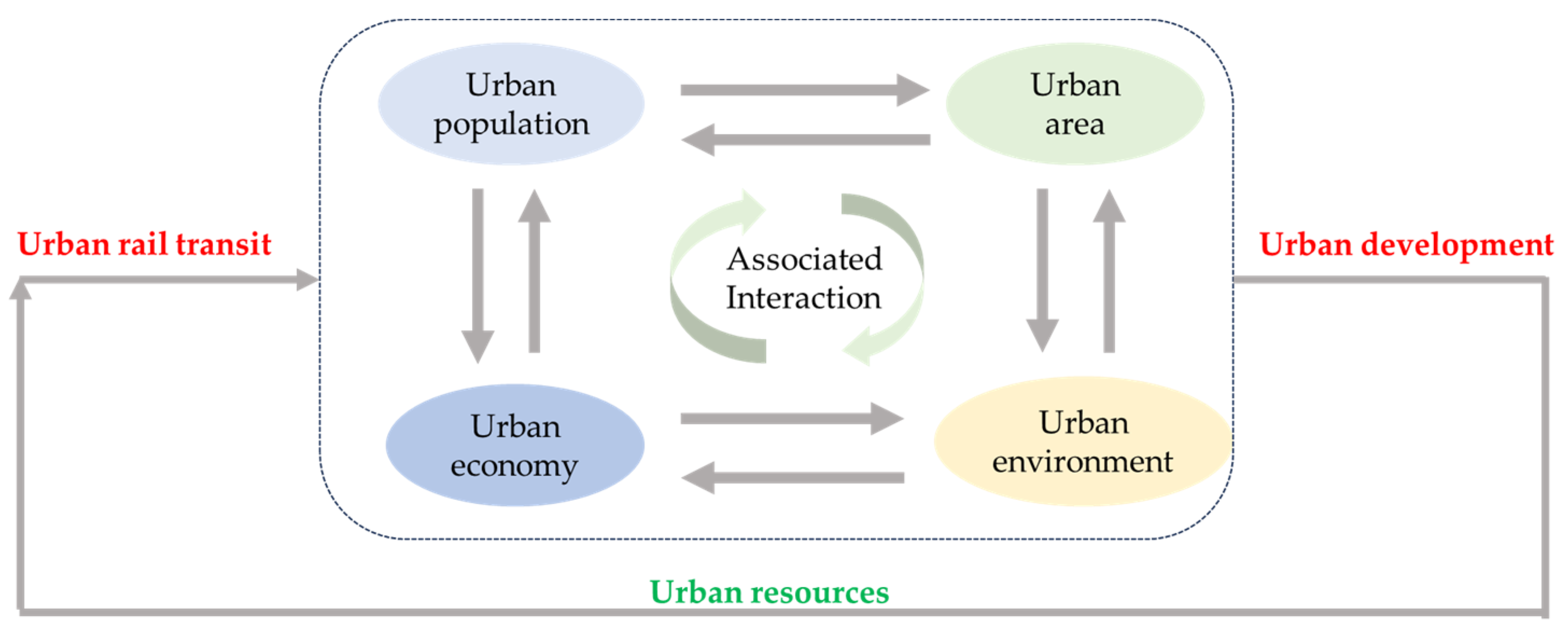
3.1. System Boundary

Considering various factors influencing UD, this study explored a reasonable URTN scale that matches UD. In this study, factors included the economic development level, population growth trends, land use, and environment. The environment is mainly represented by road traffic pollution. The road traffic encompasses the use of private cars, taxis, and buses for traveling. New shared mobility options [41], such as ride-sourcing, are included as the road traffic flow in the model. Other transportation modes, such as motorcycles and bike-sharing [42,43], are not considered. Therefore, the system boundary involves six subsystems: URT, UD, urban economy, urban population, urban land, and urban environment subsystems.

3.2. Causal Feedback Diagram

A causal feedback diagram can graphically present the causal relationships between factors in a system, with factors connected by arrows to represent a causal relationship. Figure 2 presents the causal feedback diagram of the URT and UD. The blue bold variables in the diagram illustrate the causal relationships among the six subsystems within the system boundary.

Table 1. Symbols of causality.

Symbol	Meaning
	A and B change in the same direction
	A and B change in the opposite direction
	Positive feedback loop
	Negative feedback loop

lists the meaning of the symbols in the figure. The main causal loops in the model are listed below:

R1: the scale of URTN $\stackrel{+}{\to }$ GDP $\stackrel{+}{\to }$ UD index $\stackrel{+}{\to }$ the scale of URTN

The increase in the URTN scale will stimulate the growth of the urban economy. When the economy grows, it will promote UD, and the city’s development will provide more financial resources for URT construction. This is a positive feedback loop.

R2: the scale of URTN $\stackrel{+}{\to }$ Population $\stackrel{+}{\to }$ UD index $\stackrel{+}{\to }$ the scale of URTN

The increase in the URTN scale will attract an in-migration population, and population growth will promote UD. With the city’s development, URT construction is supported. This is a positive feedback loop.

R3: the scale of URTN $\stackrel{+}{\to }$ Built-up area $\stackrel{+}{\to }$ UD index $\stackrel{+}{\to }$ the scale of URTN

The URT will promote the expansion of the built-up area. This will promote UD. As the city develops, the scale of URTN is benefitted. This is a positive feedback loop.

B1: the scale of URTN $\stackrel{—}{\to }$ Traffic congestion $\stackrel{—}{\to }$ Air pollutant concentrations $\stackrel{—}{\to }$ UD index $\stackrel{+}{\to }$ the scale of URTN

The URT will alleviate traffic congestion and reduce traffic emissions, thereby contributing to air quality levels and promoting UD. UD is beneficial for the scale of URTN. This is a negative feedback loop.

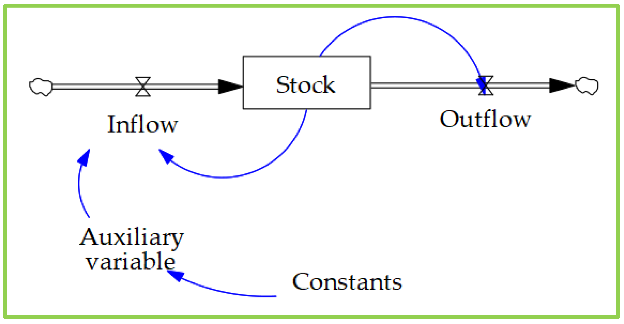
3.3. Stock–Flow Diagram

Building upon the causal feedback diagram, the stock–flow diagram was further established. The stock–flow diagram is the foundation for quantitatively depicting the relationship between the URT and UD. This diagram has four variables. ① The stocks, namely the level variable, represent resources of each factor that are accumulated, such as the accumulation of the URTN scale. ② The flows, including inflow and outflow, are namely the rate variable. They represent variables that vary with time, such as the annual increment of the URTN scale. ③ The auxiliary variables represent the intermediate variables that describe the system’s behavior. ④ The constants are numerical values. Figure 3 presents the meaning of symbols in the stock–flow diagram. The stock–flow diagram, presented in Figure 4, includes 10 stocks and 14 flows.

The equation for flows can be represented by a differential equation. The stock’s value at time t is the net difference between the inflow and outflow between time t₀ and t plus the stock’s initial value at time t₀. The related equations are shown as follows.

$$\frac{d(stock)}{dt}=inflow(t)-outflow(t),$$

(1)

$$L_{stock}(t)=L_{stock}(t_0)+{\displaystyle {\int }_{t_0}^t\left[inflow(t)-outflow(t)\right]} dt,$$

(2)

3.4. SD Equations

The system equations quantitatively describe the interaction between subsystems. First, we established the LV model to depict the mutualistic relationships. Next, its stability was analyzed before the model was integrated into the SD equations.

3.4.1. LV Mutualism Model

The LV model is based on the logistic model and examines the relationship among species. The logistic model is a vital mathematical tool for studying the evolutionary dynamics of biological populations within a finite space [44]. This process is often denoted by an S-shaped curve.

Assuming UD follows ecological principles of the logistic model [45,46], the “species” in the city are all consistent with the logistic growth function, such as the URTN scale, number of motor vehicles, and number of bus passengers [35,37,47]. In this study, the UD index was used to represent UD, and 11 indicators (

Table A1. Urban Development Indicators.

Number	Variable Name	Unit	Sample Size	Mean	Standard Error
1	Population	per ten thousand people	170	1471.13	704.81
2	Urbanization rate	%	170	0.0787	0.121
3	Built-up area	km2	170	799.76	351.69
4	GDP	hundred million	170	10,919.81	8022.71
5	General public budget revenue	hundred million	170	1549.24	1487.99
6	Infrastructure investment amount	hundred million	170	1598.36	1301.22
7	Road length	km	170	5054.62	1931.44
8	The number of cars	ten thousand vehicles	170	237.84	151.11
9	The total passenger volume of URT	ten thousand person-times	170	80,385	105,944.70
10	The total passenger volume of Bus	ten thousand person-times	170	200,503	130,822.70
11	Urban rail ownership rate	%	170	0.115	0.954

in Appendix A) from 10 cities were selected to calculate this index by using the entropy weighting method.

Table A2. Urban Development Index.

Year	Beijing	Tianjin	Shanghai	Guangzhou	Dalian	Wuhan	Chongqing	Shenzhen	Nanjing	Chengdu
2003	0.230	0.075	0.204	0.113	0.039	0.036	0.132	0.063	0.049	0.056
2004	0.261	0.085	0.233	0.124	0.043	0.048	0.139	0.079	0.057	0.063
2005	0.280	0.099	0.262	0.137	0.048	0.058	0.153	0.099	0.073	0.072
2006	0.293	0.114	0.282	0.168	0.055	0.064	0.170	0.117	0.079	0.080
2007	0.321	0.124	0.325	0.195	0.066	0.074	0.188	0.137	0.087	0.089
2008	0.391	0.141	0.359	0.213	0.08	0.093	0.205	0.150	0.095	0.102
2009	0.433	0.158	0.397	0.237	0.09	0.109	0.224	0.172	0.101	0.118
2010	0.488	0.172	0.453	0.299	0.111	0.125	0.256	0.199	0.133	0.137
2011	0.528	0.194	0.478	0.368	0.131	0.138	0.297	0.253	0.150	0.160
2012	0.573	0.226	0.489	0.393	0.137	0.163	0.336	0.279	0.167	0.190
2013	0.627	0.253	0.527	0.419	0.142	0.184	0.378	0.302	0.185	0.216
2014	0.663	0.272	0.559	0.441	0.143	0.209	0.414	0.326	0.223	0.249
2015	0.672	0.288	0.603	0.380	0.170	0.243	0.451	0.347	0.252	0.274

(Appendix A) presents the results of the calculation.

The logistic function is presented in Equation (3).

$$\frac{dx(t)}{dt}=r_{t}x(t)(1-\frac{x(t)}{K}),$$

(3)

where $x(t)$ is the UD index or URTN scale in year t, K is the carrying capacity of UD or URTN scale, and $(1-\frac{x(t)}{K})$ is the coefficient of Logistic, which means the resources available for UD or URTN scale growth. $r_t$ is the natural growth rate [48], and the function is shown in Equation (4).

$$r_t=\frac{K}{K-x(t)}\times \frac{dx(t)}{dt},$$

(4)

The LV mutualism model is an extension of the logistic function. The mutualism coefficients ($\alpha ,\beta$), which represent the interaction relationship, were added to the logistic growth function. The function is shown in Equation (5).

$$\left\{\begin{array}{l}\frac{d{x}_1(t)}{dt}=r_1(t)x_1(t)(1-\frac{x_1(t)}{K_1}+\frac{\alpha x_2(t)}{K_2})\\ \frac{d{x}_2(t)}{dt}=r_2(t)x_2(t)(1-\frac{x_2(t)}{K_2}+\frac{\beta x_1(t)}{K_1})\end{array}\right.,$$

(5)

where $x_1(t)$ and $x_2(t)$ represent the URTN scale and the scale of the UD index; $r_1(t)$ $r_2(t)$ represent their growth rates, respectively; $K_1$ and $K_2$ denote their maximum growth scales, respectively; $\alpha$ denotes the effect of UD on the URTN scale. $\alpha <0$ means that the city is no longer willing to provide resources for URT construction. $\alpha >0$ indicates that UD has a promoting effect on the URT. $\beta$ denotes the effect of the URT on UD. $\beta <0$ indicates that URT has not played a role in promoting UD, whereas $\beta >0$ means that URT has a promoting effect on UD.

The concept of mutualism coefficients originates from ecology. In an ecosystem, there are mutualistic relationships between species and the ecological environment (EE). The EE provides resources that promote the growth of the species. The species, in turn, produces resources that foster the EE. The concept of mutualism coefficients was proposed by Ecologists MacArthur and Levins [49,50]. For example, the promotion of EE to the species is represented by the proportion of resources to species provided by the EE relative to the total EE resources. Conversely, the contribution of the species to the EE is represented by the proportion of resources generated by the species relative to the total EE resources.

In urban systems, a similar mutualistic relationship exists between the URT and UD. For instance, UD provides more resources to the URT, such as investment and land, which promotes the expansion of the URT. The URT, in turn, promotes UD by increasing economic activities. Based on this, the mutualism coefficients ($\alpha ,\beta$) were established. The essence of $\alpha$ is the proportion of urban resources used by the URT, such as financial, passenger flow, and land resources. The essence of $\beta$ is the contribution rate of the URT to UD, which includes the annual increment of GDP, decreased increment of air pollutants, alleviation of traffic congestion, and urban land expansion. The related equations are shown as follows.

$${\alpha }_i={\displaystyle \sum _{k=1}^n\frac{C_{ik}}{R_{ik}}},$$

(6)

$${\beta }_i={\displaystyle \sum _{h=1}^n\frac{Q_{ih}}{P_{ih}}},$$

(7)

where ${\alpha }_i$ is the rate of urban resources consumed by the URT in year i; $C_{ik}$ represents the resource k consumed by the URT in year i, and $R_{ik}$ is the total resource of k in year i. ${\beta }_i$ is the contribution rate of the URT to UD in year i; $Q_{ih}$ represents the contribution of URT to resource h in year i, and $P_{ih}$ is the total resource of h in year i.

3.4.2. Stability Analysis of the LV Model

The evolution trends of the URT and UD can be studied by conducting the stability analysis of the model. Set,

$$\left\{\begin{array}{l}f(x_1,x_2)=r_1{x}_1(1-\frac{x_1}{K_1}+\frac{\alpha x_2}{K_2})=0\\ g(x_1,x_2)=r_2{x}_2(1-\frac{x_2}{K_2}+\frac{\beta x_1}{K_1})=0\end{array}\right.,$$

(8)

Four equilibrium points were calculated, which are $P_1(0,0)$, $P_2(K_1,0)$, $P_3(0,K_2)$, $P_4(\frac{(1+\alpha )K_1}{1-\alpha \beta },\frac{(1+\beta )K_2}{1-\alpha \beta })$. The Taylor expansion of Equation (6) takes the primary term to construct the Jacobi matrix denoted as D.

Table 2. Equilibrium points and equilibrium conditions.

Equilibrium Point	p	q	Stability Condition
$P_1(0,0)$	$-(r_1+r_2)$	$r_1{r}_2$	Unstable
$P_2(K_1,0)$	$r_1-r_2(1+\beta )$	$-r_1{r}_2(1+\beta )$	Unstable
$P_3(0,K_2)$	$r_2-r_1(1+\alpha )$	$-r_1{r}_2(1+\alpha )$	Unstable
$P_4(\frac{(1+\alpha )K_1}{1-\alpha \beta },\frac{(1+\beta )K_2}{1-\alpha \beta })$	$\frac{r_1(1+\alpha )+r_2(1+\beta )}{1-\alpha \beta }$	$\frac{r_1{r}_2(1+\alpha )(1+\beta )}{1-\alpha \beta }$	$\alpha \beta <1$

presents the equilibrium stability analysis of the four equilibrium points for the mutualism model. The mutualistic relationships between the URT and UD are investigated, which is only relevant when the equilibrium point is in the first quadrant of the coordinate system. Therefore, when $\alpha \beta <1$, the development status of URT and UD is stable for the equilibrium point $P_4$.

$$D=\left(\begin{array}{cc}\frac{\partial f}{\partial x_1}& \frac{\partial f}{\partial x_2}\\ \frac{\partial g}{\partial x_1}& \frac{\partial g}{\partial x_2}\end{array}\right)=\left(\begin{array}{cc}{r}_1(1-\frac{2x_1}{K_1}+\frac{\alpha x_2}{K_2})& r_1{x}_1\frac{\alpha }{K_2}\\ r_2{x}_2\frac{\beta }{K_1}& r_2(1-\frac{2x_2}{K_2}+\frac{\beta x_1}{K_1})\end{array}\right),$$

(9)

$$p=-(\frac{\partial f}{\partial x_1}+\frac{\partial g}{\partial x_2}){|}_{P_i},i=1,2,3,4$$

(10)

$$q=\det D{|}_{P_i},i=1,2,3,4$$

(11)

The stability analysis unveiled that mutualism coefficients determine the trends of the URT and UD. Simulating the scenarios produced by different coefficients can provide decision support for policymakers. Different scenarios will be specifically addressed in the Discussion section.

3.4.3. SD Equations

The SD equations were established in the stock–flow diagram, which comprises six subsystems. The equations are built in two parts: one part is the mutualistic relationships equations, and the other part is the four subsystem equations, apart from the URT and UD subsystems. For clarity, the equations were expressed with a uniform notation.

Table 3. The notation and meaning of SD equations.

Notation	Meaning	Example
L	the stocks	$L_{urts}(t)$ denotes the network length of URT.
R	the flows	$R_{urts}(t)$ is the annual increment of the network length.
A	the rate of change	$A_{urts}(t)$ denotes the growth rate of the network length.

presents the notions and meanings.

① Mutualistic relationships equations

The network length of the URT represents the URTN scale. The length of the URT and the UD index are set as the system stock, and the annual increment is set as the system flow. Equations (3) and (5) are introduced into the SD model. UD is influenced by the urban economy, population, land use, and environmental subsystems. The equations are presented as follows.

$$L_{urts}(t)=L_{urts0}+{\displaystyle {\int }_0^t{R}_{urts}(t})dt,$$

(12)

$$R_{urts}(t)=\frac{d{L}_{urts}(t)}{dt}=L_{urts}(t)\times A_{urts}(t)\times (1-\frac{L_{urts}(t)}{Ma{x}_{urts}}+\frac{\alpha \times L_{cd}(t)}{Ma{x}_{cd}}),$$

(13)

$$\alpha =delay((\frac{L_{urts(t)}\times C_{urts}}{L_{gdp}(t)}\times 0.5+R_{urt\_share}\times 0.5),8),$$

(14)

$$L_{cd}(t)=L_{cd0}+{\displaystyle {\int }_0^t{R}_{cd}(t})dt,$$

(15)

$$R_{cd}(t)=\frac{d{L}_{cd}(t)}{dt}=L_{cd}(t)\times A_{cd}(t)\times (1-\frac{L_{cd}(t)}{Ma{x}_{cd}}+\frac{\beta \times L_{urts}(t)}{Ma{x}_{urts}}),$$

(16)

$$\beta =\frac{R_{gdp}(t)}{L_{gdp}(t)}\times {\omega }_1+\frac{C_{traffic\_congestion}(t)-1}{C_{traffic\_congestion}(t)}\times {\omega }_2+\frac{R_{in\_pollution}(t)}{L_{air\_pollution}(t)}\times {\omega }_3+\frac{R_{move}(t)}{L_{pop}(t)}\times {\omega }_4+\frac{R_{land}(t)}{L_{land}(t)}\times {\omega }_5$$

(17)

where $L_{urts0}$ represents the initial value of the network length; $L_{cd0}$ represents the initial value of the UD index; $L_{cd}(t)$ is the UD index in year t; $L_{gdp}(t)$ is the GDP in year t; $L_{pop}(t)$ is the population size in year t; $L_{land}(t)$ is the built-up area in year t; $L_{air\_pollution}(t)$ represents air pollutants in year t; $R_{urt\_share}$ is the sharing ratio of URT; 0.5 is the weighting factor; $R_{cd}(t)$ is the annual increment of the UD index; $R_{gdp}(t)$ is the annual increment of GDP; $R_{in\_pollution}(t)$ in annual increment of air pollutants in year t; $R_{move}(t)$ is the migration population increment in year t; $R_{land}(t)$ is the annual increment of the built-up area; ${\omega }_i(i=1,2,\dots ,5)$ represent the weight value for different factors; $A_{cd}(t)$ is the growth rate of the UD index; $Ma{x}_{urts}$ is the maximum scale of URTN; $Ma{x}_{cd}$ is the maximum scale of UD index; $C_{urts}$ is the cost of URT; $C_{traffic\_congestion}(t)$ is road traffic congestion in year t; $\alpha$ is the mutualism coefficient of UD on the URT; $\beta$ is the mutualism coefficient of the URT on UD.

② Other equations

There are four subsystem equations. The urban economy is represented by GDP. Urban land use is indicated by the built-up area, and the urban environmental level is denoted by air pollutants. The GDP, population, built-up area, and air pollutants are established as the system stocks, and their annual increments are established as system flows. The equations are given as follows.

$$L_{gdp}(t)=L_{gdp0}+{\displaystyle {\int }_0^t{R}_{gdp}(t})dt,$$

(18)

$$R_{gdp}(t)=\frac{d{L}_{gdp}(t)}{dt}=L_{gdp}(t)\times A_{gdp}(t)\times (1-\frac{L_{gdp}(t)}{Ma{x}_{gdp}})+delay((L_{urts}(t)\times {\gamma }_1),8),$$

(19)

$$L_{pop}(t)=L_{pop0}+{\displaystyle {\int }_0^t(R_{pop}(t})+R_{move}(t))dt,$$

(20)

$$R_{pop}(t)=\frac{d{L}_{pop}(t)}{dt}=L_{pop}(t)\times A_{pop}(t)\times (1-\frac{L_{pop}(t)}{Ma{x}_{pop}}),$$

(21)

$$R_{move}(t)=L_{urts}(t)\times \rho ,$$

(22)

$$L_{land}(t)=L_{land0}+{\displaystyle {\int }_0^t{R}_{land}(t})dt,$$

(23)

$$R_{land}(t)=\frac{d{L}_{land}(t)}{dt}=L_{land}(t)\times A_{land}(t),$$

(24)

$$A_{land}(t)=L_{urts}(t)\times {\gamma }_2+L_{roads}(t)\times {\gamma }_3,$$

(25)

$$L_{air\_pollution}(t)=L_{air\_pollution0}+{\displaystyle {\int }_0^t(R_{in\_pollution}(t})-R_{out\_pollution}(t))dt,$$

(26)

$$R_{in\_pollution}(t)=(P_{car}(t)+P_{texi}(t)+P_{bus}(t))\times {\gamma }_{emission}\times V_{ave\_speed},$$

(27)

$$V_{ave\_speed}={\gamma }_{ave\_speed}\times C_{traffic\_congestion}(t),$$

(28)

$$R_{out\_pollution}(t)=L_{air\_pollution}(t)\times A_{out\_pollution}(t),$$

(29)

where L_gdp0 is the initial GDP value; $L_{pop0}$ is the initial population size value; $L_{land0}$ is the initial built-up area value; $L_{air\_pollution0}$ is the initial value of air pollutants; $L_{road}(t)$ represents road lengths in year t; $R_{pop}(t)$ is the annual increment of population; $R_{out\_pollution}(t)$ is the dissipation of air pollutants in year t; $A_{gdp}(t)$ is the GDP growth rate; $A_{pop}(t)$ is the growth rate of the population size; $A_{land}(t)$ is the growth rate of the built-up area; $A_{out\_pollution}(t)$ is the dissipation rate; $Ma{x}_{gdp}$ is the maximum scale of GDP; $Ma{x}_{pop}$ is the maximum scale of population; ${\gamma }_1$ is the elasticity coefficient of the URT on urban economy; $\rho$ is the migration coefficient; ${\gamma }_2$ is the contribution coefficient of the URT to the built-up area; ${\gamma }_3$ is the contribution coefficient of the road to the built-up area; $V_{ave\_speed}$ is average travel speed; ${\gamma }_{emission}$ is the coefficient of emissions. $P_{car}(t)$, $P_{texi}(t)$, and $P_{bus}(t)$ represent the road travel volumes of cars, taxis, and buses; ${\gamma }_{ave\_speed}$ is the coefficient between traffic congestion and the average speed.

4. Case Study

The Beijing URT in China is employed as a case study here. The Vensim PLE (10.0.0) software platform was utilized for simulation.

4.1. Data Input

The data were collected from the Beijing Statistical Yearbook [51], Beijing Transport Development Annual Report [52], China Urban Construction Statistical Yearbook [53], and China Urban Statistical Yearbook [54]. The starting year of the model was 1984, with the total simulation period set to 60 years and a time step of 1 year. The initial value of the 10 stocks in 1984 was input into the model. The parameter K in Equation (3) of the URTN scale was estimated based on historical statistics using SPSS, as shown in

Table A3. The Logistic function for parameter estimation of the Beijing URT scale.

Parameter	Estimated Value	Standard Error	p-Value	R2	Confidence Level
K	3028.622	34.385	0.001	0.994	95%
a	2488.890	568.656	0.000
b	0.124	0.005	0.000

(Appendix A).

Table 4. Initial value of key parameters in the model.

Variable Name	Initial Value	Unit
Scale of URTN	41	km
Maximum scale of URTN	3028.66	km
UD index	0.1	dimensionless
Maximum UD index	1	dimensionless
GDP	216	hundred million
Road length	1436	km
Population	965	ten thousand
Built-up area	366	km2
Air pollutants	100	thousand tons
Number of private cars	8.7	ten thousand
Number of taxies	0.4279	ten thousand
Number of buses	0.4066	ten thousand

presents the initial values of the stocks of the model.

4.2. Model Validation

Currently, two methods are available for testing the SD-LV model. One is to set different simulation time steps and observe whether the SD model produces stable output or not [35]. The other method involves selecting the simulation results of certain variables and comparing them with actual statistics. If the errors are all <10%, then the model is considered effective [55,56].

First, the different simulation time steps are set to observe the outputs. For example, the simulation results for the URTN scale are presented in Figure 5. Curves 1, 2, and 3 represent different simulation results when the time step was set to year, quarter, and month, respectively. The results indicate that the system’s behavior is stable, and the SD-LV model is robust.

Second, the simulation value of the URTN scale, GDP, and population is selected and compared with the actual statistics.

Table 5. Results of error analysis.

Variable/Year		2017	2018	2019	2020	2021
Scale of URTN	Actual value	587.8	636	699	727	783
	Simulation Value	580.24	623.51	672	730.7	793.3
	Error	−1.28%	−1.96%	−4.3%	0.51%	1.32%
GDP	Actual value	31,387	30,319.97	35,371	36,103	40,269.6
	Simulation Value	29,780.2	32,573.8	35,500.4	38,804.7	42,554.1
	Error	−8.01	0.78%	−8.19%	7.48%	5.67%
Population	Actual value	2170.8	2154.2	2153	2189	2188.6
	Simulation Value	1980.01	2001	2023	2024.11	2042.89
	Error	−8.79%	−7.11%	−6.04%	−7.53%	−6.66%

presents the specific results. The errors fall within acceptable limits. This indicates that the SD-LV model is effective and can be used in further studies.

4.3. Results and Discussion

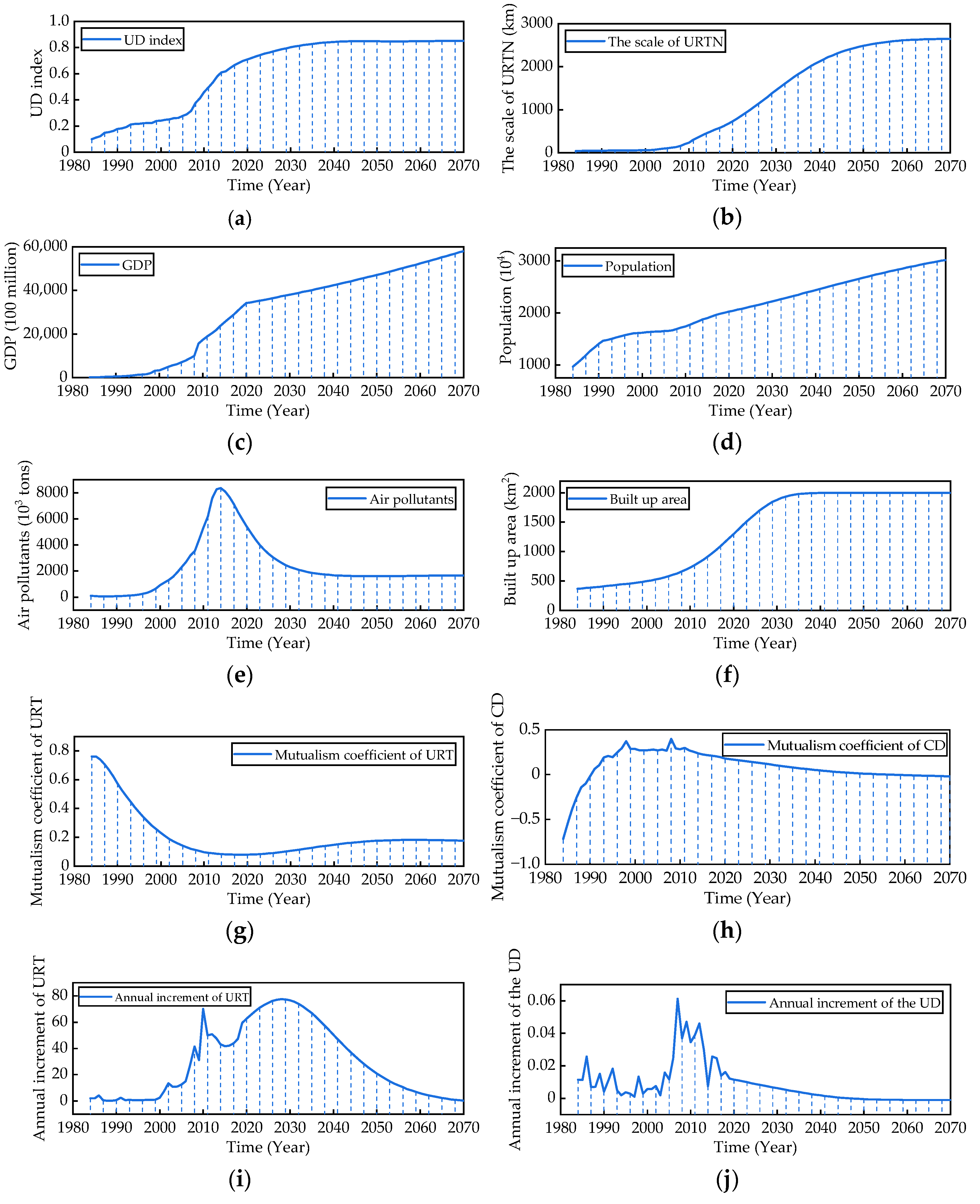
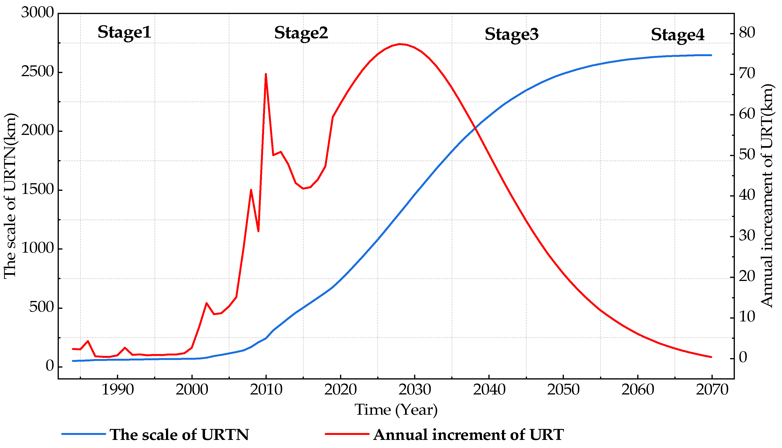
4.3.1. The Simulation Results

Figure 6 presents the simulation results. The UD index (a) and the URT scale (b) present the characteristics of the “S” growth curve. GDP (c), population (d), and built-up area (f) are increasing gradually. The environment (e) has an “inverted U” curve. $\alpha$, which is the mutualism coefficient of URT (g), is between 0 and 1; $\beta$, which is the mutualism coefficient of UD (h), is between −1 and 1. According to the stability analysis of the LV model (Section 3.4.2), $\alpha \beta <1$, the system behavior is stable. The model predicts that the URTN scale will reach 1786 km by 2035, and the UD index of Beijing will reach 0.8.

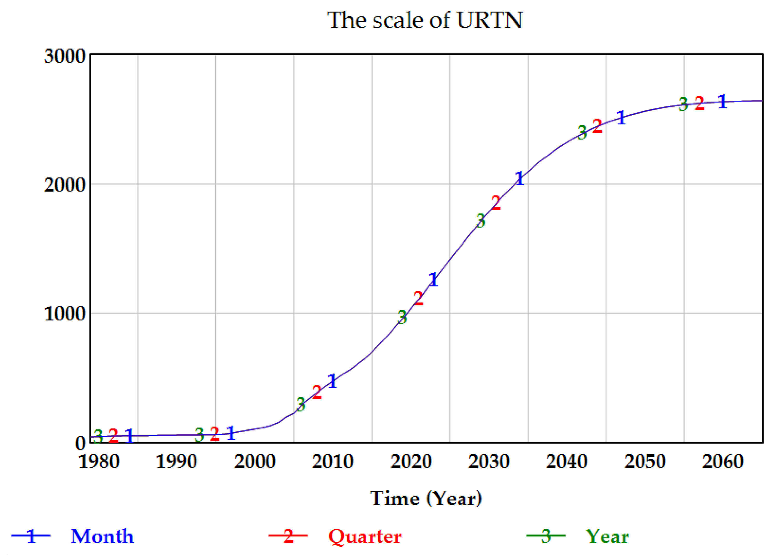
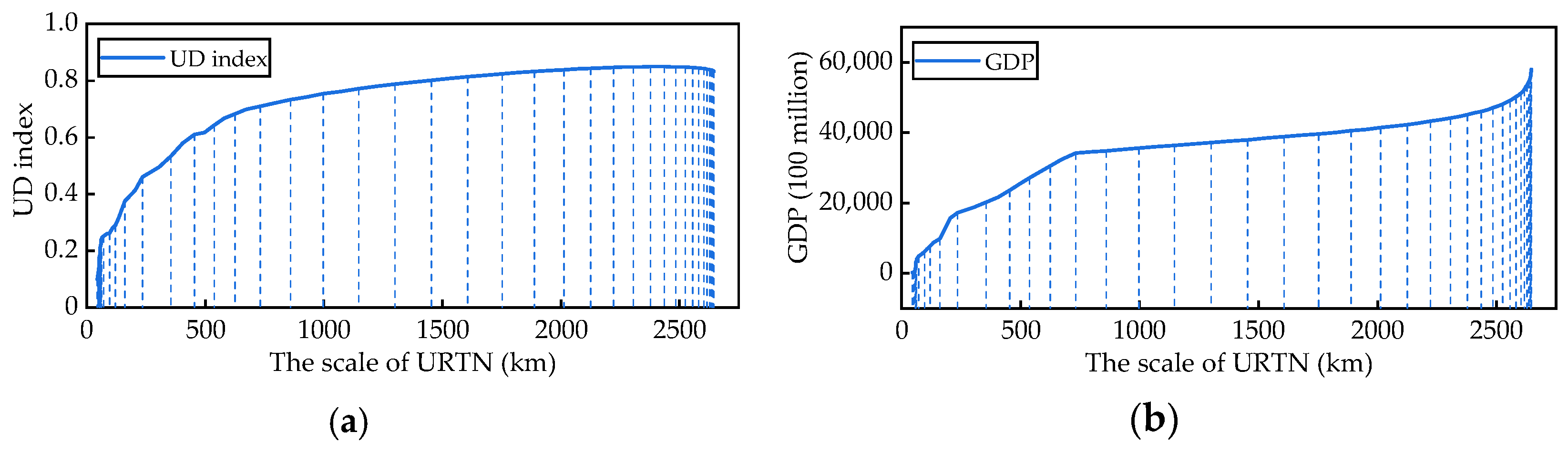
4.3.2. The Scale of URTN

Figure 7 shows the scale of the URTN (blue line) and the annual increment of the URT (red line). Figure 8 illustrates the relationship between the URTN scale and other factors. The results are discussed in terms of four development stages (Stage 1: the initial growth stage; Stage 2: accelerated phase; Stage 3: decelerated phase; Stage 4: stabilization phase).

Stage 1: As seen in Figure 7, the scale was growing very slowly before 2000. This slow growth is attributable to the lower economic levels of Beijing during this period, with GDP being 43.8 billion yuan in 1990 and 233.2 billion yuan in 2000. This made it difficult to allocate substantial financial resources for URT development (Figure 8b). Additionally, high construction costs and lower URT construction levels lead to slow development. The UD index, GDP, population, and built-up area are growing with the URTN scale. However, air pollutants gradually increase (Figure 8d), consistent with the study by [21], which indicates that the impact of air pollution is not very significant in the initial stages of URT construction.

Stage 2: From 2000 to 2030, the Beijing URT construction entered an accelerated phase, especially before 2008, likely because of the significant increase in infrastructure investment for the 2008 Olympic Games. Additionally, the economy grew tremendously (Figure 8b), with GDP turning 1.3904 trillion yuan in 2010 and 3.6103 trillion yuan in 2020. A positive correlation exists between the URTN scale and urban economic growth, which is consistent with the results of [9]. The population surged to 21.89 million in 2020. Advances in science and technology lowered barriers to URT construction, which resulted in rapid construction. By the end of 2023, the scale had reached 836 km. As the scale increases, the urban land area also expands (Figure 8e), which further confirms the conclusions of [15]. The air pollutants decrease. This is consistent with the study of [21]; as the network scale expands, its effect on air quality becomes more critical.

Stage 3: As the network scale expands, most major urban areas will be well-served, which will reduce the necessity for rapid construction. From 2030 to 2050, the URT construction will enter a decelerated phase, with simulation results of the scale reaching 1786 km in 2035. As seen in Figure 8, the urban economy, population, and built-up area will remain at a high level of saturation.

Stage 4: After 2050, the URTN scale will enter a steady state and gradually approach saturation. The predicted scale can reach 2647.38 km.

4.3.3. Mutualism Coefficients

Figure 9 presents the mutualism coefficients of the URTN scale and UD index in Beijing. The blue line represents the mutualism coefficient of URT ($\alpha$), and the red line denotes the mutualism coefficient of UD ($\beta$). According to Section 3.4.2, $\alpha \beta <1$ means the dynamic interaction between the URT and UD is stable.

Before 1995, $0<\alpha <1,\beta <0$ shows that the city provided more resources to support the URT development within its limited resources, while the URT was unable to promote the city significantly because of its early development stage.

After 1995, $0<\alpha <1,\beta >0$ shows that the URT began to contribute to UD. However, as the city developed, the proportion of resources allocated to URT construction gradually decreased. This is because more resources were accumulated within the city over time. Additionally, advancements in technology have reduced the consumption of resources in URT construction.

Without changing the existing policies, the URT and UD in Beijing are in mutualistic relationships, and city policymakers can appropriately increase the resources invested in the URT so that it can contribute more to UD.

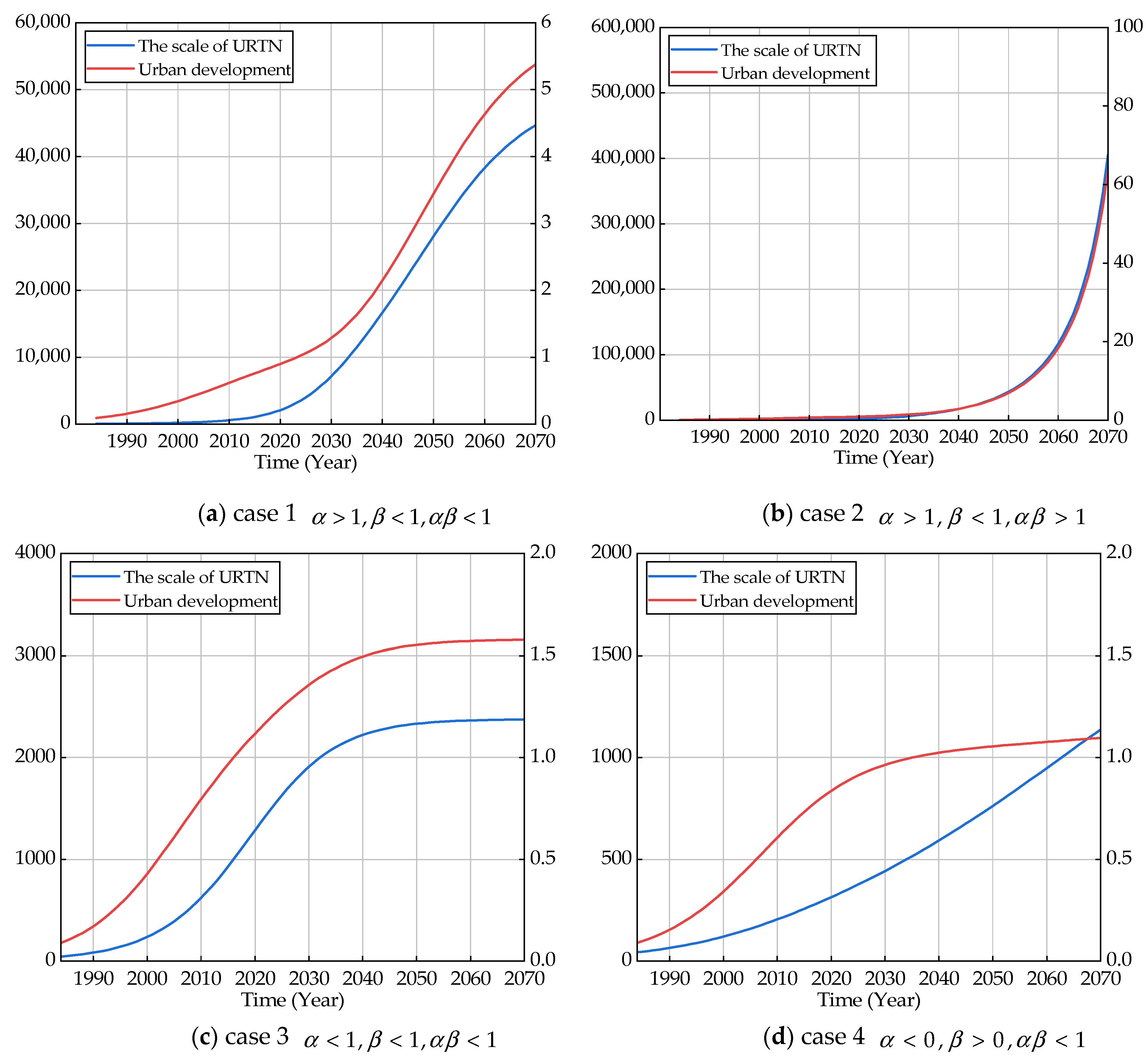
4.3.4. Different Scenarios of Mutualism Coefficient

The study calculated the reasonable scale by using mutualistic relationships. Different mutualistic relationships produce different results between the URT and UD. In this section, eight different mutualism coefficient scenarios are simulated (Figure 10), which provides decision support for policymakers and planners.

Case 1 ($\alpha >1,\beta <1,\alpha \beta <1$) indicates that the city has invested excessive resources in URT construction, resulting in an excessive scale. Although the URT promotes UD, the city is still burdened by resource consumption. This may occur in large cities with more financial resources.

Case 2 ($\alpha >1,\beta <1,\alpha \beta >1$) indicates that the relationship between the URT and UD is unstable. City policymakers need to adjust their investment policies promptly to address this instability.

Case 3 ($\alpha <1,\beta <1,\alpha \beta <1$) shows that the URT and UD are in mutualistic relationships, and both are in a good state of development.

Case 4 ($\alpha <0,\beta >0,\alpha \beta <1$) indicates that the city does not prioritize URT construction and has even halted its development.

Case 5 ($\alpha >0,\beta <0,\alpha \beta <1$) shows that excessive resources are invested in the URT, leading to its excessive consumption of UD resources and inhibition of UD. The URT and UD are in a poor development state. Urban policymakers should promptly adjust the urban investment policies and choose appropriate URT categories. This can happen in small- and medium-sized cities with more financial constraints.

Case 6 ($\alpha <0,\beta <0,\alpha \beta <1$) shows that the URT and UD are in a state of competition, resulting in neither of them obtaining more resources. Urban policymakers should pay close attention to the development trend and adjust policies so that they can gradually shift to mutualistic relationships.

Case 7 ($\alpha <-1,\beta <0,\alpha \beta <1$) indicates that the focus of UD has shifted to other aspects, and so the URT is considered a disadvantage and is gradually being replaced. This may be because urban policymakers have begun to doubt URT systems and have even considered removing them, which is similar to the removal of tram systems in many European cities in the last century.

Case 8 ($\alpha <0,\beta <-1,\alpha \beta <1$) indicates that urban resources are limited, and the URT competes with UD. Urban policymakers need to judge the timing and suitability of URT in the context of limited resources.

In summary, the URTN scale is crucial in network planning. Compared with traditional models using static indicators and qualitative analyses, the SD-LV model can assess the trends of the URT and UD based on mutualism coefficients. The findings provide valuable insights into URT planning decisions. Additionally, the model can simulate different scenarios, such as different investment policies, to foresee the future URTN scale. The methodology can be used by other cities to offer dynamic insight into urban planning policies.

5. Conclusions

In conclusion, a quantitative theoretical framework, the SD-LV model, was proposed to determine the reasonable scale of the URTN. In this framework, the SD model was used to simulate the dynamic interaction between the URT and UD. The LV model is introduced to calculate the scale, and mutualism coefficients are proposed to characterize the mutualistic relationships between the URT and UD. To the best of our knowledge, this is the first time that the SD model has been combined with the LV model of mutualism and applied to address this issue. The model proposed was verified by using the dataset from the Beijing URT and UD. The study offers quantitative theoretical insights for determining the reasonable scale. The main conclusions are listed as follows:

(1) The SD model can simulate the dynamic interaction between the URT and UD. Through model deduction, URT was found to contribute to UD by promoting the urban economy, aggregating population size, expanding urban land, and improving the urban environmental level;

(2) The dynamics mutualistic relationships exist between the URT and UD, which is consistent with the LV mutualism model. The development trends of the URT and UD are determined by the mutualism coefficients;

(3) The URTN scale is directly related to the mutualism coefficients, denoted as $\alpha$ and $\beta$. $0<\alpha <1,0<\beta <1,$ indicates that the URTN scale is reasonable. When $\alpha >1$, the city has invested excessive resources in URT construction, resulting in an excessive scale; $\alpha <0$ shows that the city does not prioritize URT construction and has even halted its development. $\beta <0$ demonstrates that the URT has not played a role in promoting UD, possibly because of inadequate construction or being in the early developmental stages. The results provide decision support for planners and policymakers;

(4) The model was validated by using a dataset of the Beijing URTN from 2017 to 2021. The simulation errors of the URTN scale ranged from −4.3% to 1.32%, demonstrating the robustness and effectiveness of the model.

However, this study has several limitations. For example, in the mutualism coefficients of the URT to the resource occupancy capacity, only urban economy and land use have been counted. Future studies should expand the scope to include additional factors, such as the labor force, policy support, and technological level. New transportation modes have recently emerged, such as bike-sharing. These factors should be included to optimize the model in future studies.

References

1. Huang, C.; Xia, Y. Study on the Effect of Urban Rail Transit on Regional Economy. Adv. Mater. Res. 2012, 361, 1684–1688. [Google Scholar] [CrossRef]
2. Calvo, F.; de Oña, J.; Arán, F. Impact of the Madrid subway on population settlement and land use. Land. Use. Policy 2013, 31, 627–639. [Google Scholar] [CrossRef]
3. Sekar, S.P.; Gangopadhyay, D. Impact of rail transit on land use and development: Case study of suburban rail in Chennai. J. Urban. Plan. Dev. 2007, 143, 04016038. [Google Scholar] [CrossRef]
4. Jiao, L.; Luo, F.; Wu, F.; Zhang, Y.; Huo, X.; Wu, Y. Exploring the Interactive Coercing Relationship between Urban Rail Transit and the Ecological Environment. Land 2022, 11, 836. [Google Scholar] [CrossRef]
5. Shepherd, S.P. A review of system dynamics models applied in transportation. Transp. Metrica B Transp. Dyn. 2014, 2, 83–105. [Google Scholar] [CrossRef]
6. Kunc, M.; Mortenson, M.J.; Vidgen, R. A computational literature review of the field of System Dynamics from 1974 to 2017. J. Simul. 2018, 12, 115–127. [Google Scholar] [CrossRef]
7. Wangersky, P.J. Lotka-Volterra population models. Ann. Rev. Ecol. Syst. 1978, 9, 189–218. [Google Scholar] [CrossRef]
8. Zhang, Z. Mutualism or cooperation among competitors promotes coexistence and competitive ability. Ecol. Model. 2003, 164, 271–282. [Google Scholar] [CrossRef]
9. Li, H.; Wang, Z.; Guo, X. Urban rail transit and economic growth—An empirical analysis based on China’s cities panel data. In Proceedings of the 5th International Conference on Industrial Economics System and Industrial Security Engineering (IEIS), Toronto, ON, Canada, 3–6 August 2018; IEEE: Toronto, ON, Canada, 2018; pp. 1–5. [Google Scholar] [CrossRef]
10. Lee, E.H.; Shin, H.; Cho, S.H.; Kho, S.-Y.; Kim, D.K. Evaluating the Efficiency of Transit-Oriented Development Using Network Slacks-Based Data Envelopment Analysis. Energies 2019, 12, 3609. [Google Scholar] [CrossRef]
11. Wang, Z.; Li, X.; Bobylev, N.; Li, S.; Liu, J. Coupling Coordination of “Urban Rail Transit—Social Economy” Composite System. Infrastructures 2022, 7, 56. [Google Scholar] [CrossRef]
12. Liu, D. Analytical forecasting of population distribution over years in a new rail transportation corridor. J. Urban. Plan. Dev. 2016, 142, 04016021. [Google Scholar] [CrossRef]
13. Lee, E.H.; Lee, H.; Kho, S.Y.; Kim, D.K. Evaluation of transfer efficiency between bus and subway based on data envelopment analysis using smart card data. KSCE J. Civ. Eng. 2019, 23, 788–799. [Google Scholar] [CrossRef]
14. Li, Y. Coordination between Urban Rail Transit Development and Urban Population Change. In Proceedings of the CICTP, Xi’an, China, 14–16 August 2020; pp. 2942–2953. [Google Scholar] [CrossRef]
15. Ratner, K.A.; Goetz, A.R. The reshaping of land use and urban form in Denver through transit-oriented development. Cities 2013, 30, 31–46. [Google Scholar] [CrossRef]
16. Bhattacharjee, S.; Goetz, A.R. The rail transit system and land use change in the Denver metro region. J. Transp. Geogr. 2016, 54, 440–450. [Google Scholar] [CrossRef]
17. Liu, W.; Wang, J. Evaluation of coupling coordination degree between urban rail transit and land use. Int. J. Commun. Syst. 2021, 34, e4015. [Google Scholar] [CrossRef]
18. Song, J.; Abuduwayiti, A.; Gou, Z. The role of subway network in urban spatial structure optimization-Wuhan city as an example. Tunn. Undergr. Sp. Tech. 2023, 131, 104842. [Google Scholar]
19. Guo, S.; Chen, L. Can urban rail transit systems alleviate air pollution? Empirical evidence from Beijing. Growth Chang. 2019, 50, 130–144. [Google Scholar] [CrossRef]
20. Ou, Y.; Zheng, J.; Nam, K.M. Impacts of Urban Rail Transit on On-Road Carbon Emissions: A Structural Equation Modeling Approach. Atmosphere 2022, 13, 1783. [Google Scholar] [CrossRef]
21. Ou, Y.; Song, W.; Nam, K.M. Metro-line expansions and local air quality in Shenzhen: Focusing on network effects. Transp. Res. Part D Transp. Environ. 2024, 126, 103991. [Google Scholar] [CrossRef]
22. Gendron-Carrier, N.; Gonzalez-Navarro, M.; Polloni, S.; Turner, M.A. Subways and urban air pollution. Am. Econ. J-Appl. Econ. 2022, 14, 164–196. [Google Scholar] [CrossRef]
23. Tan, Y.; Jiao, L.; Shuai, C.; Shen, L. A system dynamics model for simulating urban sustainability performance: A China case study. J. Clean. Prod. 2018, 199, 1107–1115. [Google Scholar] [CrossRef]
24. Xing, L.; Xue, M.; Hu, M. Dynamic simulation and assessment of the coupling coordination degree of the economy-resource-environment system: Case of Wuhan City in China. J. Environ. Manag. 2019, 230, 474–487. [Google Scholar] [CrossRef]
25. Xu, J.; Kang, J. Comparison of ecological risk among different urban patterns based on system dynamics modeling of urban development. J. Urban. Plan. Dev. 2017, 143, 04016034. [Google Scholar] [CrossRef]
26. Bach, P.; Tustanovski, E.; Andrew, W.H.; Yung, K.L.; Roblek, V. System dynamics models for the simulation of sustainable urban development: A review and analysis and the stakeholder perspective. Kybernetes 2020, 49, 460–504. [Google Scholar] [CrossRef]
27. Su, Y.; Liu, X.; Li, X. Research on traffic congestion based on system dynamics: The case of Chongqing, China. Complexity 2020, 2020, 6123896. [Google Scholar] [CrossRef]
28. Yang, H.; Wang, W.; Wei, B. System dynamics for urban traffic jam management in beijing. Environ. Eng. Manag. J. 2015, 14, 1875–1886. [Google Scholar] [CrossRef]
29. Yang, Y.; Zhang, P.; Ni, S. Assessment of the impacts of urban rail transit on metropolitan regions using system dynamics model. Transp. Res. Procedia 2014, 4, 521–534. [Google Scholar] [CrossRef]
30. Chen, Y.; Stasinopoulos, P.; Shiwakoti, N.; Khan, S.K. Using System Dynamics Approach to Explore the Mode Shift between Automated Vehicles, Conventional Vehicles, and Public Transport in Melbourne, Australia. Sensors 2023, 23, 7388. [Google Scholar] [CrossRef]
31. Mylonakou, M.; Chassiakos, A.; Karatzas, S.; Liappi, G. System Dynamics Analysis of the Relationship between Urban Transportation and Overall Citizen Satisfaction: A Case Study of Patras City, Greece. Systems 2023, 11, 112. [Google Scholar] [CrossRef]
32. Bartuska, L.; Stopka, O.; Luptak, V.; Masek, J. Approach Draft to Evaluate the Transport System State—A Case Study Regarding the Estimation Ratio Model of Transport Supply and Demand. Appl. Sci. 2023, 13, 4638. [Google Scholar] [CrossRef]
33. Maheshwari, P.; Khaddar, R.; Kachroo, P.; Shyalan, N. Dynamic model development of performance indices for planning of sustainable transportation systems. In Proceedings of the 15th International IEEE Conference on Intelligent Transportation Systems, Anchorage, AK, USA, 16–19 September 2012. [Google Scholar] [CrossRef]
34. Luo, J. Feasibility study on high-speed rail and air cooperation. In Proceedings of the 5th International Conference on Civil Engineering and Transportation, Guangzhou, China, 28–29 November 2015. [Google Scholar] [CrossRef]
35. Liang, X.; Meng, X. Investigating the development and interaction of bus-metro based on Lotka-Volterra models: Evidence from seven central cities in China. Mod. Phys. Lett. B. 2021, 35, 2150207. [Google Scholar] [CrossRef]
36. Mao, S.; Zhang, Y.; Kang, Y.; Mao, Y. Coopetition analysis in industry upgrade and urban expansion based on fractional derivative gray Lotka-Volterra model. Soft. Comput. 2021, 25, 11485–11507. [Google Scholar] [CrossRef]
37. Sun, S.; Wang, W. Analysis on the market evolution of new energy vehicle based on population competition model. Transp. Res. Part D Transp. Environ. 2018, 65, 36–50. [Google Scholar] [CrossRef]
38. Yuan, L.; Li, R.; He, W.; Wu, X.; Kong, Y.; Degefu, D.M.; Ramsey, T.S. Coordination of the industrial-ecological economy in the Yangtze River economic belt, China. Front. Environ. Sci. 2022, 10, 882221. [Google Scholar] [CrossRef]
39. Liu, K.; Xiong, X.; Xiang, X.; Wu, S.; Shi, D.; Zhang, W.; Zhang, L. Investigating the coordination between ecological and economic systems in China’s green development process: A place-based interdisciplinary evaluation. Ecol. Soc. 2023, 28, 43. [Google Scholar] [CrossRef]
40. Yu, S.; Geng, X.; He, J.; Sun, Y. Evolution analysis of product service ecosystem based on interval Pythagorean fuzzy DEMATEL-ISM-SD combination model. J. Clean. Prod. 2023, 421, 138501. [Google Scholar] [CrossRef]
41. Kong, H.; Zhang, X.; Zhao, J. How does ridesourcing substitute for public transit? A geospatial perspective in Chengdu, China. J. Transp. Geogr. 2020, 86, 102769. [Google Scholar] [CrossRef]
42. Ou, Y.; Bao, Z.; Ng, S.T.; Song, W. Estimating the effect of air quality on bike-sharing usage in Shanghai, China: An instrumental variable approach. Travel. Behav. Soc. 2023, 33, 100626. [Google Scholar] [CrossRef]
43. Liang, Y.; Wang, D.; Yang, H.; Yuan, Q.; Yang, L. Examining the causal effects of air pollution on dockless bike-sharing usage using instrumental variables. Transp. Res. Part D Transp. Environ. 2023, 121, 103808. [Google Scholar] [CrossRef]
44. Chen, Y. Stage division of urban growth based on logistic model of fractal dimension curves. Res. Phys. 2023, 53, 106940. [Google Scholar] [CrossRef]
45. Hu, Z.; Lo, C.P. Modeling urban growth in Atlanta using logistic regression. Comput. Environ. Urban Syst. 2007, 31, 667–688. [Google Scholar] [CrossRef]
46. Man, X.; Chen, Y. Fractal-Based Modeling and Spatial Analysis of Urban Form and Growth: A Case Study of Shenzhen in China. ISPRS Int. J. Geo-Inf. 2020, 9, 672. [Google Scholar] [CrossRef]
47. Li, S.; Liang, Q.; Han, K.; Wang, H.; Xu, J. A Double-Level Calculation Model for the Construction Schedule Planning of Urban Rail Transit Network. Appl. Sci. 2022, 12, 5268. [Google Scholar] [CrossRef]
48. Frédéric, M.; Samir, L.; Louise, M.; Abdelkrim, A. Comprehensive modeling of mat density effect on duckweed (Lemna minor) growth under controlled eutrophication. Water Res. 2006, 40, 2901–2910. [Google Scholar] [CrossRef] [PubMed]
49. MacArthur, R.; Levins, R. The limiting similarity, convergence, and divergence of coexisting species. Am. Nat. 1967, 101, 377–385. [Google Scholar] [CrossRef]
50. Swain, A.; Chatterjee, S. A new formulation for determination of the competition coefficient in multispecies interaction for Lotka—Volterra type competition models. Curr. Sci. 2017, 112, 1920–1926. [Google Scholar] [CrossRef]
51. Beijing Statistical Yearbook. Available online: https://tjj.beijing.gov.cn/tjsj_31433/ (accessed on 28 April 2024).
52. Beijing Transport Development Annual Report. Available online: https://www.bjtrc.org.cn/List/index/cid/7.html (accessed on 28 April 2024).
53. China Urban Construction Statistical Yearbook. Available online: https://www.mohurd.gov.cn/gongkai/fdzdgknr/sjfb/tjxx/index.html (accessed on 28 April 2024).
54. China Urban Statistical Yearbook. Available online: https://www.stats.gov.cn/zs/tjwh/tjkw/tjzl/index.html (accessed on 14 June 2024).
55. Hu, W.; Dong, J.; Hwang, B.; Ren, R.; Chen, Y.; Chen, Z. Using system dynamics to analyze the development of urban freight transportation system based on rail transit: A case study of Beijing. Sustain. Cities Soc. 2020, 53, 101923. [Google Scholar] [CrossRef]
56. Wang, H.; Wang, Z.; Zhang, K.; Chen, J.; Li, G.; Yang, Y. System dynamics model of taxi management in metropolises: Economic and environmental implications for Beijing. J. Environ. Manag. 2018, 213, 555–565. [Google Scholar] [CrossRef]
Figure 1. The relationship between URT and UD.
Systems 12 00233 g001
Figure 2. The causal feedback diagram. Variables with the symbols < > indicate that the variable occurs repeatedly in the causal feedback diagram, whereas variables lacking < > symbols appear only once in the causal feedback diagram.
Systems 12 00233 g002
Figure 3. Symbols of the stock–flow diagram.
Systems 12 00233 g003
Figure 4. The stock–flow diagram. Variables with the symbols < > indicate that the variable occurs repeatedly in the stock–flow diagram, whereas variables lacking < > symbols appear only once in the stock–flow diagram.
Systems 12 00233 g004
Figure 5. The stability test of the model.
Systems 12 00233 g005
Figure 6. The simulation results. (a) UD Index; (b) URTN scale; (c) GDP; (d) Population; (e) Air pollutants; (f) Built-up area; (g) Mutualism coefficient of URT; (h) Mutualism coefficient of UD; (i) Annual increment of URT; (j) Annual increment of UD.
Systems 12 00233 g006
Figure 7. The URTN scale and the annual increment of the URT.
Systems 12 00233 g007
Figure 8. The evolving relationship between the scale of the URTN and other factors. (a) The relationship between the URTN scale and UD Index; (b) The relationship between the URTN scale and GDP; (c) The relationship between the URTN scale and population; (d) The relationship between the URTN scale and air pollutants; (e) The relationship between the URTN scale and built-up area; (f) The relationship between the URTN scale and annual increment of URT.
Systems 12 00233 g008aSystems 12 00233 g008b
Figure 9. The mutualism coefficients.
Systems 12 00233 g009
Figure 10. Different scenarios of mutualism coefficient.
Systems 12 00233 g010aSystems 12 00233 g010b