Abstract
The accurate handling of the relationships between economy, society, and environment in urban development is an important vision and goal of urban construction. Taking Xi’an as an example, this study established an urban development system dynamics model, including three subsystems (economy, society, and environment), to propose eight different development plans, and data from 2021 to 2025 were simulated in each plan. Finally, based on the simulation data, the entropy weight method and the Epsilon-based measure (EBM) model in data envelopment analysis (DEA) were used to measure the effect and efficiency of development in the city, respectively. The results showed that, in terms of effect, the comprehensive development plan (P8) had the highest score, which was 66.88% higher than the original plan. The plan scores of the double subsystem upgrading plans were higher than those of the single subsystem upgrading plans, indicating that comprehensive development can promote the coordination between subsystems and improve the development level. In terms of efficiency, the environmental (P4), economic–social (P5), economic–environmental (P6), social–environmental (P7), and comprehensive development (P8) plans were all effective according to DEA in each year, with P8 having the highest efficiency score, 1.1129. Therefore, considering the effect and efficiency comprehensively, P8 was considered the optimal plan. This study provides a method for exploring the relationship between variables in the process of urban development and is of great significance for defining an optimal plan.
1. Introduction
Urban development is a long-term and complex process with many internal and external influencing factors, including economic, social, and environmental aspects. They have complex linear and nonlinear relationships, forming a multidimensional interwoven system which has an important impact on development and evolution. China’s economic strength has rapidly improved since its reform and opening up. However, to date, extensive development without considering the environmental carrying capacity has affected the urban environment [1]. Rapid improvements in industrialization and urbanization have also caused various social problems, such as population loss, inadequate educational resources, and unemployment, to occur frequently [2]. Therefore, an in-depth analysis of the internal relationships between the economy, society, and the environment in the process of urban development can be used to clarify the development direction and mode, which is of great significance for urban planning.
Research into urban development models needs to adjust measures to local conditions and conduct in-depth analysis considering the characteristics and endowments of different cities. For example, Luo et al. [3] established an economic–social–environmental model (ESE) with the Yangtze River Delta as the research object and used a back-propagation artificial neural network for spatial difference analysis, finding that the coupling of the social–environmental binary system made great contributions to the ESE ternary system. Taking Shuozhou as an example, Jing et al. [4] found that the important nodes of the complex network of the ESE system are the population, gross domestic product, coal industry proportion, and industrial service industry emissions, and analyzed the specific role and critical path of the important nodes in the system in depth. In addition, Tan et al. [5] took the Bohai Rim region as an example, combined with principal component analysis and the VAR model, to quantitatively evaluate the impact of economic and social development on the environment, which has a guiding role in the future development of the region. In addition, other scholars have considered different aspects and established many models, such as urbanization–resource–environment [6] and social–economy–carbon emissions [7], to study specific subsystems, reflecting the characteristics of urban development to a certain extent.
Numerous scholars have applied different methods in research on urban development, and these can mainly be divided into three categories: model construction, such as system dynamics (SD) and complex networks; index evaluation, such as the entropy weight method (EWM), analytic hierarchy process, and DEA; and factor analysis, such as principal component analysis, factor analysis, and the comprehensive index method. In the above methods, system dynamics modeling has natural advantages for research into the complex systems of urban development, and it is favored by many scholars. For example, Hao et al. [8] established a system dynamics model for the economic and social development of the Beijing–Tianjin–Hebei urban agglomeration and found that the integrated management of the water–economy–society relationships was an effective strategy to achieve common development. Additionally, Li et al. [9] established a system dynamics model of food–energy–water resource security in Beijing, simulating the period from 2000 to 2050 and a food and water resource gap in Beijing that has not yet formed, and formulated a strategy to expand urban regional governance. Also, Jia et al. [10] established a power-generation environmental model for the upper reaches of the Yangtze River basin, simulated different evolution modes by setting parameters, and predicted its possible future development trajectory.
The effect and efficiency of urban development are different concepts; therefore, attention should be paid to the balance between them. The effect is based on the overall performance, which is used to describe the current development level. The more reliable the data of each index, the higher the effect score [11,12]; in contrast, efficiency measures the extent to which input factors are utilized and is mostly characterized by the ratio of resource inputs to outputs, which is mainly used to evaluate the rationality of factor allocation, that is, whether each factor is fully utilized and whether the output indicators are insufficient. The efficiency is based on analyzing the internal influencing factors to show the long-term development potential [13,14]. It can be seen that the unilateral evaluation of effectiveness or efficiency is not comprehensive because there may be an internal configuration worth optimizing under a good development level, and an efficient internal configuration may not be able to achieve an excellent development level within a short time. Taking urban development as an example, good development results can be shown by the high level of urban economy, high quality of life, and sound environmental governance [15]; these conditions indicate the overall external performance of a city. However, development efficiency should not be ignored because of high development effect levels [16]. For example, there may be redundant economic input and insufficient output, and further improvements to the internal factor structure can improve efficiency. Therefore, when studying urban development, a unilateral effect or efficiency measure will have certain limitations; while a combination can provide a comprehensive evaluation and analysis of internal and external elements, it can be used to select the most reasonable fit in terms of element configuration and the overall benefit of the best solution. In today’s rapid urbanization development, it is helpful for understanding the direction of future urban development, which is of great significance for urban planning.
The effect is generally evaluated comprehensively by constructing a system of indicators involving multiple dimensions and utilizing subjective or objective evaluation methods. Among the objective methods, the entropy weight method has a wide application prospect because it does not rely on human subjective judgment and can more accurately reflect the actual data. For example, [17] utilized the entropy weight method to evaluate the sustainable development of 33 Chinese cities from 2005 to 2019, and the evaluation system contained 18 indicators involving economic, social, and environmental factors. As for the measurement of efficiency, the common methods are the stochastic frontier production function method and DEA, in which DEA is used to assess the relative efficiency of units with multiple input and output indicators, without the need to pre-assume a production function, thus avoiding possible computational bias. For example, [18] used a three-stage DEA model to measure the green development efficiency of cities in the Yangtze River Delta, effectively eliminating the influence of external environmental factors and random disturbances on efficiency. The utilization of the entropy weight method and DEA provides a direction for us to measure the effect and efficiency of cities.
To date, there have been many achievements in urban development research, but by sorting and analyzing a large number of references, we found that there are still some shortcomings, mainly reflected in the following aspects: (1) In the application of methods, the methods mentioned above have their own limitations, and model construction through system dynamics can effectively simulate the operating trend of the system; however, it is difficult to process the simulation data in depth. The indicator evaluation and element analysis methods are based on existing data, and the prediction of future trends is not sufficiently direct. (2) In terms of the selection of evaluation ideas for effectiveness and efficiency, most current studies only focus on a single aspect of effectiveness or efficiency, and the research content is not sufficiently comprehensive.
Based on the shortcomings of the current research, this study combined system dynamics with the entropy and DEA methods to comprehensively assess the future development status of the city. By constructing an SD model of urban development, on the premise of ensuring that the SD model accurately and reliably reflects the behavior of the actual system, eight development plans were designed for the future, and the simulated values of economic growth, social progress, and the environmental improvement of each plan from 2021 to 2025 were predicted. With these predicted values, the entropy method was used to comprehensively evaluate the urban development effect, and DEA was used to measure the efficiency. Finally, based on these methods, the optimal path for future development could be selected. The innovations of this study are as follows:
- (1)
- The analysis model of SD-EWM-DEA was established. The system dynamics were used for scenario simulation, and the simulation data were used as the basic data for evaluation and analysis, fully combining the comprehensiveness of system dynamics and the accuracy of the evaluation methods, and realizing in-depth analysis of data on the basis of grasping the development trend.
- (2)
- A research perspective combining effect and efficiency was put forward. Based on the entropy weight method and DEA, effect evaluation and efficiency evaluation were combined to comprehensively evaluate urban development and to then obtain a development plan with good effect and efficiency.
2. Materials and Methods
2.1. Study Area and Data Sources
This study used Xi’an, Shaanxi Province, as the research area. Shaanxi Province, located in the hinterland of China, is the geometric center of mainland China, with ten prefecture-level cities and seven county-level cities. Xi’an, the capital of Shaanxi Province, covers a total area of 10,108 km2, between longitudes of 107.40 to 109.49° E and latitudes of 33.42 to 34.45° N. In recent years, Xi’an has been given approval for the building of a national central city, urbanization has been upgraded, the development space has been optimized, and the attractiveness of the city has been continuously enhanced. The urbanization rate increased from 72.13% in 2012 to 79.49% in 2021, an increase of 7.36%, and the permanent resident population reached 12.873 million by the end of 2021, an increase of 3.733 million from that at the end of 2012, making it one of the largest cities worldwide. Xi’an has the typical characteristics of rapid urbanization and is of sufficient practical significance to be taken as the object of urban development model research. The location of Xi’an City is shown in Figure 1.
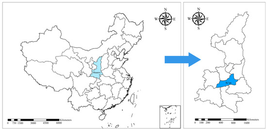
Figure 1.
Location of Xi’an City.
The data used in this study were from the China Urban Statistical Yearbook (2011–2021), the Shaanxi Statistical Yearbook (2011–2021), the Xi’an Statistical Yearbook (2011–2021), the China Environmental Yearbook (2011–2021), and the yearbooks of districts and counties within Xi’an (2011–2021).
2.2. Research Methods
2.2.1. Entropy Weight Method
According to the definition of information entropy, entropy can be used to evaluate the dispersion degree of an index. The larger the information entropy, the greater the dispersion degree of the index, and the more significant the impact (i.e., weight) of the index on comprehensive evaluation [19]. The specific formula of the entropy weight method is as follows:
- (1)
- Data standardization processing
- (2)
- Scheme effect evaluation
2.2.2. EBM Model
The DEA models are divided into radial and non-radial categories and are commonly used to measure efficiency. According to the existing literature, both models have certain shortcomings: the radial models cannot consider the influence of non-radial relaxation, which may overestimate the efficiency value of DMU (Decision Making Units) and lead to measurement deviation [20], as in the CCR model. In contrast, the non-radial models represented by the SBM model are designed to minimize input, thereby discarding different proportions of original input resources, and may lead to an underestimation of the efficiency score of DMU [21]. The EBM model proposed by Tone et al. can effectively combine radial and non-radial methods and then effectively solve the defects of the radial and non-radial models [22]. Based on the EBM model, this study measured the development efficiency of Xi’an and explored the main factors affecting efficiency. The specific linear programming formula of the EBM model is as follows.
Suppose there are n DMUs, m input variables, s expected outputs, and q unexpected outputs; then,
where T* represents the efficiency score of DMUs, which varies from 0 to 1. si−, sr+good, and sp−bad represent the slack and surplus variables for input i, desired output r, and undesired output p, respectively. represents the input weight of item i and is the output weight. ωr+good and ωp−bad represent the expected and unexpected output weights, respectively. Parameter εx stands for radial direction γ and non-radial relaxation sets, and parameter εy stands for radial Ψ and non-radial relaxation sets. εx and εy meet the following conditions: when 0 ≤ εx ≤ 1, 0 ≤ εy ≤ 1, and εx = 0, the EBM model will be simplified to the DEA-CCR model. When εx = εy = 1, it is transformed into the DEA-SBM model.
3. The Construction of Urban Development Models Based on System Dynamics
Professor Jay W. Forrester of the Massachusetts Institute of Technology developed the system dynamics approach, which is an information feedback system used to explore the internal interactions of complex systems, in 1956 [23]. A complex system is a nonlinear composite system comprising multiple subsystems. The urban development process is typically a complex system. System dynamics uses systems thinking to divide a complex system into several subsystems. It analyzes the relationships between subsystems to determine the feedback characteristics and the root cause of the problem from the internal structure to seek system improvement [24].
3.1. System Structure Analysis
The system dynamics model was mainly established to predict the development status of Xi’an in 2021–2025, to a certain extent, and to select an optimal development route by designing a variety of development models for simulation. The urban development model established in this study consisted of three subsystems: the economy, society, and the environment. The subsystems interact with each other and form a dynamic system. System structure analysis is helpful in clarifying the relationships between the three subsystems, which restrict and promote each other and provide support for the construction of the model. The relationships between the subsystems of the urban development model are shown in Figure 2.
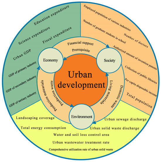
Figure 2.
Subsystem diagram. (Note: The outer circle in the figure is yellow for environmental subsystems, green for economic subsystems, and orange for social subsystems).
3.1.1. Economic Subsystem Analysis
The economic subsystem plays an important role in urban development and needs to fully consider the economic aggregation, growth rate, structure, efficiency, expenditure, and other factors [25,26]. The core variable of economic aggregation is GDP, which is an important indicator for measuring the state and development level of a country or region [27]. Under different economic structures, changes in the proportion of GDP in the three major industries will have an important impact on economic development. The economic growth rate mainly refers to the GDP growth rate, which reflects the vitality of economic development and is an important factor in economic development. Economic development also provides funds for social development, and various social elements, such as culture, education, medical care, and social security, cannot be separated from economic support, which is mainly manifested in various aspects of fiscal expenditure [28]. In addition, various production wastes and harmful gasses generated during economic development pose a threat to the environment [29]. However, with rapid economic development, the funds available for ecological protection are relatively sufficient. Therefore, it is necessary to strengthen ecological protection during active economic development to achieve a balance between them.
3.1.2. Social Subsystem Analysis
The social subsystem comprises several aspects. The most important variable is the total population. Population growth is directly affected by birth rate, mortality, and population base, but it is also indirectly affected by the medical level, living standards, etc. [30]. Additionally, this study comprehensively considered medical treatment, education, culture, science, residents’ lives, and other aspects, specifically the number of doctors, the number of postgraduates in school, public library collections, the number of invention patents granted, per capita disposable income, and other variables. Social development depends on all types of production and living materials provided by the environment, which produces waste [27]. Therefore, human social activities also need to consider the requirements of the environmental carrying capacity.
3.1.3. Environmental Subsystem Analysis
The environmental subsystem includes the total energy consumption, urban waste output, total amount of municipal solid waste, water and soil loss control area, green park area, and other variables. It is an important link in the urban development process, provides the basis for economic and social development, and provides production and living materials for various industries. However, the ecological carrying capacity must be considered in this process, and excessive development will lead to an environmental imbalance [31].
3.2. System Dynamics Model
3.2.1. System Variables and Model Establishment
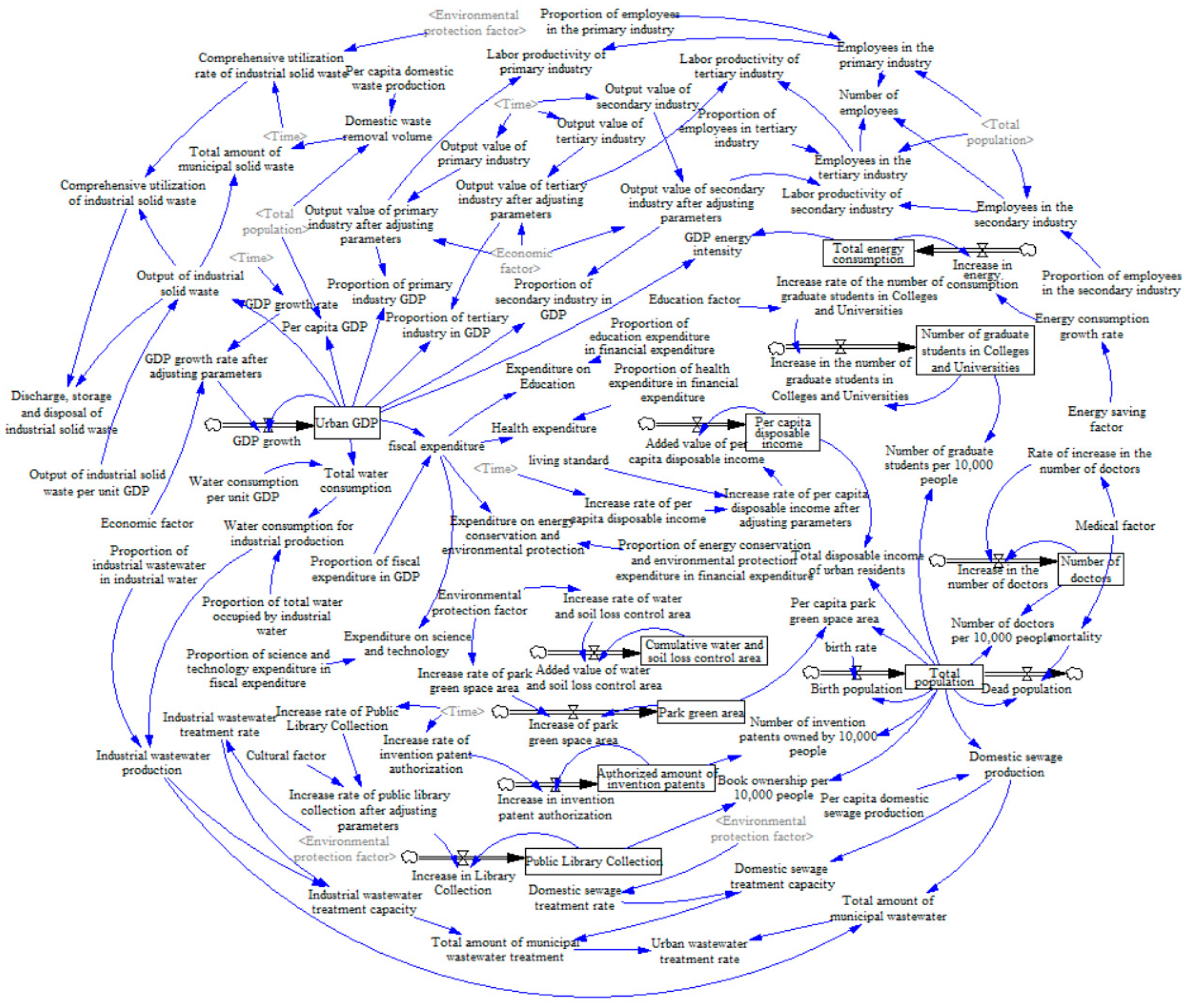
The system dynamics model originates from the theory of system science, and along with the continuous development and improvement of theoretical knowledge as well as socio-economic progress, the scope of application is gradually expanding. Subsequently, Forrester extended industrial dynamics [32] to the field of urban dynamics [33] to analyze correlations between variables and feedback mechanisms between systems. This study will construct a system dynamics model of the three subsystems—economic, social, and environmental—that balances efficiency and effectiveness. Using Vensim PLE x32 software, the administrative part of the study area was used as the system boundary, and the simulation period was 2010–2025 with a simulation step of 1 year, from which the optimal plan for urban development was selected. The study of urban development patterns using a system dynamics approach can be divided into the following stages: (1) Sorting out the systemic relationship of urban development in Xi’an and analyzing the three subsystems of economy, society, and environment in Xi’an, as well as the interrelationships among them; (2) Establishing a system dynamics model; (3) Conducting scenario modeling and simulation of urban development in Xi’an; and (4) Based on the test results of the SD model, analyzing the urban development patterns under different plans and judging from them the optimal plan that meets the urban development of Xi’an. The main causal relationships of the SD model are shown in Figure 3, and the stocks and flows diagram is shown in Figure 4.
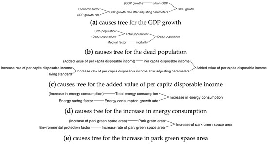
Figure 3.
Causes trees for the main system variables.
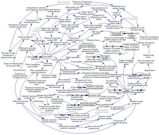
Figure 4.
The stocks and flows diagram. (Note: The tails of the arrows in the figure are the causes and the arrows are the results).
- (1)
- Causality analysis
System modeling is based on causality analysis. By analyzing the interactions between the variables in the system, the causal relationship can be determined, which can be expressed by the causes tree. In the economic subsystem, urban GDP was related to GDP growth, which in turn was influenced by GDP growth rate and economic control factors. In the social subsystem, the total population was related to the birth and death population, and the death population was affected by the mortality rate and the level of medical services; per capita, disposable income was related to the added value of disposable income, which in turn was affected by the increase rate of per capita disposable income and the living standards. In the environmental subsystem, total energy consumption was related to the increase in energy consumption, which in turn was affected by the energy consumption growth rate and energy saving factor; the green park area was affected by the increase rate of the park green space area and the environmental protection factor.
- (2)
- Variable selection and setting
There are four variables in system dynamics: level, rate, auxiliary, and constant [34]. The level variable is a state variable that represents the cumulative level of some physical quantities over time, such as the total population. The rate variable is mainly used to display the increment of the value of the horizontal variable over time, which is a differential variable acting on the horizontal variable, such as population increment. The constant variable is a quantity that remains constant throughout the system, such as various control factors in the system. The remaining variables are auxiliary variables, which are used to connect different stocks and flows in various forms [35]. Ten level variables were designed in this study: urban GDP, total energy consumption, cumulative soil erosion control area, number of postgraduates in school, number of doctors, green park area, number of invention patents granted, public library collection, total population, and per capita disposable income.
- (3)
- Parameter settings
After defining the system structure and related variables, it is first necessary to assign values to each variable. We selected the 2010 data as the basic data, and assigned the initial values of ten horizontal variables and some constant variables. Second, the functional relationship of each variable should be considered, including the basic relationship, regression, tabular, and logical relationship functions [36]. For variables with direct relationships, the functional relationship is generally assigned directly, such as through addition, subtraction, multiplication and division; for variables with clear mathematical relationships, that is, when a variable changes with one or more other variables and presents clear mathematical laws, functional relationships can be obtained through univariate or multivariate regression; for variables with complex nonlinear relationships, table functions can be used for assignment, usually in the form of charts. The logic function includes the selection of maximum and minimum values and conditional judgment. For variables affected by many factors that reflect different characteristics under different conditions, the logic function expression may be used. The variable formulae in the model are listed in Table 1.

Table 1.
Partial variable formulas in the model.
3.2.2. Model Validation
After establishing the system dynamics model, the model should be tested to determine if the model is correct and if it meets certain criteria to ensure the accuracy and validity of the model. Usually, SD model tests include four main types: intuitive tests, operational tests, historical tests, and stability tests. For the theoretical testing of the model, first of all, this paper constructed a systematic simulation model of urban development in Xi’an, which covered three main aspects, namely economic, social, and environmental aspects. Secondly, the data source of this paper is reliable and can reflect the real urban development level of Xi’an, which is of good practical significance. Based on the above, the model passes the theoretical test.
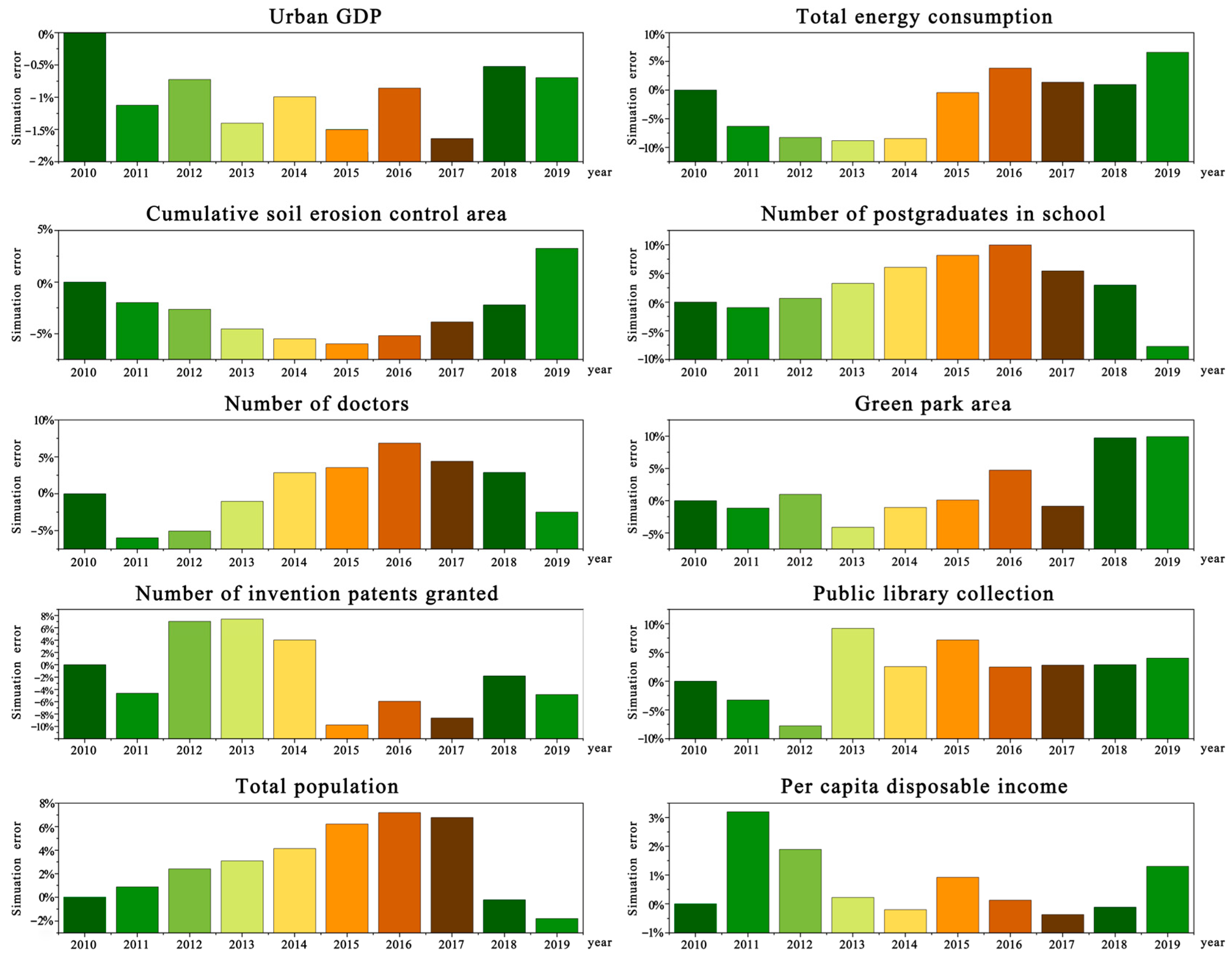
For the historical test, this paper chose the data of Xi’an City from 2011 to 2019 to ensure the validity of the model. A historical test was used to judge whether the model was consistent with the real situation, which was the premise for the model’s simulation and prediction ability. The historical test for this model was the comparison between the simulated and actual values after the model had been run. If the error between the two values was within a certain range, it was considered acceptable, indicating that the model had a certain degree of credibility and could be used for subsequent research [37]. Because the effects of extreme situations such as earthquakes and epidemics are difficult to quantify and do not conform to the formulas already set up by the model, they are not taken into account in this study, and only simulations obtained by evolving according to past trends are considered. The error test results, with the comparison of the simulation data with the actual data, are shown in Figure 5. The simulation errors of all state variables within ten years were less than ±10%, which indicates that the model has a good simulation ability and can be used to carry out research into the urban development model.

Figure 5.
Indicator error diagram.
To ensure that the model has a certain degree of sensitivity and stability, this paper carried out a stability test on the model and selected one year and half a year as the simulation steps of this paper, i.e., DT = 1, DT = 0.5. The results found that the model can more realistically reflect the relationship between the various subsystems, and the test results proved that the model has a certain degree of stability.
In summary, the model can be used for the subsequent urban development scenario design and simulation analysis.
3.3. Urban Development Scenario Design and Simulation
This study took 2021–2025 as the simulation period. On the one hand, it is of great significance to examine 2021–2025, as the implementation years of the Fourteenth Five-Year Plan of China. In addition, the Xi’an Metropolitan Area Development Plan (2022) clearly states that the radiation-driving capacity of Xi’an should be further improved by 2025. In contrast, considering that the uncontrollable factors of the system increase with time, it may be difficult to obtain accurate values for a long simulation cycle; therefore, the simulation cycle must be set to as short as possible, and a five-year period is appropriate.
To explore the impact of the three subsystems on the development of Xi’an under different scenarios more deeply, seven control factors were added based on the system dynamics model. Eight development plans were designed by varying the control factor values, including the current (P1), economic (P2), social (P3), environmental (P4), economic–social (P5), economic–environmental (P6), social–environmental (P7), and comprehensive development (P8) plans, and the development situation of Xi’an in 2021–2025 was simulated.
The control factors act directly on some variables in the system dynamics, changing them proportionally, and then indirectly affect the entire system. The simulation values under different plans can be obtained by combining the values of different control factors. The seven control factors are economic, energy-saving, environmental protection, life, medical, cultural, and educational factors. Among them, the economic factor belongs to the economic subsystem, the energy-saving and environmental protection factors belong to the environmental subsystem, and the life, medical treatment, cultural, and educational factors belong to the social subsystem. Although the number of control factors in the three subsystems is different, the number of variables controlled by the different control factors is also different, and it was verified that the degree of influence in each subsystem was basically the same. Among them, some of the variables directly affected by economic, energy-saving, environmental protection, life, medical, cultural, and educational factors included the GDP growth rate and output value of the three industries; energy consumption and growth rate; domestic sewage treatment, industrial solid waste comprehensive utilization, and industrial wastewater treatment rates; per capita disposable income; number of doctors and mortality; public library collection; and the number of postgraduates in school, respectively.
The changes in the control factors should not be too large or small. Changes that are too small will lead to insignificant changes and a lack of discrimination, whereas those that are too large will cause the simulation value to deviate from the actual value. The change in the control factors was moderate when it was within 10–30%, after debugging the factors many times. The values of the control factors are listed in Table 2.
Table 2.
Control factors of different plans.
4. Evaluation of Urban Development Model Based on Entropy Weight Method and DEA-EBM
4.1. Construction of the Indicator System
To ensure the consistency of the effect and efficiency evaluation, only one index system was constructed in this study. The effect was used to evaluate external performance; therefore, the selected indicators were only output indicators. The efficiency was used to analyze the system configuration and needed to consider input and output indicators simultaneously. Therefore, there was a difference between the effect and efficiency indicator systems regarding whether input indicators were required.
To understand the essential requirements and external characteristics of urban development, considering the availability, quantification, and reliability of statistical data, as well as the fairness of the number of indicators of the three subsystems, four indicators were selected from each subsystem of system dynamics, and the values of all indicators were obtained from the above system dynamics simulation. The economic, social, and environmental indicators included the economic level, structure, efficiency, and growth; medical health, higher education, cultural publicity, and people’s lives; and the greening of the city, environmental governance, wastewater treatment, and waste disposal. Subsequently, considering economic and environmental inputs, this study selected the financial expenditure and total energy consumption as DEA input indicators to form a complete indicator system.
In evaluating the effects, this study does not set non-desired outputs due to the need to ensure the harmonization of the before-and-after indicator system, as well as for fairness considerations in the number of indicators for the three major subsystems. In addition, because the DEA method is limited to the number of indicators, the number of indicators needs to be reduced as much as possible, and therefore the numerical values of the indicators need to be processed during the calculation. The data of the secondary indicators within the subsystem are standardized, processed, and summed up as the values of the primary output indicators, which are used as the basic data for the DEA calculation. The final input indicators were fiscal expenditure (I1) and total energy consumption (I2), and the final output indicators were economic output (O1), social output (O2), and environmental output (O3). The standardized DEA calculation data are presented in Table 3.
Table 3.
DEA calculation data.
4.2. Weight Calculation
When using the effect evaluation, considering that the economic, social, and environmental subsystems may have different degrees of influence on urban development, as well as the degree of impact of the indicators within the subsystems, the entropy weight method was used to calculate the weight of each indicator and evaluate the effect of each plan. According to the definition of the entropy weight method, the weight of each index was calculated using Equations (1)–(6). The top three weighted indicators are the GDP growth rate, number of doctors (public library collection), and green park area, with weights of 0.087, 0.091, and 0.098, respectively. As far as the subsystems are concerned, the social subsystem has a higher weight of 0.356 and the environmental subsystem and the economic subsystem both have weights of 0.322, which is basically consistent with reality. The effectiveness and efficiency evaluation index systems are presented in Table 4.
Table 4.
The effectiveness and efficiency evaluation index systems.
5. Results and Discussion
5.1. Analysis of Urban Development Effect
5.1.1. Scheme Analysis
Based on the system dynamics simulation of the eight plans, the urban development effect was evaluated according to Equation (6), with the simulation values of each indicator in the indicator system in 2021–2025 as the basic data. These scores are presented in Table 5.
Table 5.
Score of each plan.
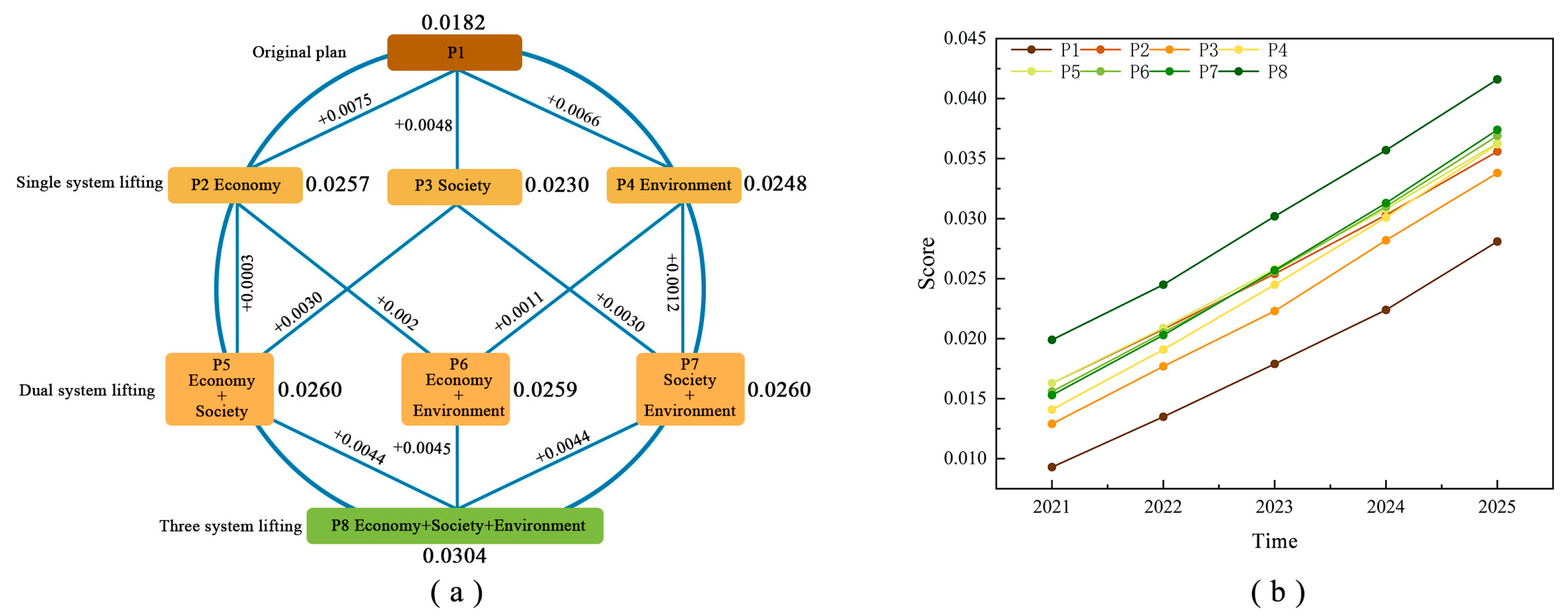
The average scores and evolution trends of the eight plans over five years are shown in Figure 6a. The average scores decreased in the order of P8 > P7 > P5 > P6 > P2 > P4 > P3 > P1. From the score ranking and grouping, based on the original plan, increasing investment will have a positive impact on regional development. This result confirms the concept of “effect”, that is, the effect is an evaluation of the system’s external performance and development level. Increasing the input makes more resources available for distribution, and the system output is optimized, which is reflected in the improvement in the development level and better development effect.
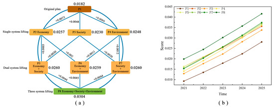
Figure 6.
Evaluation scores and evolution of each plan. (Figure (a) represents the average scores and evolution trends over the five years of the program, and figure (b) represents the comprehensive scores of the programs over the five years.).
According to their ranking, the eight plans could be divided into four groups. The first group was P8, which had the highest score, with an average of 0.0304 in five years, an increase of 66.88% compared with the original plan. The second group had the second-highest score, and this was the plan to improve the twin subsystems, including P7, P5, and P6. The average scores were 0.0260, 0.0260, and 0.0259, respectively, which were 42.73%, 42.73%, and 42.33% higher than the original plan. The third group was the plan to improve the single subsystem, including P2, P4, and P3. The average scores were 0.0257, 0.0248, and 0.0230, respectively, 40.83%, 36.04%, and 26.14% higher than those of the original plan. The fourth group had the lowest score of 0.0182, which was P1 of the original plan.
According to the grouping, the effect of the single-system improvement plans was relatively low, with an average increase of 34.34% in P2, P4, and P3 compared with the original plan. This may be because the single-system improvement made the development of this subsystem more prominent, while other subsystems were in a relatively backward position, with low overall coordination, and the interaction effect between systems was not obvious. In the double-system upgrading, P7, P5, and P6 were improved by 42.63% on average compared with the original plan. The overall coordination of the system was good, and the interaction between the two promoted subsystems played a role in promoting overall development. For the comprehensive development plan, with three systems simultaneously promoted, although each subsystem was promoted less, the mutual promotion among subsystems optimized the overall development effect. The results are similar to those of Dong and Shang’s [61] study on the development of western urban agglomeration, which includes Xi’an City; that is, in the five years after 2021, a simultaneous improvement in the key indicators of the economic, social, and environmental subsystems to an appropriate degree could lead to a balanced development of the subsystems and the highest level of urban development.
The comprehensive scores for each plan over five years are shown in Figure 6b. The scores from P1 to P8 increased by 203.20%, 118.34%, 161.29%, 156.84%, 122.35%, 136.16%, 145.38%, and 109.08%, respectively, in the five years, with similar growth rates and consistent changes in trends over time. This may be because, although the improvement ideas of each plan were different, the setting of the control factors ensured that the overall range of the change was similar. The effect of growth rate mainly reflected the urban development capacity, which was closely related to the characteristics of the city. Owing to the emphasis on balanced development in recent years, Xi’an has had a relatively reasonable industrial structure and a good development foundation; hence, the potential for development is enormous. The effects of different development plans had different levels, but this would not greatly affect future development prospects; thus, the change trend of the effect evaluation of all plans in 2021–2025 was relatively consistent.
5.1.2. Subsystem Analysis
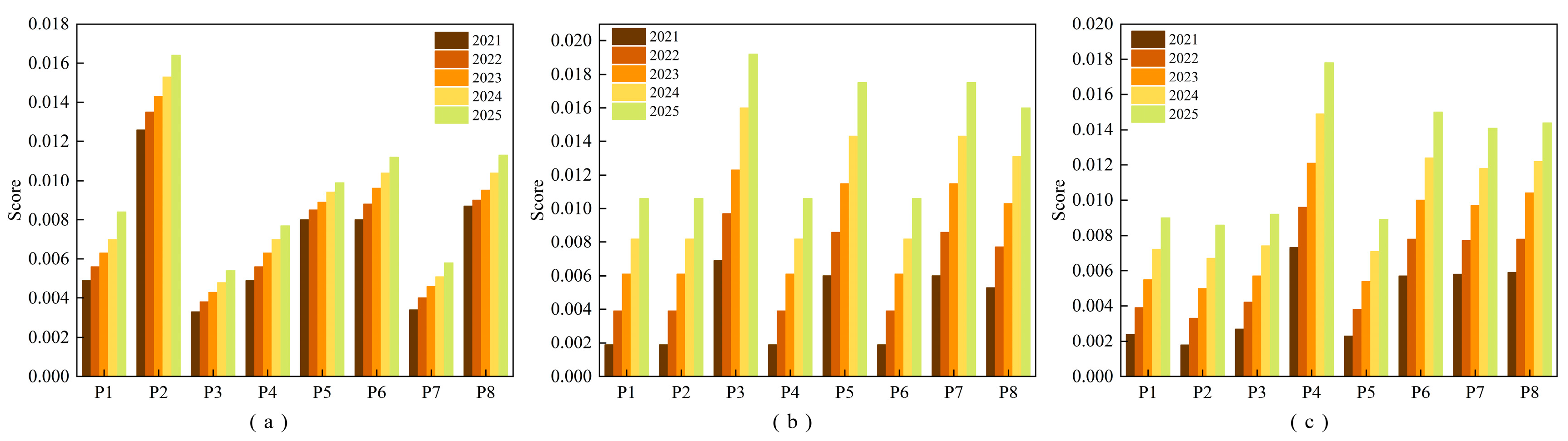
Figure 7 shows the annual scores of the three subsystems of economy, society, and environment for the eight plans, and Table 6 shows the average scores of each plan.

Figure 7.
Scores of three subsystems in each year. ((a–c) represent the annual scores of the economy, society, and environment subsystems for each of the eight plans.).
Table 6.
Average scores of subsystems over five years.
By analyzing the data, it was found that the contribution values of the three subsystems of economy, society, and environment under the current situation were not significantly different. The highest average score for the economic subsystem was that of P2 (0.01446), the highest score for the social subsystem was that of P3 (0.01282), and the highest score for the environmental subsystem was that of P4 (0.0123). The highest score was consistent with the actual situation. P2, P3, and P4 were all single-system upgrading plans, and the corresponding subsystem had the largest improvement range; thus, it achieved the highest score.
At the same time, although the single-system improvement plan had an obvious effect on the improvement of the response subsystem, it was obtained at the expense of the scores of other subsystems, such as those of the social subsystem of P2 (0.00601), economic subsystem of P3 (0.00432), and economic subsystem of P4 (0.00628), which were lower than those the original plan. In addition, the promotion of dual systems also reduced the score of the unimproved subsystems, such as P5’s environmental subsystem (0.0054), P6’s social subsystem (0.00588), and P7’s economic subsystem (0.00458). Only P8 achieved a simultaneous improvement in the economic, social, and environmental scores. It can be seen that the comprehensive development plan achieved coordination and symbiosis of the economy, society, and environment, reduced the mutual inhibition between the three subsystems, and achieved optimal development.
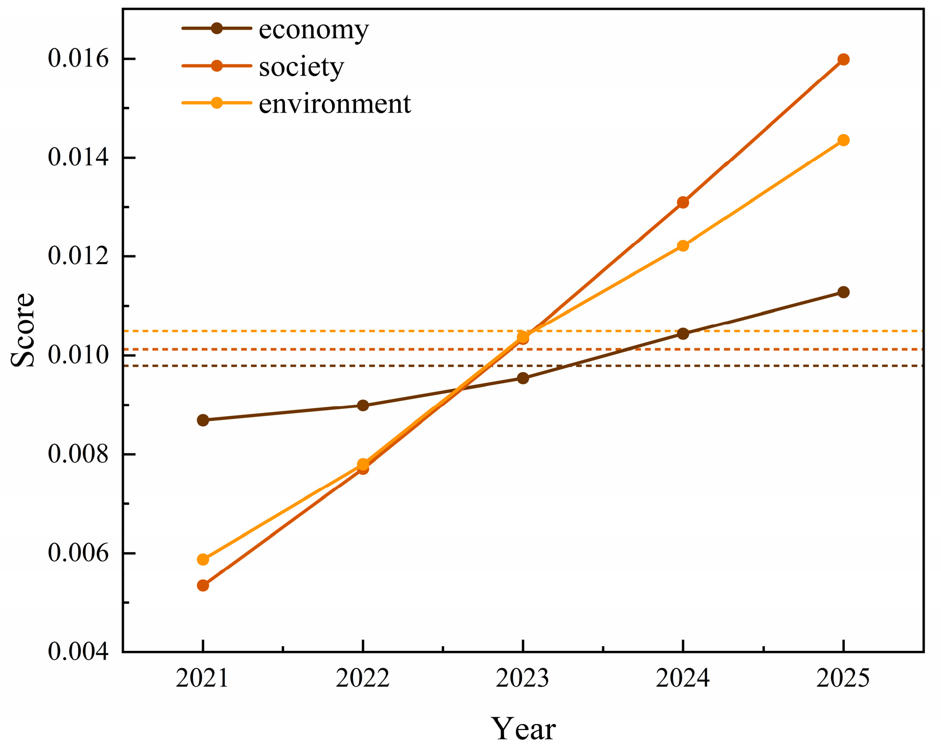
As P8 was a coordinated development plan with the highest score, its score was disassembled to analyze the contribution of the three subsystems to the effect of urban coordinated development. Figure 8 shows the scores of each subsystem of P8 from 2021 to 2025. It can be seen that the economic subsystem grew slowly in five years, with a growth rate of 29.89%. The scores of the social and environmental subsystems experienced significant growth, with rates of 201.89% and 144.07%, respectively. That is, under P8, each unit of economic growth could bring about seven units of social growth and five units of environmental growth. The economic subsystem had the highest score in the first two years, but the growth rate was slow, resulting in the lowest average score, indicating that economic improvement played a catalytic role and achieved better results in the short term. However, it is not sufficient to rely solely on economic development. The more important role of economic subsystem improvement is to enhance support for other subsystems, which requires the combination of economic improvement and the improvement of other systems so that society and the environment can be better developed.

Figure 8.
Subsystem scores of P8.
5.2. Analysis of Urban Development Efficiency
5.2.1. Scheme Analysis
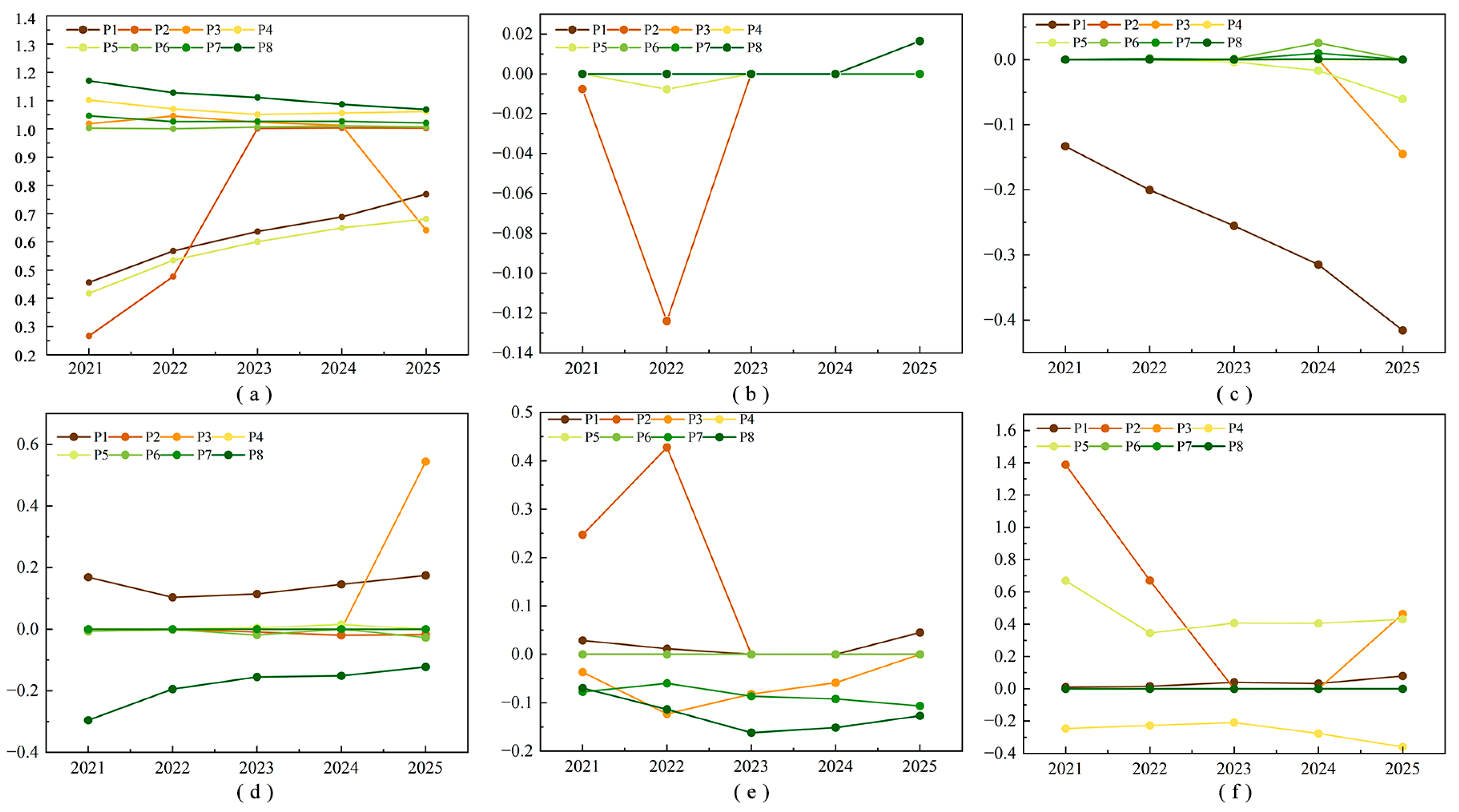
Based on standardized DEA data, this study used the MAX-DEA 5.2 software and a super-efficiency EBM model to measure urban development efficiency. Figure 9a shows the changes in the comprehensive efficiency of the eight plans from 2021 to 2025. The development trend of the eight plans’ efficiency values could be roughly divided into four categories: stable, rapid growth, slow growth, and sharp reduction.
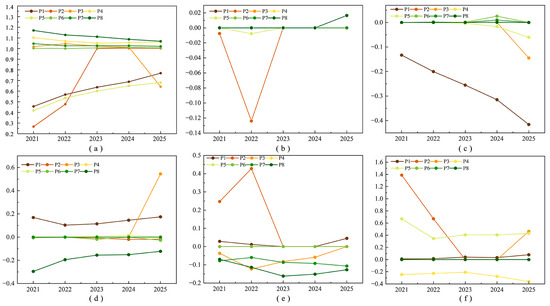
Figure 9.
Efficiency score of each plan and slack of each index. (Note: (a) represents the change in combined efficiency of the eight programs from 2021 to 2025. (b) represents Economic input; (c) represents Resource input; (d) represents Economic output; (e) represents Social output; (f) represents Environmental output).
P4, P6, P7, and P8 were stable, and the comprehensive efficiency decreased in the order of P8 > P4 > P7 > P6. The DEA efficiencies of these four plans were in a stable state, and all of them were greater than 1 within five years, demonstrating the DEA’s effectiveness and indicating that these plans reached the ideal level of input and output, fully utilized resources, and had no shortage of input redundancy and output, indicating that they could be good alternative plans. According to the specific contents of the plans, it can be seen that the four effective DEA plans all included the idea of improving the environmental subsystem. It can be seen that the environmental subsystem was an important link in achieving efficiency standards, which could ensure the full use of economic and resource inputs.
P2 was of the rapid-growth type. Its efficiency was only 0.27 in 2021, but it reached DEA efficiency and maintained stability after two years. This shows that the economic subsystem was upgraded independently under the current development situation, and that there was a situation of excessive economic input. With the further development of the economy, the output further increased, and the increase in output speed rapidly improved, gradually reaching a balance between input and output. This shows that there is still some room for progress in the current economic situation, and further development of the economic level can improve the optimization of the system element configuration.
P1 and P5 were of the slow-growth types. P1 was the original plan, and its low efficiency indicated that the current resource allocation in Xi’an was unbalanced. Over time, the efficiency value gradually increased, but the speed was slow, indicating that, according to the current situation, a better configuration scheme could be obtained; however, it would take a long time, so it would be necessary to upgrade the system. The efficiency of P5 was even lower than that of P1 in each year, which may be because economic and social development take the environment as the cost, so the consumption of the environment was the largest, rendering the entire system configuration unreasonable and the development direction problematic.
P3 was of the sharp-reduction type. Its efficiency reached DEA efficiency in 2021–2024, but decreased to 0.64 in 2025; that is, the current output level could be obtained with only 64% of the input. This indicates that, under the development situation of P3, the continued improvement of the social subsystem in 2025 would cause the input to continue to increase; however, the output would have little effect. This also indicates that the social subsystem developed to a high level by 2025 under this plan, and the continued improvement was of little significance.
5.2.2. Input and Output Analysis
Figure 9b–f show the slack variables for economic input, resource input, economic output, social output, and environmental output, respectively. The slack quantity represented the distance between the actual input (output) and effective input (output). For the input index, a positive slack indicated that the investment scale could be further improved, while a negative slack indicated that the investment was excessive and there was waste. For the output index, a positive slack meant that there was insufficient output, while a negative slack meant that the actual output was greater than the effective output.
- (1)
- Economic input
As shown in Figure 9b, the slack of economic input in P1, P3, P4, P6, and P7 was zero, indicating that the economic input in these five plans was ideal, there was no redundancy, and the scale was optimal. P2 had economic input redundancy in 2021 and 2022, indicating that the plan’s promotion of the economic subsystem was somewhat excessive in these two years. The rapid increase in economic output in the following three years consumed excessive economic input, reducing the slack in economic input to 0. The slack of P8 was positive in 2025, which could appropriately expand the scale of economic input and obtain greater output to ensure efficiency.
- (2)
- Resource input
As shown in Figure 9c, the slack of the resource inputs in P2 and P4 over five years was 0, indicating that the energy input in these two plans was fully utilized. P1 had resource input redundancy in five years, whereas P3 and P5 had input redundancy in some years, showing that there was still room for improvement in the utilization of resources, and that the improvement of the economic and social subsystems could improve the efficiency of resource utilization to a certain extent. However, there was no redundancy among the remaining plans. P6, P7, and P8 could further improve the resource utilization capacity, indicating that the improvement in the environmental subsystem could play a vital role in resource utilization.
- (3)
- Economic output
As shown in Figure 9d, P1 had insufficient economic output, indicating that there was still room for progress in economic output in terms of the current development situation, and further proving that the level of economic development could improve development efficiency. P3 and P5 also had insufficient economic output, but compared with P1, the situation of insufficient output was alleviated, indicating that social development would promote economic output to a certain extent and weaken its shortage. Other plans, including the improvement of environmental subsystems, had no insufficient economic output, indicating that environmental development plays a supporting and promoting role in economic development.
- (4)
- Social output
As shown in Figure 9e, only P1 and P2 had insufficient social output in some years, indicating that social output still needed to be improved under the current development situation, while the economic and environmental subsystems could promote social output, and the effect of environmental improvement would be greater than that of economic improvement.
- (5)
- Environmental output:
As shown in Figure 9f, P1, P2, P3, and P5 all had insufficient environmental outputs, indicating that the environmental subsystem was the basis of the economic and social subsystems and guaranteed the efficiency of the entire system. Economic and societal development are based on the environment, causing environmental damage to a certain extent. Therefore, during urban development, special attention must be paid to environmental improvement.
6. Conclusions
Combining system dynamics, the entropy weight method, and DEA, this study not only explored the relationship between internal factors during urban development, but also provided a method for urban development evaluation considering both effect and efficiency. Through the construction of a system dynamics model, this study explored the dynamic process of urban development in depth, as well as the complex interaction and feedback mechanisms among the economy, society, and the environment. In combination with the actual development situation of Xi’an City, eight development plans were proposed and the variable values of each plan for 2021–2025 were simulated using the system dynamics model. Based on the simulation values, the entropy weight method and DEA were used to calculate the development effect and efficiency, and the advantages and disadvantages of each plan were compared. The calculation results show that (1) the development effect of P8 ranked first, and it also reached DEA effectiveness in each year, meaning it can be used as the best plan for the future development of Xi’an City. The effect scores of P6 and P7 were at a higher level, and they also reached DEA effectiveness in each year, and could be used as an alternative plan. (2) From the perspective of effect, the mode of comprehensive development can make subsystems promote each other to improve the development level, while upgrading a subsystem alone may sacrifice the subsystem that has not been upgraded, thereby affecting the overall development level. (3) From the perspective of efficiency, four effective DEA plans all included the idea of improving the environmental subsystem, indicating that the environmental subsystem is the foundation of economy and society, and also the guarantee of the efficiency of the whole system. Therefore, in the process of urban development, special attention must be paid to environmental improvement.
The calculation results of this study were relatively ideal. The plan with the best effect was also the plan with the best efficiency; therefore, no further analysis was carried out. Subsequent studies can be further analyzed by introducing methods such as group decision making. Moreover, this study only focused on the city of Xi’an. The study area can be extended to more diverse cities or regions in the follow-up studies to improve the generalizability.
Author Contributions
Conceptualization, L.Y.; methodology, L.Y., Y.M. and K.L.; software, Y.M. and K.L.; validation, L.Y.; formal analysis, Y.M. and K.L.; investigation, Y.M. and K.L.; resources, L.Y.; data curation, L.Y., Y.M. and K.L.; writing—original draft preparation, Y.M. and K.L.; writing—review and editing, L.Y.; visualization, Y.M. and K.L.; supervision, L.Y.; project administration, L.Y.; funding acquisition, L.Y. All authors have read and agreed to the published version of the manuscript.
Funding
This research was funded by [the National Natural Science Foundation of China (NSFC) Youth Science Fund Project] grant number [52209034]. And the Scientific Research Program Funded by the Shaanxi Provincial Education Department (Program No. 20JT052).
Data Availability Statement
The data are available on request from the corresponding author.
Conflicts of Interest
Author K.L. was employed by the company PowerChina Beijing Engineering Corporation Limited. The authors declare that they have no known competing financial interests or personal relationships that could have appeared to influence the work reported in this paper.
References
- Song, C.; Wu, L.; Xie, Y.; He, J.; Chen, X.; Wang, T.; Lin, Y.; Jin, T.; Wang, A.; Liu, Y.; et al. Air Pollution in China: Status and Spatiotemporal Variations. Environ. Pollut. 2017, 227, 334–347. [Google Scholar] [CrossRef] [PubMed]
- Choy, L.H.T.; Li, V.J. The Role of Higher Education in China’s Inclusive Urbanization. Cities 2017, 60, 504–510. [Google Scholar] [CrossRef]
- Dong, L.; Longwu, L.; Zhenbo, W.; Liangkan, C.; Faming, Z. Exploration of Coupling Effects in the Economy–Society–Environment System in Urban Areas: Case Study of the Yangtze River Delta Urban Agglomeration. Ecol. Indic. 2021, 128, 107858. [Google Scholar] [CrossRef]
- Jing, Z.; Wang, J. Sustainable Development Evaluation of the Society–Economy–Environment in a Resource-Based City of China: A Complex Network Approach. J. Clean. Prod. 2020, 263, 121510. [Google Scholar] [CrossRef]
- Tan, F.; Lu, Z. Study on the Interaction and Relation of Society, Economy and Environment Based on PCA–VAR Model: As a Case Study of the Bohai Rim Region, China. Ecol. Indic. 2015, 48, 31–40. [Google Scholar] [CrossRef]
- Bahtebay, J.; Zhang, F.; Ariken, M.; Chan, N.W.; Tan, M.L. Evaluation of the Coordinated Development of Urbanization-Resources-Environment from the Incremental Perspective of Xinjiang, China. J. Clean. Prod. 2021, 325, 129309. [Google Scholar] [CrossRef]
- Shen, L.; Huang, Y.; Huang, Z.; Lou, Y.; Ye, G.; Wong, S.-W. Improved Coupling Analysis on the Coordination between Socio-Economy and Carbon Emission. Ecol. Indic. 2018, 94, 357–366. [Google Scholar] [CrossRef]
- Hao, L.; Yu, J.; Du, C.; Wang, P. A Policy Support Framework for the Balanced Development of Economy-Society-Water in the Beijing-Tianjin-Hebei Urban Agglomeration. J. Clean. Prod. 2022, 374, 134009. [Google Scholar] [CrossRef]
- Li, W.; Bao, L.; Wang, L.; Li, Y.; Mai, X. Comparative Evaluation of Global Low-Carbon Urban Transport. Technol. Forecast. Soc. Chang. 2019, 143, 14–26. [Google Scholar] [CrossRef]
- Jia, B.; Zhou, J.; Zhang, Y.; Tian, M.; He, Z.; Ding, X. System Dynamics Model for the Coevolution of Coupled Water Supply–Power Generation–Environment Systems: Upper Yangtze River Basin, China. J. Hydrol. 2021, 593, 125892. [Google Scholar] [CrossRef]
- Guo, H.; Yang, C.; Liu, X.; Li, Y.; Meng, Q. Simulation Evaluation of Urban Low-Carbon Competitiveness of Cities within Wuhan City Circle in China. Sustain. Cities Soc. 2018, 42, 688–701. [Google Scholar] [CrossRef]
- Li, R.; Wu, Q.; Jinjin, Z.; Wen, Y.; Li, Q. Effects of Land Use Change of Sloping Farmland on Characteristic of Soil Erosion Resistance in Typical Karst Mountainous Areas of Southwestern China. Pol. J. Environ. Stud. 2019, 28, 2707–2716. [Google Scholar] [CrossRef] [PubMed]
- Jiang, J. China’s Urban Residential Carbon Emission and Energy Efficiency Policy. Energy 2016, 109, 866–875. [Google Scholar] [CrossRef]
- Cheng, M.; Lu, Y. Investment Efficiency of Urban Infrastructure Systems: Empirical Measurement and Implications for China. Habitat Int. 2017, 70, 91–102. [Google Scholar] [CrossRef]
- Chen, J.; Zhang, W.; Song, L.; Wang, Y. The Coupling Effect between Economic Development and the Urban Ecological Environment in Shanghai Port. Sci. Total Environ. 2022, 841, 156734. [Google Scholar] [CrossRef] [PubMed]
- Li, J.; Shi, J.; Duan, K.; Li, H.; Zhang, Y.; Xu, Q. Efficiency of China’s Urban Development under Carbon Emission Constraints: A City-Level Analysis. Phys. Chem. Earth Parts A/B/C 2022, 127, 103182. [Google Scholar] [CrossRef]
- Guo, J.; Ma, S.; Li, X. Exploring the Differences of Sustainable Urban Development Levels from the Perspective of Multivariate Functional Data Analysis: A Case Study of 33 Cities in China. Sustainability 2022, 14, 12918. [Google Scholar] [CrossRef]
- Yang, Q.; Sun, Z.; Zhang, H. Assessment of Urban Green Development Efficiency Based on Three-Stage DEA: A Case Study from China’s Yangtze River Delta. Sustainability 2022, 14, 12076. [Google Scholar] [CrossRef]
- Huang, W.; Shuai, B.; Sun, Y.; Wang, Y.; Antwi, E. Using Entropy-TOPSIS Method to Evaluate Urban Rail Transit System Operation Performance: The China Case. Transp. Res. A Policy Pract. 2018, 111, 292–303. [Google Scholar] [CrossRef]
- Wu, Z.; Liu, T.; Xia, M.; Zeng, T. Sustainable Livelihood Security in the Poyang Lake Ecological Economic Zone: Identifying Spatial-Temporal Pattern and Constraints. Appl. Geogr. 2021, 135, 102553. [Google Scholar] [CrossRef]
- Ren, F.; Tian, Z.; Liu, J.; Shen, Y. Analysis of CO2 Emission Reduction Contribution and Efficiency of China’s Solar Photovoltaic Industry: Based on Input-Output Perspective. Energy 2020, 199, 117493. [Google Scholar] [CrossRef]
- Zeng, P.; Wei, X. Measurement and Convergence of Transportation Industry Total Factor Energy Efficiency in China. Alex. Eng. J. 2021, 60, 4267–4274. [Google Scholar] [CrossRef]
- Papachristos, G. System Dynamics Modelling and Simulation for Sociotechnical Transitions Research. Environ. Innov. Soc. Transit. 2019, 31, 248–261. [Google Scholar] [CrossRef]
- Bugalia, N.; Maemura, Y.; Ozawa, K. A System Dynamics Model for Near-Miss Reporting in Complex Systems. Saf. Sci. 2021, 142, 105368. [Google Scholar] [CrossRef]
- Zhang, Y.; Mao, W.; Zhang, B. Distortion of Government Behaviour under Target Constraints: Economic Growth Target and Urban Sprawl in China. Cities 2022, 131, 104009. [Google Scholar] [CrossRef]
- Yin, X.; Xu, Z. An Empirical Analysis of the Coupling and Coordinative Development of China’s Green Finance and Economic Growth. Resour. Policy 2022, 75, 102476. [Google Scholar] [CrossRef]
- Weng, Q.; Lian, H.; Qin, Q. Spatial Disparities of the Coupling Coordinated Development among the Economy, Environment and Society across China’s Regions. Ecol. Indic. 2022, 143, 109364. [Google Scholar] [CrossRef]
- Gan, L.; Yang, X.; Chen, L.; Lev, B.; Lv, Y. Optimization Path of Economy-Society-Ecology System Orienting Industrial Structure Adjustment: Evidence from Sichuan Province in China. Ecol. Indic. 2022, 144, 109479. [Google Scholar] [CrossRef]
- Zhang, H.; Wang, Y.; Wang, C.; Yang, J.; Yang, S. Coupling Analysis of Environment and Economy Based on the Changes of Ecosystem Service Value. Ecol. Indic. 2022, 144, 109524. [Google Scholar] [CrossRef]
- Liu, J.; Tian, Y.; Huang, K.; Yi, T. Spatial-Temporal Differentiation of the Coupling Coordinated Development of Regional Energy-Economy-Ecology System: A Case Study of the Yangtze River Economic Belt. Ecol. Indic. 2021, 124, 107394. [Google Scholar] [CrossRef]
- Fan, Y.; Fang, C.; Zhang, Q. Coupling Coordinated Development between Social Economy and Ecological Environment in Chinese Provincial Capital Cities-Assessment and Policy Implications. J. Clean. Prod. 2019, 229, 289–298. [Google Scholar] [CrossRef]
- Forrester, J.W. Industrial Dynamics. J. Oper. Res. Soc. 1997, 48, 1037–1041. [Google Scholar] [CrossRef]
- Forrester, J.W. Urban Dynamics. IMR Ind. Manag. Rev. (Pre-1986) 1970, 11, 67. [Google Scholar] [CrossRef]
- Kotagodahetti, R.; Hewage, K.; Karunathilake, H.; Sadiq, R. Long-Term Feasibility of Carbon Capturing in Community Energy Systems: A System Dynamics-Based Evaluation. J. Clean. Prod. 2022, 377, 134460. [Google Scholar] [CrossRef]
- Wang, G.; Yuan, M.; Xu, H. The Impact of Subsidy and Preferential Tax Policies on Mobile Phone Recycling: A System Dynamics Model Analysis. Waste Manag. 2022, 152, 6–16. [Google Scholar] [CrossRef]
- Liu, B.; Qin, X.; Zhang, F. System-Dynamics-Based Scenario Simulation and Prediction of Water Carrying Capacity for China. Sustain. Cities Soc. 2022, 82, 103912. [Google Scholar] [CrossRef]
- Liu, G.; Xu, Y.; Ge, W.; Yang, X.; Su, X.; Shen, B.; Ran, Q. How Can Marine Fishery Enable Low Carbon Development in China? Based on System Dynamics Simulation Analysis. Ocean. Coast. Manag. 2023, 231, 106382. [Google Scholar] [CrossRef]
- Zhu, J.; Liu, S.; Li, Y. Removing the “Hats of Poverty”: Effects of Ending the National Poverty County Program on Fiscal Expenditures. China Econ. Rev. 2021, 69, 101673. [Google Scholar] [CrossRef]
- Wei, L.; Lin, B.; Zheng, Z.; Wu, W.; Zhou, Y. Does Fiscal Expenditure Promote Green Technological Innovation in China? Evidence from Chinese Cities. Environ. Impact Assess. Rev. 2023, 98, 106945. [Google Scholar] [CrossRef]
- Wang, S. Differences between Energy Consumption and Regional Economic Growth under the Energy Environment. Energy Rep. 2022, 8, 10017–10024. [Google Scholar] [CrossRef]
- Kim, D.; Park, Y.-J. Nonlinear Causality between Energy Consumption and Economic Growth by Timescale. Energy Strategy Rev. 2022, 44, 100949. [Google Scholar] [CrossRef]
- Wang, Q.; Li, L. The Effects of Population Aging, Life Expectancy, Unemployment Rate, Population Density, per Capita GDP, Urbanization on per Capita Carbon Emissions. Sustain. Prod. Consum. 2021, 28, 760–774. [Google Scholar] [CrossRef]
- Testik, M.C.; Sarikulak, O. Change Points of Real GDP per Capita Time Series Corresponding to the Periods of Industrial Revolutions. Technol. Forecast. Soc. Chang. 2021, 170, 120911. [Google Scholar] [CrossRef]
- Wang, Q.; Liu, L.; Wang, S.; Wang, J.-Z.; Liu, M. Predicting Beijing’s Tertiary Industry with an Improved Grey Model. Appl. Soft Comput. 2017, 57, 482–494. [Google Scholar] [CrossRef]
- Liu, X.; Wang, Y.; Li, Y.; Wang, M.; Liu, J.; Yin, L.; Zuo, S.; Wu, J. Riverine Nitrogen Export and Its Natural and Anthropogenic Determinants in a Subtropical Agricultural Catchment. Agric. Ecosyst. Environ. 2020, 301, 107021. [Google Scholar] [CrossRef]
- Ding, Y.; Li, Z.; Ge, X.; Hu, Y. Empirical Analysis of the Synergy of the Three Sectors’ Development and Labor Employment. Technol. Forecast. Soc. Chang. 2020, 160, 120223. [Google Scholar] [CrossRef]
- Bjuggren, C.M. Employment Protection and Labor Productivity. J. Public Econ. 2018, 157, 138–157. [Google Scholar] [CrossRef]
- de Souza Mendonça, A.K.; de Andrade Conradi Barni, G.; Moro, M.F.; Bornia, A.C.; Kupek, E.; Fernandes, L. Hierarchical Modeling of the 50 Largest Economies to Verify the Impact of GDP, Population and Renewable Energy Generation in CO2 Emissions. Sustain. Prod. Consum. 2020, 22, 58–67. [Google Scholar] [CrossRef]
- Kalimeris, P.; Bithas, K.; Richardson, C.; Nijkamp, P. Hidden Linkages between Resources and Economy: A “Beyond-GDP” Approach Using Alternative Welfare Indicators. Ecol. Econ. 2020, 169, 106508. [Google Scholar] [CrossRef]
- Fullman, N.; Yearwood, J.; Abay, S.M.; Abbafati, C.; Abd-Allah, F.; Abdela, J.; Abdelalim, A.; Abebe, Z.; Abebo, T.A.; Aboyans, V.; et al. Measuring Performance on the Healthcare Access and Quality Index for 195 Countries and Territories and Selected Subnational Locations: A Systematic Analysis from the Global Burden of Disease Study 2016. Lancet 2018, 391, 2236–2271. [Google Scholar] [CrossRef]
- Zhang, Z.; Wang, Y.; Chen, Y.; Ashraf, U.; Li, L.; Zhang, M.; Mo, Z.; Duan, M.; Wang, Z.; Tang, X.; et al. Effects of Different Fertilization Methods on Grain Yield, Photosynthetic Characteristics and Nitrogen Synthetase Enzymatic Activities of Direct-Seeded Rice in South China. J. Plant Growth Regul. 2022, 41, 1642–1653. [Google Scholar] [CrossRef]
- He, D.; Jin, F.; Dai, T.; Sun, Y.; Zhou, Z. Spatial Patterns and Characteristics for Service Level of Urban Public Cultural Facilities in Central Beijing. Prog. Geogr. 2017, 36, 1128–1139. [Google Scholar]
- Wu, L.; Liu, D.; Chen, X.; Ma, C.; Wang, H.; Zhang, Y.; Xu, X.; Zhou, Y. Nutrient Flows in the Crop-Livestock System in an Emerging County in China. Nutr. Cycl. Agroecosyst. 2021, 120, 243–255. [Google Scholar] [CrossRef]
- Dong, Y.; Zhao, T. Difference Analysis of the Relationship between Household per Capita Income, per Capita Expenditure and per Capita CO2 Emissions in China: 1997–2014. Atmos. Pollut. Res. 2017, 8, 310–319. [Google Scholar] [CrossRef]
- Xiao, X.D.; Dong, L.; Yan, H.; Yang, N.; Xiong, Y. The Influence of the Spatial Characteristics of Urban Green Space on the Urban Heat Island Effect in Suzhou Industrial Park. Sustain. Cities Soc. 2018, 40, 428–439. [Google Scholar] [CrossRef]
- Tian, P.; Zhu, Z.; Yue, Q.; He, Y.; Zhang, Z.; Hao, F.; Guo, W.; Chen, L.; Liu, M. Soil Erosion Assessment by RUSLE with Improved P Factor and Its Validation: Case Study on Mountainous and Hilly Areas of Hubei Province, China. Int. Soil Water Conserv. Res. 2021, 9, 433–444. [Google Scholar] [CrossRef]
- Lan, X.; Ding, G.; Dai, Q.; Yan, Y. Assessing the Degree of Soil Erosion in Karst Mountainous Areas by Extenics. CATENA 2022, 209, 105800. [Google Scholar] [CrossRef]
- Fetanat, A.; Tayebi, M.; Mofid, H. Water-Energy-Food Security Nexus Based Selection of Energy Recovery from Wastewater Treatment Technologies: An Extended Decision Making Framework under Intuitionistic Fuzzy Environment. Sustain. Energy Technol. Assess. 2021, 43, 100937. [Google Scholar] [CrossRef]
- Fang, X.; Shi, X.; Phillips, T.K.; Du, P.; Gao, W. The Coupling Coordinated Development of Urban Environment Towards Sustainable Urbanization: An Empirical Study of Shandong Peninsula, China. Ecol. Indic. 2021, 129, 107864. [Google Scholar] [CrossRef]
- He, J.; Wang, S.; Liu, Y.; Ma, H.; Liu, Q. Examining the Relationship between Urbanization and the Eco-Environment Using a Coupling Analysis: Case Study of Shanghai, China. Ecol. Indic. 2017, 77, 185–193. [Google Scholar] [CrossRef]
- Dong, L.; Shang, J. System Dynamics Analysis of the Coordinated Development for Urban Agglomerations in Western China. Environ. Dev. Sustain. 2024, 1–38. [Google Scholar] [CrossRef]


Disclaimer/Publisher’s Note: The statements, opinions and data contained in all publications are solely those of the individual author(s) and contributor(s) and not of MDPI and/or the editor(s). MDPI and/or the editor(s) disclaim responsibility for any injury to people or property resulting from any ideas, methods, instructions or products referred to in the content. |
© 2024 by the authors. Licensee MDPI, Basel, Switzerland. This article is an open access article distributed under the terms and conditions of the Creative Commons Attribution (CC BY) license (https://creativecommons.org/licenses/by/4.0/).