Article

A Robust Optimization Model for Emergency Location Considering the Uncertainty and Correlation of Transportation Network Capacity

1
School of Economics and Management, Harbin Engineering University, Harbin 150001, China
2
School of Business and Management, Shanghai International Studies University, Shanghai 200092, China
*
Author to whom correspondence should be addressed.
Systems 2024, 12(8), 277; https://doi.org/10.3390/systems12080277
Submission received: 27 June 2024 / Revised: 26 July 2024 / Accepted: 30 July 2024 / Published: 31 July 2024

Abstract

:
Emergencies often lead to the impairment of infrastructure systems, including transportation systems. It is necessary to analyze the uncertainty and correlation of transportation network capacity caused by emergencies, aiming at the problems of emergency facilities’ location and matching in emergency contexts. This study introduces novel concepts, such as flow distribution betweenness centrality (FD-BC) and the transport capacity effect coefficient (TC-EC). Furthermore, we introduce the ellipsoidal uncertainty set to characterize uncertainties in transport capacity. We construct a multi-criteria decision-making (MCDM) model and a multi-strength elitist genetic algorithm (multi-SEGA) to ensure the lower limit of transport capacity between demand and emergency points while minimizing decision-making costs. By designing an uncertain scenario example, we analyze the effect of the perturbation ratio and the uncertainty level on the robust location model. The following results were drawn: (1) Indicators FD-BC and TC-EC effectively indicated the importance of each section in the emergency transportation network. (2) The optimal value of the model’s objective function changed more significantly as the perturbation ratio and uncertainty level increased. (3) After reaching a certain uncertainty level, the robust model with an ellipsoidal uncertainty set became more conservative than the robust model with a box uncertainty set, which lacked practical significance. The research results guarantee the robustness of the emergency support system in uncertain conditions.

1. Introduction

Emergencies, such as earthquakes, hurricanes, human-made attacks, etc., usually result in urban infrastructure systems’ damage, as well as the severe disruption of normal social order in affected areas [1,2,3,4,5]. Affected areas often face chaotic allocation of emergency materials for disaster victims, which further exacerbate the negative impacts of emergencies [6,7]. In order to reduce the impact of emergencies, a resilient emergency support system based on multi-objective decision-making (MODM) methods is essential, and reasonable emergency facilities’ locations and transportation of emergency materials are essential prerequisites for the effectiveness of the emergency support system [6,8]. Emergencies can disrupt the transportation network capacity. Due to the unpredictability of emergencies, decision-makers may not be able to obtain a certain value or probability distribution for the uncertain capacity of the transportation network. Instead, they can only predict the interval range of the uncertain capacity [9]. At the same time, the existing models fail to account for the correlation of the transportation network capacity, which not only deviates from realistic scenarios but also makes it impossible to directly apply the ellipsoidal uncertainty set or polyhedral uncertainty set to describe the uncertainty of the transport capacity. Consequently, the models are limited to using the box uncertainty set or the finite scenarios robust decision-making [10,11,12,13], making the models too conservative and unable to adjust the range of the transport capacity uncertainty set.
This study aims to construct a robust location model that can handle the uncertainty of transport capacity that only contains interval range information. This study makes the following contributions: (1) In this study, the emergency is considered to have a direct impact on the transportation network, which results in a direct loss of transport capacity. This direct loss may lead to an increase in transport volume on certain road sections, which subsequently causes an indirect loss of transport capacity. (2) The ellipsoidal uncertainty set is introduced to characterize the uncertainty of transport capacity, and the robust location model with the ellipsoidal uncertainty set is obtained with the aid of the indicators flow distribution betweenness centrality (FD-BC) and transport capacity effect coefficient (TC-EC). (3) The robust location model is optimized through the epsilon constraint method and ideal point-based target perturbation minimization method, while the multi-SEGA is used to solve the model.
The rest of this study is organized as follows. Section 2 presents a literature review. Section 3 constructs the robust location model considering the uncertainty of transport capacity. Section 4 provides a combinatorial method to solve the model. Section 5 designs an example analysis of a small-scale transportation network and analyzes the results. Section 6 presents the research conclusions. Figure 1 shows the technical and logical framework.

2. Literature Review

2.1. Emergency Facility Location Model

Emergency facility location is a crucial component of the emergency planning and emergency response process, and it has been developed from the classic location model under a specific background [13,14,15]. Geoffrion, and Powers [16] summarized and analyzed the research and development status of strategic location problems over twenty years, and reported that there are six factors that can promote the rapid development of location optimization models, such as the evolution of algorithms and the development of data development tools. Consequently, increasing numbers of improved models and algorithms have been employed to address location problems [17,18]. Wang et al. [19] established a three-stage stochastic programming model, taking into account the distinct characteristics of the three stages: before, during, and after a disaster. These stages encompass resource preparation, transportation network design, and resource allocation. Chen et al. [20] presented an overview of open-source tools capable of structuring and solving location cover models, supported by case studies demonstrating the accessibility of such models through various open-source tools. Based on this review, directions for improving access to location cover models via open-source tools were summarized.
Some other researchers studied the role of subjective factors in decision-making regarding emergency facility location [21,22]. Zhang et al. [23] proposed a material shortage adjustment coefficient model based on the entropy weight method. This model quantifies the importance of materials by introducing multiple indicators, such as the material consumption rate and urgency of material demand in the affected areas. Wang et al. [24] investigated the subjective perception of distance by evacuees during emergency evacuation. At the same time, the security function was constructed based on prospect theory to quantify this subjective feeling. Based on this, they subsequently proposed an evacuation shelter location model. To solve the model, they embedded the particle swarm optimization algorithm into the simulated annealing algorithm and proposed a two-stage simulated annealing–particle swarm optimization algorithm. Peng et al. [25] examined the panic perceived by the victims and proposed a multi-objective emergency resource location model considering panic perception and total weighted distance. They further developed an improved discrete particle swarm optimization algorithm. The algorithm uses a new solution memory mechanism and fuzzy correlation entropy analysis. This model, combined with the improved algorithm, exhibits rapid convergence and robust global search capabilities.
The existing literature has laid a solid foundation for the research on the emergency location problem. However, much of the existing literature fails to consider the topological state of the transportation network connecting the emergency and demand points. Instead, it solely relies on the Euclidean distance between the emergency and demand points to represent the actual transportation distance, which is significantly inconsistent with reality. Furthermore, many emergency location models focus solely on the distance factor, neglecting the limitation of the transportation network capacity and the uncertainty of transport capacity under emergency conditions. Consequently, the model established under this framework will not only introduce bias into the results of location selection and route allocation but also significantly impact the cost budget.

2.2. Uncertainty Optimization Method

Many decision factors in the model during the emergent state have uncertainty, and stochastic and fuzzy optimization methods are typically employed to deal with the uncertainty of factors [26,27,28]. When the probability distribution of uncertain factors cannot be obtained, stochastic and fuzzy optimization will no longer be suitable for use. Robust approaches, including robust decision-making and robust optimization, should be introduced [29,30,31]. Robust decision-making can be understood as selecting a strategy that performs well across a range of potential outcomes, even in the worst-case scenario. However, it has some limitations, such as difficulty in identifying representative scenarios and their associated probabilities. The robust optimization generally describes the uncertainty of parameters through the uncertainty set. The robust optimization theory has been going through continuous development by different scholars [10,11,12]. Ardestani-Jaafari and Delage [32] proposed an alternative method for deriving conservative approximation models for two-stage robust optimization problems, ultimately demonstrating the application in location transportation and multi-item newsvendor problems. Xu et al. [33] assumed that the demand density exhibits fluctuations within a given ellipsoidal uncertainty set. To address this concern, they simplified the problem by formulating a robust counterpart model. Sun et al. [34] considered the uncertainty of demand and transport time under the background of disasters, applied the corresponding robust uncertainty sets at the same time to improve the deviation robustness of the objective function, and established a robust optimization model for site selection of emergency facilities for joint transportation of vehicles and helicopters. Wu et al. [35] constructed a distributionally robust optimization model that only considers the mean and variance of the supply rate distribution to capture the characteristics of inventory decision-making for overconfident retailers. Chen et al. [36] optimized the matching of different types of casualties and mobile medical resources and constructed a robust location model for mobile medical facilities aimed at maximizing the survival rate by using a polyhedral uncertainty set to describe the uncertainty of the number of injured victims.
The existing literature has predominantly employed stochastic optimization, fuzzy optimization, and distributionally robust optimization, among others, to address the uncertainty in emergencies. These methods typically necessitate the assumption that the uncertainty of the model either meets a particular probability distribution or is confined within a finite set of scenarios. However, in emergencies, we cannot construct the distribution function for uncertain parameters due to the suddenness of the emergency, the urgency of decision-making, and the scarcity of historical data. Thus, under the condition that only the range of uncertainty is known, some studies have employed an ellipsoidal uncertainty set or polyhedral uncertainty set to describe such uncertainty. However, these methods generally describe the uncertainty in scenarios such as emergency supply demand and casualty counts. They have not been used to characterize the uncertainty in transportation network capacity. Consequently, this study innovatively adopted an ellipsoidal uncertainty set to describe the uncertainty of the transportation network capacity and established a robust emergency location model.

2.3. Complex Network Indicators

In the real world, systems are inevitably subjected to unpredictable perturbations. Complex network indicators are of great significance in studying the robustness of complex systems in the face of such perturbations, as they can effectively represent the uncertain properties inherent in these systems. Therefore, they are widely used in many fields, such as robustness assessment and robust optimization, among others [37,38]. Robustness assessment represents a key application area for complex network indicators. A prevalent direction involves utilizing existing indicators or developing novel ones to evaluate the robustness of urban rail transit systems. This approach enables an assessment of how the topological structure and functional characteristics of these systems impact safety management and sustainable development planning [39,40,41]. Liu et al. [42] employed complex network theory to model the urban transportation network in the main urban area of Xi’an. They analyzed the topological and geographical structural characteristics of road sections impacted by heavy rainfall. This analysis contributed to enhancing the resilience of the urban transportation system and its ability to cope with emergencies. Li et al. [43] constructed the communication topology of a UAV swarm network, analyzed the vulnerability of the UAV swarm network under environmental interference, and evaluated the network’s robustness by adjusting complex network indicators. This analysis provided a reference for the design and optimization of UAV swarm networks.
Complex network indices are also frequently employed to tackle robust optimization problems. Song et al. [44] adopted the low-priority (LDF) strategy within the framework of complex network theory to optimize the urban green infrastructure (GI) network. They verified the effectiveness of the optimization through robustness analysis, thereby providing a novel perspective and methodological reference for research on the coordination between urban GI network protection and urban economic growth. Zheng et al. [45] adopted complex network theory as the theoretical basis and put forward evaluation indicators, such as node degree, betweenness centrality, closeness centrality, and regional accessibility. By combining the distribution locations of urban express points with transportation demand, they constructed a site selection planning model for double-layer subway transfer stations, incorporating total cost and customer satisfaction as the objective functions. This model holds great significance for the sustainable development of urban logistics. Wu et al. [46] combined the expressway network, railway network, and coupled network into a multi-layer network spatial structure. Based on complex network theory, they used the relative impedance efficiency index of the network to assess the non-vulnerability of the network and identify key nodes, which demonstrated certain damage resistance and robustness.
Existing network indicators often place too much emphasis on the geometric topology of complex networks, and their direct application to the field of emergency transportation lacks consideration for the constraints of road network transportation capacity. Additionally, many current complex network indicators and models are designed based on static networks, making them less effective or unable to meet actual needs when dealing with uncertain issues. Therefore, this study proposes flow distribution betweenness centrality (FD-BC) and the transport capacity effect coefficient (TC-EC), which are based on existing network indicators but also comprehensively consider the topological structure and transportation capacity of the road network. These proposed indicators can effectively adapt to the capacity constraints of transportation networks and identify correlations based on the transportation volume.

3. Model Building

3.1. Problem Description and Assumptioms

To mitigate the impact of emergencies and reduce casualties and economic losses, in this paper, we constructed a multi-objective emergency facility location model. First, we built a deterministic location model under the condition that the transportation capacity of the road network is determined. The model must comprehensively assess the topology of the transportation network and the distribution of emergency materials’ demand and balance the three objective functions of efficiency, risk, and economy. Consequently, it provides the optimal decision scheme. To make the model conform to reality, we considered the uncertainty of transport capacity caused by emergencies, building upon the deterministic model. When the distribution function of transportation network transport capacity could not be obtained, we constructed a robust emergency location model utilizing flow distribution betweenness centrality (FD-BC) and the transport capacity effect coefficient (TC-EC). This robust emergency location model can determine the degree of conservatism according to the risk preference of decision-makers. The model constructed in this paper proposes the following assumptions:
(1)
Different types of emergency materials are converted into a standard space volume metric, and the corresponding demand for each type of emergency material is specified at each demand point.
(2)
Emergencies will directly affect the emergency transportation network, resulting in direct losses in the transport capacity. Such direct losses are uncertain values in the prevention stage, as the probability distribution function of these uncertain values cannot be obtained, but they have a definite value range.
(3)
The direct losses to the transportation network may cause unexpected increases in the transport volume carried by some road sections of the transportation network. It is assumed that these unexpected increases in transport volume will cause secondary losses of transport capacity on some road sections, called indirect loss of transport capacity. (The principle is similar to that of a rubber band. When the external force surpasses the level that the rubber band is typically accustomed to enduring, it may lose its elasticity or, in extreme cases, even break).
(4)
The transport volume between each pair of emergency and demand points meets the limitation of the transport capacity. However, when the transport volumes between multiple pairs of emergency and demand points are superimposed on certain road sections, it may exceed the transport capacity of those sections. This increases the risk associated with emergency materials’ transportation and reduces the transportation efficiency.
(5)
It is stipulated that each demand point is responsible for receiving the distribution of emergency materials from a single emergency point. Meanwhile, each emergency point can deliver emergency materials to multiple demand points, and each emergency point can only build one type of emergency material for reserve.

3.2. Deterministic Location Construction

Formulation

The deterministic emergency location model, which does not account for the uncertainty of transportation network capacity, is expressed as follows:
max f 1 = F
In the objective function (1), F is the lower limit of transport capacity required between all the emergency points and the demand points. Its purpose is to ensure that the emergency transport capacity between any emergency points and its responsible demand points can meet the minimum requirements when an emergency occurs.
min f 2 = ( i , j ) A ω ( i , j ) ( s S t T f ( i , j ) ( s , t ) x s t + σ ( i , j ) c ( i , j ) ) / c ( i , j )
The objective function (2) represents the risk cost of emergency materials’ transportation. The transport volume of emergency material supplies between multiple pairs of emergency points and demand points may exceed its transport capacity after being superimposed on some road sections. The ratios of the excess transport volume to the transport capacity for all the network sections represent the risk cost.
min f 3 = s S k K ( p k y s k + d s h k ) + ( i , j ) A s S t T x s t e ( i , j ) l ( i , j ) d t f ( i , j ) ( s , t ) / f max ( s , t )
The objective function (3) represents the economic cost, which comprises three components: the construction cost of emergency material reserves, the inventory holding cost of emergency material reserves, and the transport cost of emergency materials.
0 f ( i , j ) ( s , t ) + σ ( i , j ) c ( i , j ) ,   ( i , j ) A , s S , t T
Constraint Formula (4) indicates that the transport volumes of emergency materials between each pair of emergency points and demand points should comply with the transport capacity limits of the emergency transportation network.
{ j : ( i , j ) A } f ( i , j ) ( s , t ) = { j : ( j , i ) A } f ( j , i ) ( s , t ) + 0 , i s , t f ( s , t ) ,       i = s f ( s , t ) ,   i = t   , s S , t T
Constraint Formula (5) indicates that the intermediate transit points in the emergency transportation network satisfy the intermediate point equilibrium condition.
s f ( s , t ) x s t F ,   t T
Constraint Formula (6) means that the transportation capacity between each demand point and its corresponding emergency point should be not less than the lower limit of transport capacity.
k K y s k 1 ,   s S
Constraint Formula (7) means that only one type of emergency material reserve can be established at the selected emergency points.
x s t k K y s k ,   t T , s S
Constraint Formula (8) indicates that only the selected emergency point can provide emergency supplies for the demand point.
t T x s t d t d s k K y s k u k ,   s S
Constraint Formula (9) indicates that the emergency materials stored in the emergency reserve should meet the needs of the demand points they are responsible for and must also meet the capacity limits of the corresponding type of emergency reserve.
s S x s t = 1 ,   t T
Constraint Formula (10) indicates that only one emergency point can provide emergency material distribution work for one demand point.
s S k K y s k = n
Constraint Formula (11) represents the number of selected emergency points and the establishment of emergency material reserves.
d s , d t 0 ,   s S , t T
x s t , y s k { 0 , 1 } ,   s S , t T , k K
Constraint Formulas (12) and (13) describe the decision variables and their limited numerical types and value ranges during the calculation.

3.3. Robust Emergency Location Model Construction under Uncertainty of Transportation Network Capacity

3.3.1. Transport Capacity Uncertainty Analysis

In the preparatory or early stages of an emergency, it is imperative to complete the decision of emergency location and route matching when the transportation network capacity is uncertain. In this paper, we considered the uncertainty of transport capacity as a reflection of the combined effect of direct and indirect losses of transport capacity. Direct losses result from the direct damage caused by emergencies to the transportation network or its operating environment. Indirect losses are caused by unexpected and sudden increases in transport volume on certain road sections, which is a consequence of the direct loss of transport capacity. The sudden increase in transport volume is determined by the topology of the emergency transportation network, the selection of emergency points and transportation routes, and the state of direct loss of transport capacity. The logical relationship is illustrated in Figure 1.
Figure 1 demonstrates that the correlation of road sections under the background of emergencies is related to the above factors. In the process of deriving the transport capacity correlation and facilitating the handling of uncertainties brought about by the transportation network topology and the selection of emergency points and transportation routes, we referred to the form of general betweenness centrality (BC) [47] and designed an index that takes into account both the transportation network operation performance and the transportation network topology: flow distributed betweenness centrality (FD-BC).

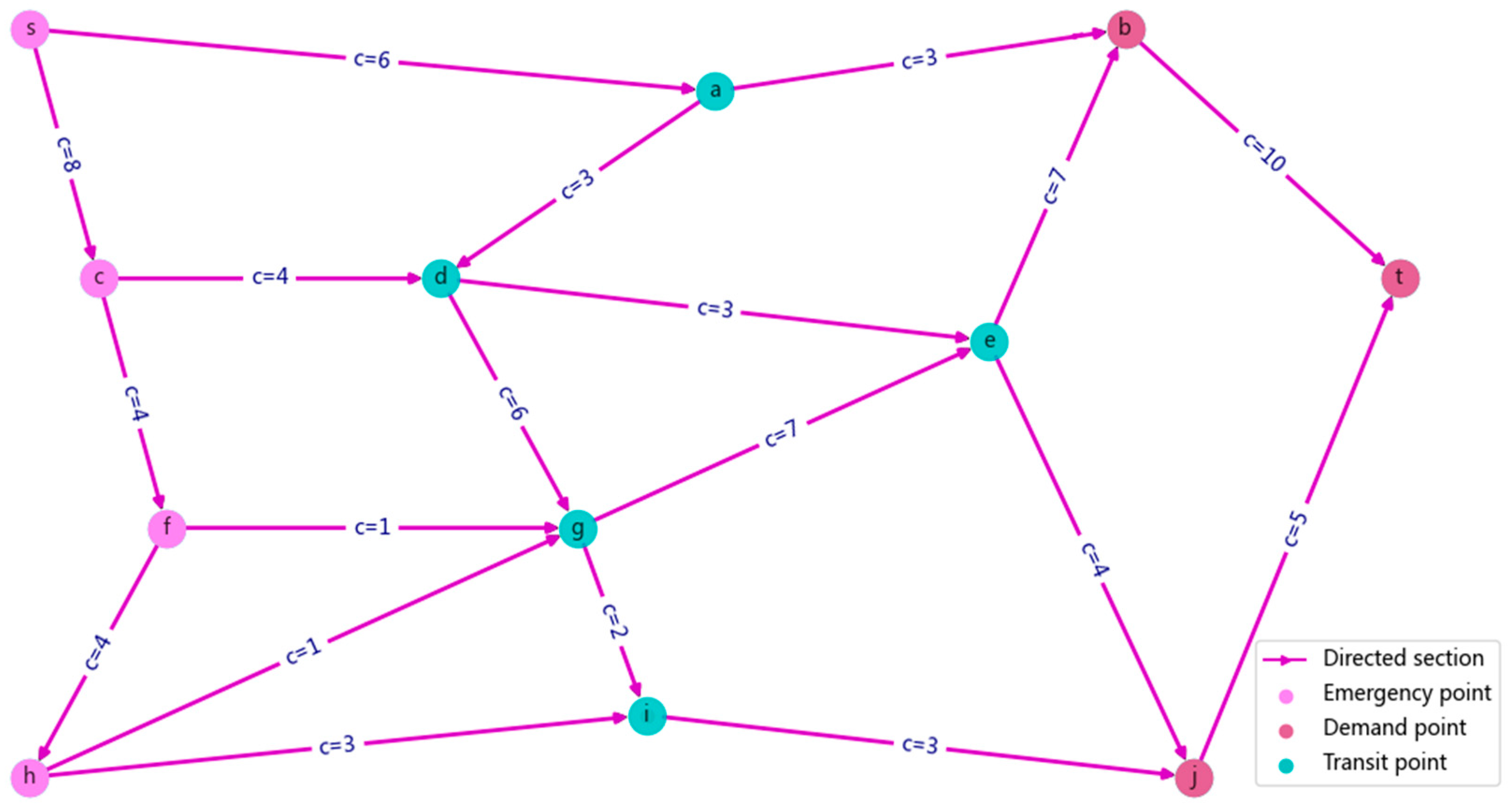
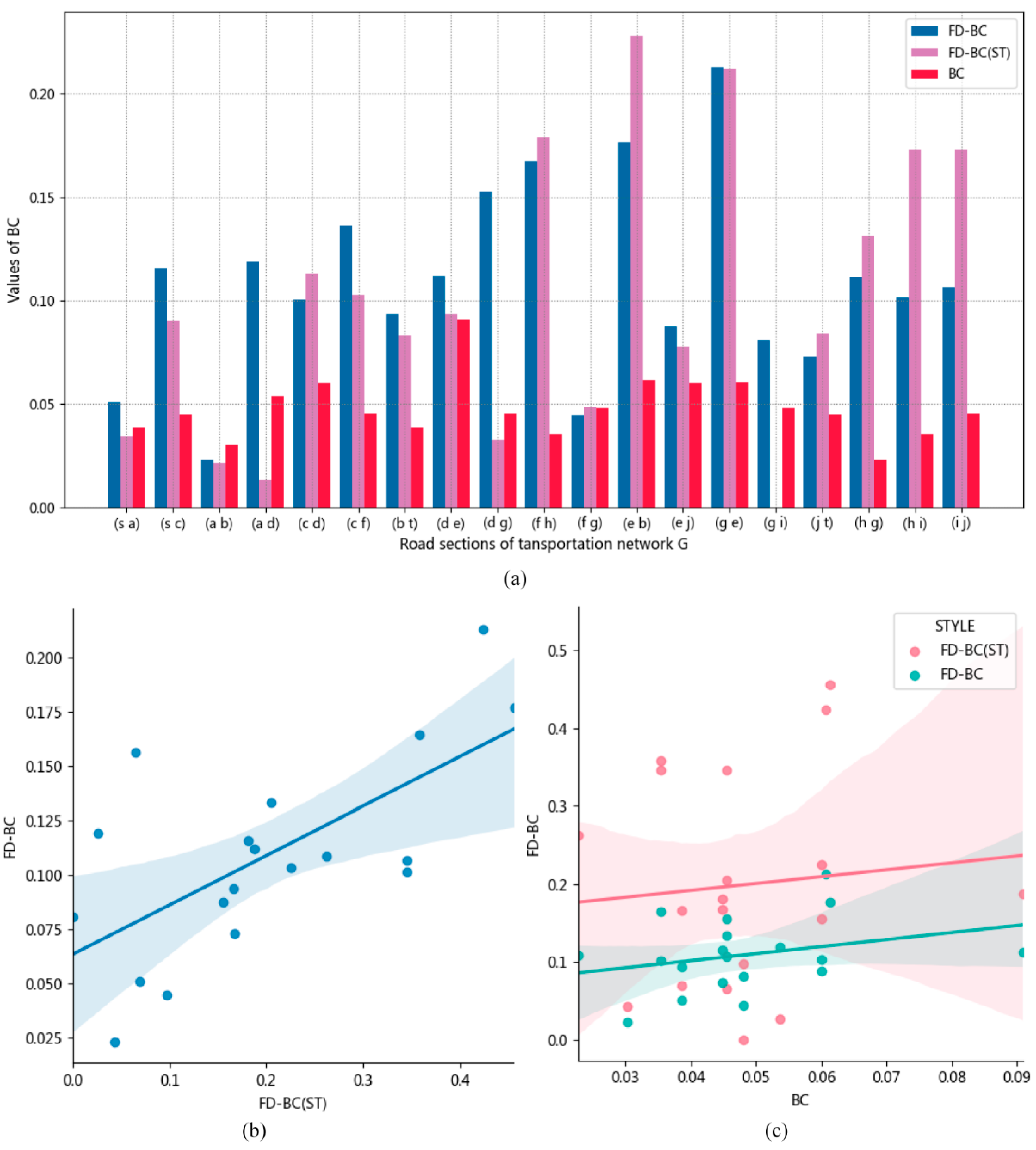
3.3.2. Flow Distributed Betweenness Centrality

The evaluation indicators based on the complex network topology structure include betweenness centrality (BC), efficiency of a network [48], degree and degree distribution [49,50], clustering coefficient [51], maximum connected subgraph [52], connectivity [53], etc. These indicators mainly evaluate the importance of network components (nodes, sections, etc.) from the perspective of complex network geometry and topology, with particular emphasis on the adjacency status and the spatial distance between elements. The evaluation index based on network operation performance mainly considers the role played by network components in the actual operation of complex networks and focuses on the analysis of traffic distribution and operation efficiency on complex network elements, such as flow intensity [54], flow efficiency [55,56], accessibility [57,58], etc.
The existing complex network evaluation indicators do not consider the limitation of transportation network capacity and the distribution of transport volume on the transportation network. They are only determined by the geometric topology and the demands of demand points. In addition, the emergency location model not only needs to consider the uncertainty of the transport capacity but also needs to account for the uncertainty of emergency point selection and transportation route matching. Therefore, in this paper, we proposed the concept of flow distributed betweenness centrality (FD-BC), and its calculation formula is as follows:
C F B ( i , j ) = s V t V f ( i , j ) ( s , t ) / f ( s , t ) N ( N 1 ) / a ,   ( i , j ) A , s t
Parameter a is the adjustment coefficient: a = 1 when the transportation network is a directed network, while a = 2 when the transportation network is an undirected network. N represents the number of edges in the network. FD-BC represents the expected value of the ratio of transport volume carried by the target road section to transportation network capacity under all possible combinations of the origin and destination points. The higher the value of FD-BC, the more crucial the road section is within the transportation network. The comparison between FD-BC and the existing complex network indicators is shown in Table 1.
In the location model, the origin points correspond to the emergency point set S , while the destination points correspond to the demand point set T , and S , T V . In other words, the scope of the sets to which the origin and the destination points belong in the location model is reduced. If Formula (14) is continuously applied under the background of an emergency, it will not only make the calculation result deviate from the actual situation but will also increase the time complexity of the calculations ( O ( | V | 2 ) > O ( | S | | T | ) ). Therefore, Formula (14) is improved, and the improved Formula (15) and its extended Formula (16) are as follows:
C F B S T ( i , j ) = s S t T f ( i , j ) ( s , t ) / f ( s , t ) | S | | T | ,   ( i , j ) A
S ( i , j ) ε ( u , v ) = max { C F B S T ( i , j | ( u , v ) , ε ) C F B S T ( i , j ) , 0 }
In order to distinguish from C F B ( i , j ) (FD-BC) in Formula (14), C F B S T ( i , j ) in Formula (15) is expressed as FD-BC (ST). In Formula (16), indicator S ( i , j ) ε ( u , v ) represents the maximum variation (non-negative) of FD-BC (ST) of road section ( i , j ) when the perturbation ratio of road section ( u , v ) is ε . Consequently, θ ( u , v ) S ( i , j ) ε ( u , v ) represents the expected ratio of the increase in transport volume in road section ( i , j ) when the uncertain value of the road section ( u , v ) is θ ( u , v ) , and the perturbation ratio is ε .
To express the increased transport volume on section ( i , j ) , Formula (17) is introduced:
f G a v e = s t f ( s , t ) / | S | | T | ,   s S , t T
Value f G a v e represents the expected maximum transport capacity of the transportation network G under all possible combinations of the emergency and demand points. Therefore, θ ( u , v ) S ( i , j ) ε ( u , v ) f G a v e represents the expected value of the increased transport volume carried by road section ( i , j ) when the uncertain value of road section ( u , v ) is θ ( u , v ) , and the perturbation ratio is ε .

3.3.3. Transport Capacity Effect Coefficient

According to Assumption (3), these unexpected increases in transport volume will cause secondary losses of transport capacity on certain road sections, known as indirect loss of transport capacity. To find the relationship between the unexpected increase in the transport volume of the road section and its corresponding indirect loss of transport capacity, we considered that the transport capacity of the road section exhibited a negative correlation with the unexpected increase in transport volume of the section. Therefore, referring to the model structure of the Smoch function applied in Detroit planning and the Overgaard impedance function [59], we constructed a function in exponential form that reflects the correlative relationship between the indirect loss of the transport capacity and the unexpected increase in the transport volume of the road section. The formula is as follows:
c ( i , j ) ε ( θ ( u , v ) ) = c ( i , j ) α β ( θ ( u , v ) S ( i , j ) ε ( u , v ) f G a v e / c ( i , j ) ) , ( i , j ) , ( u , v ) A
where c ( i , j ) ε ( θ ( u , v ) ) represents the transport capacity of road section ( i , j ) , given that the uncertainty value of road section ( u , v ) is θ ( u , v ) and the perturbation ratio is ε . In this way, a correlation relationship between the indirect loss of transport capacity on road section ( i , j ) and the direct loss of transport capacity on road section ( u , v ) within the transportation network is established under emergency circumstances. From Formula (18), we defined the transport capacity effect coefficient (TC-EC) of road section ( u , v ) on road section ( i , j ) , which is expressed as follows:
ρ ( i , j ) ε ( θ ( u , v ) ) = α β ( θ ( u , v ) S ( i , j ) ε ( u , v ) f G a v e / c ( i , j ) ) , ( i , j ) , ( u , v ) A
where ρ ( i , j ) ( θ ( u , v ) ) represents the retention proportion of transport capacity of section ( i , j ) , given that the uncertainty value of road section ( u , v ) is θ ( u , v ) and the perturbation ratio is ε . It should be noted that, generally, the TC-EC between road sections is not symmetrical, that is, ρ ( i , j ) ( θ ( u , v ) ) ρ ( u , v ) ( θ ( i , j ) ) .

3.3.4. Robust Location Model with Ellipsoidal Uncertainty Set Construction

It is necessary to consider expanding from the correlation between a single road section and the target road section to the correlation between all road sections of the transportation network and the target road section. Therefore, the transport capacity of the target road section ( i , j ) was firstly changed to ( c ( i , j ) θ ( i , j ) ε c ( i , j ) ) due to a direct loss resulting from the impact of emergencies, with ε c ( i , j ) being the maximum direct loss of the transport capacity of road section ( i , j ) . In addition, the transport capacity of road section ( i , j ) may be subject to indirect losses caused by all the relevant road sections. After comprehensively considering both the direct loss and indirect losses of the transport capacity of road section ( i , j ) , the transport capacity of road section ( i , j ) under the emergency state was denoted as c ˜ ( i , j ) , and the corresponding calculation formula is as follows:
c ˜ ( i , j ) = ( c ( i , j ) θ ( i , j ) ε c ( i , j ) ) ( u , v ) A ρ ( i , j ) ε ( θ ( u , v ) ) , ( i , j ) A
To facilitate the creation of robust counterparts of the location model, the existing Formula (20) was further modified and rearranged to obtain the following improved version:
c ˜ ( i , j ) = c ( i , j ) α β θ ( i , j ) ( log a ( 1 / ( 1 θ ( i , j ) ε ) ) / β θ ( i , j ) ) × α β ( u , v ) A ( θ ( u , v ) S ( i , j ) ε ( u , v ) f G a v e / c ( i , j ) ) , ( i , j ) A
We can observe that Formula (21) does not meet the mathematical requirements necessary for the direct application of robust optimization. To derive a robust counterpart of Formula (21) and ensure the stability of constraint condition (4), Formula (21) needs to be scaled appropriately: Let f ( θ ( i , j ) ) = log α ( 1 / ( 1 θ ( i , j ) ε ) ) / β θ ( i , j ) , when θ ( i , j ) , ε [ 0 , 1 ] , deriving f ( θ ( i , j ) ) with respect to θ ( i , j ) results in f ( θ ( i , j ) ) 0 , which indicates that f ( θ ( i , j ) ) is a monotonous non-decreasing function, and the maximum value of f ( θ ( i , j ) ) can be denoted as f ( 1 ) = β 1 log α ( 1 / ( c ( i , j ) ε ) ) . After replacing f ( θ ( i , j ) ) with f ( 1 ) in Formula (21) to complete the scaling process, the resulting modified formula is defined as follows:
c ( i , j ) s c a l i n g = c ( i , j ) α β θ ( i , j ) β 1 log α ( 1 / ( 1 ε ) ) × α β ( u , v ) A ( θ ( u , v ) S ( i , j ) ε ( u , v ) f G a v e / c ( i , j ) ) , ( i , j ) A
For f ( 1 ) f ( θ ( i , j ) ) , the transport capacity of road section ( i , j ) satisfies the relationship c ( i , j ) s c a l i n g c ˜ ( i , j ) c ( i , j ) , and constraint condition (4) becomes more conservative to ensure the stability of the model. At the same time, Formula (22) also has a mathematical form for transforming into the robust counterpart. Therefore, the ellipsoidal uncertainty set [60] was applied to describe the uncertainty values of the transportation network capacity, and the ellipsoidal uncertainty set is as follows:
θ ( i , j ) U e l l i p s o i d = { θ ( i , j ) : ( i , j ) A θ ( i , j ) 2 Ω 2 }
The parameter Ω represents the uncertainty level of the ellipsoidal uncertainty set. The larger the uncertainty level, Ω , is, the smaller the feasible space of the uncertainty set U e l l i p s o i d is, the stricter the constraints are, and the more conservative the robust model is. When the uncertain values of the transport capacity satisfy Formula (23), according to the robust optimization theory proposed by Ben-Tal, A., and Nemirovski, A. [31], the maximum value of part of the polynomial in the exponent on the right side of Formula (22) can be derived as:
θ ( i , j ) β 1 log a ( 1 / ( 1 ε ) ) + ( u , v ) A θ ( u , v ) S ( i , j ) ε ( u , v ) f G a v e / c ( i , j ) Ω ( β 1 log a ( 1 / ( 1 ε ) ) ) 2 + ( u , v ) A ( S ( i , j ) ε ( u , v ) f G a v e / c ( i , j ) ) 2 , ( i , j ) A
Replacing it in Formula (22) yielded the robust counterpart, which is defined as follows:
c ( i , j ) e l l i p s o i d = c ( i , j ) α β Ω ( β 1 log α ( 1 1 ε ) ) 2 + ( u , v ) A ( S ( i , j ) ε ( u , v ) f G a v e c ( i , j ) ) 2 , ( i , j ) A
To complete the transformation from the deterministic location model to the robust location model with the ellipsoidal uncertainty set, the initial transport capacity, c ( i , j ) , in the deterministic model was replaced with the robust optimized transport capacity, c ( i , j ) e l l i p s o i d ; meanwhile, as transport capacity decreases, transport time increases, and transport costs will rise. Consequently, the transport cost, e ( i , j ) , was replaced with the robust optimized transport cost, e ( i , j ) e l l i p s o i d . The formula is as follows:
e ( i , j ) e l l i p s o i d = e ( i , j ) c ( i , j ) / c ( i , j ) e l l i p s o i d , ( i , j ) A
Then, the objective function (2), objective function (3), and constraint (4) were transformed, as follows:
min f 2 = ( i , j ) A ω ( i , j ) ( s S t T f ( i , j ) ( s , t ) x s t c ( i , j ) e l l i p s o i d + σ ( i , j ) ) / c ( i , j ) e l l i p s o i d
min f 3 = s S k K ( p k y s k + d s h k ) + ( i , j ) A s S t T x s t e ( i , j ) e l l i p s o i d l ( i , j ) d t f ( i , j ) ( s , t ) f max ( s , t )
0 f ( i , j ) ( s , t ) + σ ( i , j ) c ( i , j ) e l l i p s o i d ,   ( i , j ) A , s S , t T
The other objective functions and constraints remained the same as those in the deterministic model, resulting in a robust location selection model with an ellipsoidal uncertainty set considering the correlation and uncertainty of transportation network capacity. The conservative degree can be adjusted by varying the value of the uncertainty level, Ω . When Ω = 0 , it was obtained that c ( i , j ) e l l i p s o i d = c ( i , j ) , which means that the robust model reduced to the nominal model.

4. Solution Procedure

4.1. Multi-Criteria Processing

In the location model of this paper, the dimensions of the three objectives are inconsistent, making the simple linear weighted method inadequate for accurately reflecting the differences in measurement units and orders of magnitude across objectives. Furthermore, different decision-makers exhibit varying risk preferences. Therefore, we used both the epsilon constraint method and the ideal point-based objective perturbation minimization method to provide a range of decision-support solutions considering different preferences and possible situations.

4.1.1. Epsilon Constraint Method

The epsilon constraint method [60,61] is a multi-objective processing method that transforms one of the objective functions into a constraint condition to limit the value range of the objective function. The location model presented in this paper first guarantees the lower minimum transport capacity of the emergency transportation network for each demand point and its corresponding emergency point then converts the objective function, f 1 , into a constraint condition, f 1 δ , through the epsilon constraint method. The threshold, δ , represents the lower limit of transport capacity, which depends on the value range of the objective function and the degree of risk preference of the decision-makers.

4.1.2. Ideal Point-Based Objective Perturbation Minimization Method

Under the premise of not considering other objectives, the optimal values’ combination obtained by considering only a single objective function is referred to as the ideal point of the multi-objective optimization model [62], representing an ideal state. After transforming the objective function, f 1 , into constraint conditions through the epsilon constraint method, assuming that ( f 2 * , f 3 * ) is an ideal point of the model, for any objective function f i , Δ i is defined as the perturbation value of the objective function, f i :
Δ i = | f i f i * | / f i * ,   i = 2.3
Let ω i represent the degree of preference that a decision-maker holds for various decision objectives; then, the multi-objective model is transformed into a target perturbation minimization model based on ideal points:
min max ω i Δ i ,   i = 2 , 3

4.2. Multi-SEGA

Under the condition of uncertain transport capacity, the robust optimization model for emergency location incorporates product terms of decision variables and uncertainty constraints, making the model solve a complex nonlinear optimization problem. To effectively solve the problem of model solving, we applied the multi-strength elitist genetic algorithm (multi-SEGA) [63,64], which uses a parallel distribution of sub-populations to complete the evolutionary process.

4.2.1. Fitness Function

The fitness function is expressed in Formula (32):
f i t = M | c v j | min max ω i Δ i
When an individual satisfies constraint c v j in the location model, c v j = 0 ; otherwise, its actual value is calculated. The parameter M is a sufficiently small negative number, and the meaning of min max ω i Δ i is the same as that described in Formula (31).

4.2.2. Individual Encoding and Population Initialization

Decision vectors Y s k and X s t correspond to decision variables y s k and x s t , respectively. | S | , | T | , and | K | represent the number of emergency points, demand points, and emergency material reserve types, respectively. The individual length of Y s k , determined by the number of emergency points and the types of emergency material reserves, is | S | × ( | K | + 1 ) . Meanwhile, the individual length of X s t , determined by the number of emergency and demand points, is | S | × | T | . In addition, | S | × ( | T | + | K | + 1 ) represents the length of the individual corresponding to each solution. We adopted binary coding. Moreover, the initial population was divided into specific subpopulations based on the needs of the model solution.

4.2.3. Genetic Operator

(1)
Selection operations
The multi-SEGA algorithm consists of a two-stage selection process. The first stage uses the tournament selection operator. In the second stage, the sorting operator is applied to each subpopulation separately.
(2)
Crossover operation
In the crossover operation stage, a two-point crossover operator is used to set a different crossover rate for each subpopulation.
(3)
Mutation operation
The mutation operation employs the mutation mechanism from the breeder genetic algorithm (BGA) [64], and this BGA operator utilizes the shrinkage rate and gradient division to control the mutation distance.

4.2.4. Population Migration

After each subpopulation has evolved independently for a certain number of generations, the information exchange between the subpopulations is completed through the population migration operation. The corresponding migration probabilities are set for different subpopulations. The migration structure is set as circular, meaning that it is transferred increasingly according to the subscript of the subpopulation. Moreover, the method of selecting emigrating individuals is based on choosing the best ones, and random substitution is used to replace the migrating individuals.

4.2.5. Algorithm Process

After completing the above parameter settings, the flowchart of the multi-SEGA is shown in Figure 2.

5. Case Analysis Example

5.1. Background Description

To verify the validity of the model, a small-scale emergency transportation network topology graph, G , was designed to simulate the process of emergency location and emergency materials’ distribution during the preparatory stages of an emergency. The transportation network topology graph, G , consists of a node set, N , which includes three subsets of emergency point set, S = { s , c , f , h } , demand point set, T = { b , t , j } , and transit point set, M = { a , d , g , i , e } , with a total of twelve transportation network nodes. A certain number of emergency points in the emergency point set S was selected to establish a corresponding type of emergency material reserve, and a certain amount of emergency rescue materials was reserved to meet the needs of the demand points under emergencies. The nodes in the transit point set M = { a , d , g , i , e } do not account for emergency reserves or have any demand for emergency materials and only have the function of emergency materials’ transfer. Adjacent nodes are connected by directed road sections (for example, road section ( a , b ) represents a directed road section from node a to node b ). Figure 3 shows the location distribution and topological relationship of nodes and sections of the emergency transportation network and the initial transport capacity of all road sections.
The road section ( i , j ) of the emergency transportation network G consists of three attributes, including the initial transport capacity, c ( i , j ) , the transport distance, l ( i , j ) , and the flow distribution betweenness centrality, C F B S T ( i , j ) . The initial transport capacity, c ( i , j ) , is the transport capacity of the road section ( i , j ) without being affected by emergencies. The transport distance, l ( i , j ) , is the length of the road section ( i , j ) , and the initial cost, e ( i , j ) , for transporting one cubic meter of cargo per 1000 m was set to 1000 Yuan. The values of the three attributes of all the road sections of the transportation network G are shown in Table 2. The emergency material reserve type is defined as K = { k 1 , k 2 , k 3 , k 4 } , which includes four types of options. Furthermore, each type of emergency material reserve has a corresponding fixed construction cost, p k , a unit emergency material storage cost, h k , and a maximum emergency material storage capacity, u k , and their corresponding values are shown in Table 3. It was assumed that the emergency materials required by the emergency demand points mainly include four types: water, food, medical supplies, and emergency tents. The required quantities of these materials were converted into volume (cubic meters) according to a specific ratio, as shown in Table 4.
To compare the differences between BC (betweenness centrality), FD-BC (a modified version of BC), and FD-BC (ST) (a special type of FD-BC for the location model), the transportation network G , which is illustrated in Figure 4, was used as a simulation example. Figure 4a presents the values of BC, FD-BC, and FD-BC (ST), while Figure 4b,c display their correlation coefficients.

5.2. Calculation Results and Analysis

5.2.1. Parameter Setting

Python3.8 was used to write the operation program of the robust location model, and the multi-strength elitist genetic algorithm (multi-SEGA) was applied to solve the model. In addition, an Intel (R) Core (TM) i5-7200U computer with 2.60 GHz and 8.00 GB RAM was used to run the calculations. The adopted encoding form and iteration logic are shown in Figure 2, and the parameters of the multi-SEGA were set as follows: the number of subpopulations was N g r o u p = 4 , the size of the subpopulations was N p i = 1000 , the minimum and maximum values of the crossover operation rates in the subpopulations were p c min = 0.7 and p c max = 1.0 , respectively, the shrinkage operator ratio was M u t S h r i n k = 0.5 , the gradient division grad was G r a d i e n t = 10 , the independent evolution algebra number was g M i g = 10 , and the rate of exchanging individuals between subpopulations was p M i g = 0.2 . By referencing relevant literature on the impedance function [61] and conducting a comparative analysis of model operations, the possible value ranges of the undetermined parameters, α and β , were analyzed. In this paper, the values of the parameters were set as α = 2 and β = 4 .

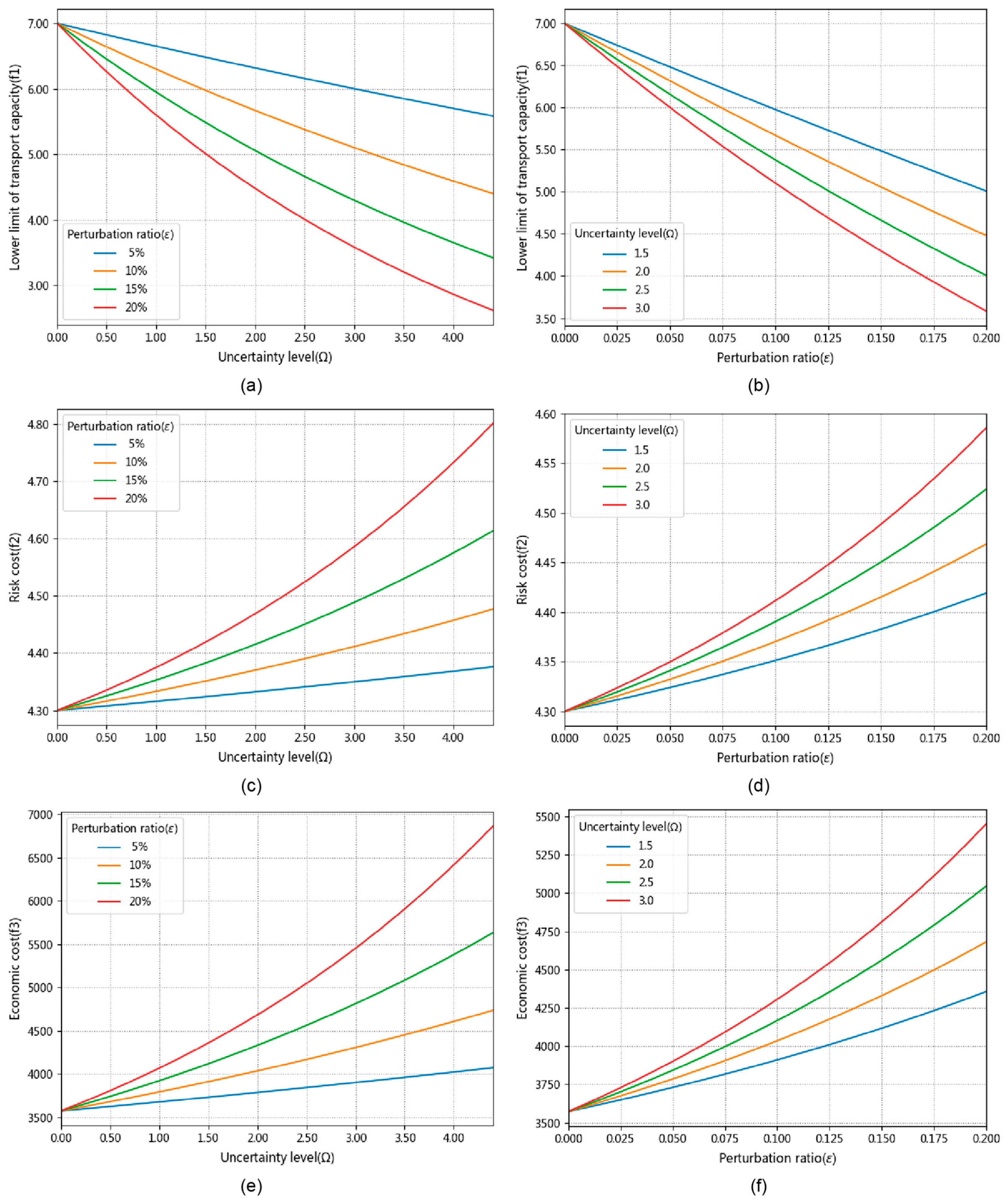
5.2.2. Perturbation Ratio and Uncertainty Level Analysis

Assuming all road sections of the transportation network exhibited the same perturbation ratio, ε , the higher the perturbation ratio ε , the greater the range of the uncertainty set in transport capacity within the transportation network. The robust model with an ellipsoidal uncertainty set can adjust the conservative degree of the model through uncertainty level Ω . When Ω = 0 , the transport capacity of the transportation network was a definite initial value, and the robust model was equivalent to the deterministic model. When Ω 0 , the robust model tended to be more stable as the value of the uncertainty level Ω increased.
Under different combinations of the perturbation ratio, ε , and the uncertainty level, Ω , the optimal values of the objective functions in the robust model showed distinct trends, ultimately influencing the decision-making results. In order to analyze the variation in the optimal values of the objective functions in the robust model to the uncertainty level, Ω , and perturbation ratio, ε , the optimal values of the three objective functions under different uncertainty levels, Ω , were calculated, respectively, for four states of the perturbation ratios ( ε = 0.05 , ε = 0.10 , ε = 0.15 , and ε = 0.20 ). Similarly, the optimal values of the three objective functions under different perturbation ratios, ε , were calculated, respectively, for four states of the uncertainty levels ( Ω = 1.5 , Ω = 2.0 , Ω = 2.5 , and Ω = 3.0 ) [35,37]. The results are shown in Figure 5.
As observed from Figure 5a,b, the curves depicting the lower limit of transport capacity exhibited a gradual variation with changes in the perturbation ratio, ε , and uncertainty level, Ω , indicating that the lower limit of transport capacity was not highly sensitive to the perturbation ratio, ε , or uncertainty level, Ω . This demonstrated that the robust model in this paper could guarantee the emergency transport capacity between the emergency points and the demand points while simultaneously ensuring robustness.
In contrast, as observed from Figure 5c–f, the curves depicting risk cost and economic cost became more curved with the increase in the perturbation ratio, ε , and uncertainty level, Ω , indicating that both the risk cost and economic cost were sensitive to perturbation ratio, ε , and uncertainty level, Ω . The robust model in this paper needs to sacrifice higher risk cost and economic cost to maintain robustness as the perturbation ratio, ε , and uncertainty level, Ω , increase. It can also be inferred that as the perturbation ratio, ε , and uncertainty level, Ω , increased, the risk cost and economic cost per unit of the lower limit of transport capacity increased accordingly.
Therefore, it is crucial to achieve a reasonable combination of the perturbation ratio, ε , and the uncertainty level, Ω , which can effectively balance both model stability and economy. The perturbation ratio, ε , and the uncertainty level, Ω , are generally selected based on available information or the preferences of decision-makers. For the uncertainty level, Ω , aside from the aforementioned methods, on the premise that the perturbation ratio, ε , is determined, we can compare optimal values of the objective functions in the robust model with an ellipsoidal uncertainty set to those of both the deterministic model and the robust model with a boxed uncertainty set (considering the indirect loss of transport capacity as well). This comparison ensures that the degree of conservatism of the robust model with ellipsoidal uncertainty falls between the degrees of conservatism of the deterministic model and the robust model with a boxed uncertainty set.
In this article, we assumed that the perturbation ratio ε = 0.1 , and the comparison process of the optimal values of the three models is shown in Figure 6.
As shown in Figure 6, at a disturbance ratio of ε = 0.1 , when the uncertainty level Ω = 0 , the robust model with the ellipsoidal uncertainty set coincided with the nominal model and tended to become more conservative as the uncertainty level increased. When the uncertainty level, Ω , was within the interval [2, 2.5], the degree of conservatism approached that of the robust model with a box uncertainty set. When the uncertainty level, Ω , was greater than the pink dotted line, the model was no longer meaningful. After the above analysis, we assumed that the uncertainty level Ω = 1.5 .

5.2.3. Model Solving

After determining the perturbation ratio, ε , and the uncertainty level, Ω , the robust model with an ellipsoidal uncertainty set should be solved, and the corresponding decision should be given. The solution steps are as follows:
(1)
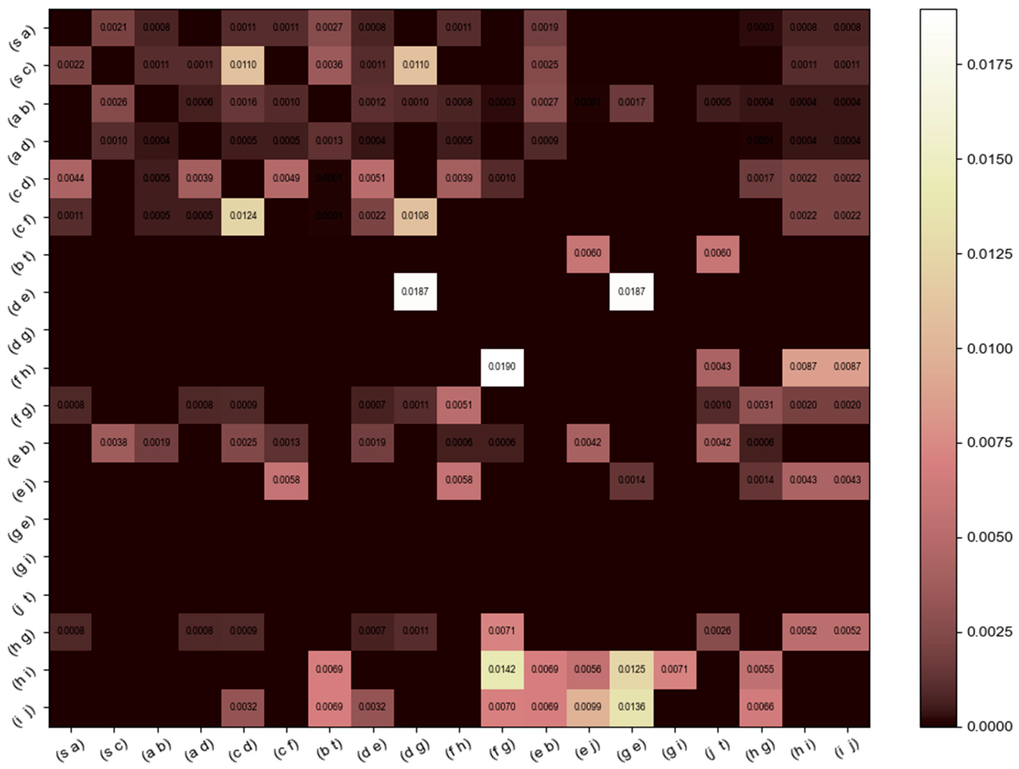
Calculate the matrix of the maximum variation (non-negative) of the FD-BC (ST) indicator of the emergency transportation network G (perturbation ratio ε = 10 % ), as shown in Figure 7. Then, derive the transport capacity of the transportation network G considering the correlation of transport capacity under the influence of emergency.
(2)
Update the transport cost of emergency materials in the emergency state. Furthermore, determine the optimal values of each objective function of the robust model without considering the constraints from other objective functions.
(3)
Use the epsilon constraint method to transform the original objective function (1) into a new constraint, thereby ensuring the maintenance of a minimum transport capacity between the demand points and their corresponding emergency points in the emergency transportation network G . At the same time, it will also affect the optimal value of function (2) and function (3), as shown in Figure 8.
(4)
By adjusting the combination of weights ω 2 and ω 3 of the objective functions (2) and (3), generating multiple scenarios to reflect different decision-makers’ preferences, the ideal point-based target perturbation minimization method is applied for multi-objective processing in each scenario.
(5)
Apply two algorithms, multi-SEGA and SGA, to solve the robust model. Repeat this process 20 times to record the results and select the results with the best effect for comparison. The iterative process and calculation results are shown in Figure 9 and Table 5, respectively.
In Figure 7, each value in the matrix represents the maximum variation (non-negative) of the FD-BC (ST) indicator of each corresponding road section along the x-axis when the perturbation ratio, ε , of the corresponding road section along the y-axis was 10%; the larger the value, the greater the transport capacity effect coefficient (TC-EC) of the road section along the y-axis.
From Figure 8a, we observed that the risk cost ( f 2 ) of all three types of models increased as the lower limit of transport capacity increased. This is because some sections with smaller transport capacities were discarded, which intensified the tendency for the transport volume between different emergency points and demand points to overlap in some sections. From Figure 8b, we observed that the economic cost ( f 3 ) increased with the rise in the lower limit of transport capacity. The reason for this is that some transport routes with shorter transport distances were discarded, as they did not meet the requirements of transport capacity, which also affected the selection of the emergency material reserve types, thus increasing the economic cost.
Figure 9 shows the iterative process of applying the multi-SEGA and the standard genetic algorithm (SGA) to the robust model with the ellipsoidal uncertainty set under a specific model parameter value ( f 1 4 , ε 2 = 0.5 , and ε 3 = 0.5 ). The yellow line tracks the best objective value over iterations, while the blue line tracks the average. The multi-SEGA achieved a steady state after an average of 38 generations, while the SGA required approximately 130 generations. Moreover, the multi-SEGA has certain advantages in efficiency and stability compared with the SGA. Due to the establishment of four parallel subpopulations in the multi-SEGA, and each subpopulation had different crossover and mutation ratios. Therefore, the parallel solution process can balance the search speed and accuracy. However, the augmented initial population size of the multi-SEGA requires more computational space.
Table 5 presents the optimal location results of the robust location model with the ellipsoidal uncertainty set based on the specific combination of corresponding conditions. The left-hand side of Table 5 indicates the specified range for the lower limit of transport capacity ( f 1 ). The top of Table 5 displays various weight combinations for the objective functions, balancing risk cost ( f 2 ) and economic cost ( f 3 ). As a demonstration, the result corresponding to f 1 3 , ε 2 = 0.5 , and ε 3 = 0.5 in Table 5 was ( h t , h j , c b , c k 1 , h k 3 ), which means that the decision-maker limited the lower limit of transport capacity, f 1 3 , and had an equal preference for f 2 and f 3 . The optimal result obtained was as follows: emergency point c supplying to demand point b , point h supplying to demand point j and point t , and building a k 1 -type emergency material reserve at point c and a k 3 -type reserve at point h .
Due to space limitations, we only presented the calculation results of the five weight combinations of the objective functions under the conditions of perturbation ratio ε = 0.1 and uncertainty level Ω = 1.5 . Relevant departments can simulate numerous potential scenarios ahead of time and record the simulation calculation results so that decision-makers can quickly make decisions according to the actual situation and personal risk preference and refer to the results in the record table.

6. Conclusions

Emergencies have significant impacts on human life and civil infrastructure. During emergencies, a comprehensive and robust emergency support system is the crucial safeguard to control the deterioration of the situation and minimize casualties and economic losses. The construction of such an emergency support system should not only cater to the demand for emergency materials but also address the challenges posed by the uncertainty of transportation networks. Therefore, accounting for the uncertainty in transport capacity, we proposed a robust location model. In this model, the concepts of flow distribution betweenness centrality (FD-BC) and the transport capacity effect coefficient (TC-EC) were introduced, and the importance of each road section in the transportation network was measured through FD-BC, while the correlation between transport capacities of road sections was measured through TC-EC. Furthermore, an ellipsoidal uncertainty set was introduced to describe the uncertainty in transportation network capacity. In addition, a robust emergency location model based on the ellipsoidal uncertainty set was constructed. This robust model considers multi-criteria of the lower limit of transport capacity, risk cost, and economic cost. Finally, by designing an uncertain scenario example, the influence of the perturbation ratio, ε , and the uncertainty level, Ω , on the objective function was analyzed, and the parameters of the robust model with an ellipsoidal uncertainty set were determined by comparing it with the excessively optimistic deterministic model and the conservative robust model with a box uncertainty set.
Furthermore, there were some implications, as follow:
(1)
Compared with FD-BC, the indicator FD-BC (ST) could more accurately reflect the importance of a specific section in the emergency transportation network during the transportation process of emergency materials, significantly reducing the complexity of calculations and saving decision-making time.
(2)
The robust model with an ellipsoidal uncertainty set demonstrated that the assumption that the transport capacity of the road network is susceptible to damage from a sudden increase in traffic volume was closer to reality. Furthermore, the uncertainty of all road sections can be expressed by an uncertainty level, Ω , through the robust equivalence form.
However, due to the lack of information about the uncertain distribution of transportation capacity and the mathematical characteristics of the ellipsoidal robust model, the model constructed here tended to be overly conservative, and its practical application effect needs to be enhanced. In the future, machine learning can be considered to address this mathematical limitation. At the same time, this paper simulated a small transportation network. When the model expanded to an expanded transportation network, the running speed did not scale appropriately with the desired actual effect. Next, we will find a way to simplify the processing of large transportation networks, optimize the speed of the simulation, and enhance the practical applicability of the model.

Author Contributions

Conceptualization, B.J.; methodology, B.J.; software, B.J.; validation, Y.S.; formal analysis, B.J.; investigation, B.J.; resources, Y.S.; data curation, B.J.; writing—original draft preparation, B.J.; writing—review and editing, Y.S.; visualization, B.J.; supervision, Y.S.; project administration, Y.S.; funding acquisition, Y.S. All authors have read and agreed to the published version of the manuscript.

Funding

This research was supported by the National Natural Science Foundation of China (No. 71771061).

Data Availability Statement

Data are contained within the article.

Conflicts of Interest

The authors declare no conflicts of interest.

Abbreviations

V Set of transportation network nodes, indexed by nodes i , j V , and i j
A Set of transportation network sections. If nodes i and j are adjacent, then section ( i , j ) A
C Set of transport capacities of road sections
L Set of road section lengths in the transportation network
G Weighted emergency transportation network, G = ( V , A , C , L )
S Set of emergency points, emergency point s S
T Set of demand points, demand point t T
K Type of emergency material reserves, available reserve type k K
l ( i , j ) Transport length of road section ( i , j ) , l ( i , j ) L
c ( i , j ) Transport capacity of road section ( i , j ) , c ( i , j ) C
p k Fixed construction cost of establishing type k emergency material reserve
h k Storage cost per unit volume of emergency material reserve of type k
u k Upper inventory limit of type k emergency material reserve
d s Expected emergency material reserved at the emergency point s
d t Expected emergency material demand at the demand point t
e ( i , j ) Initial transport cost of emergency materials of road section ( i , j )
θ ( i , j ) Uncertain value of the transport capacity of road section ( i , j ) , and θ ( i , j ) [ 0 , 1 ]
σ ( i , j ) Traffic volume of non-emergency materials in section ( i , j )
ε Perturbation ratio, which determines the range of the uncertain set of transport capacity, ε [ 0 , 1 ]
n Number of nodes selected from emergency point set S to establish emergency material reserves, n | S |
ω ( i , j ) Penalty factor, which indicates that the volume of materials carried by road section ( i , j ) exceeds its transport capacity, is a constant greater than zero; otherwise, it is zero
f ( s , t ) Volume of emergency materials that can be transported from emergency point s to demand point t on the transportation network
f ( i , j ) ( s , t ) Volume of emergency materials transported from emergency point s to demand point t , carried by road section ( i , j )
x s t Binary location decision variable x s t { 0 , 1 } ; when x s t is equal to 1, it means that the emergency point s provides emergency supplies to demand point t
y s k Binary location decision variable y s k { 0 , 1 } ; when y s k is equal to 1, it means that the type k emergency material reserve is established at the emergency point s
F Lower limit of transport capacity required between all the emergency points and the demand points

References

  1. St. Denis, L.A.; Short, K.C.; McConnell, K.; Cook, M.C.; Mietkiewicz, N.P.; Buckland, M.; Balch, J.K. All-hazards dataset mined from the US National Incident Management System 1999–2020. Sci. Data 2023, 10, 112. [Google Scholar] [CrossRef] [PubMed]
  2. Summers, J.K.; Lamper, A.; McMillion, C.; Harwell, L.C. Observed changes in the frequency, intensity, and spatial patterns of nine natural hazards in the United States from 2000 to 2019. Sustainability 2022, 14, 4158. [Google Scholar] [CrossRef] [PubMed]
  3. Petrova, E. Natural hazard impacts on transport infrastructure in Russia. Nat. Hazards Earth Syst. Sci. 2020, 20, 1969–1983. [Google Scholar] [CrossRef]
  4. Yu, Q.; Wang, Y.; Li, N. Extreme flood disasters: Comprehensive impact and assessment. Water 2022, 14, 1211. [Google Scholar] [CrossRef]
  5. Koks, E.E.; Rozenberg, J.; Zorn, C.; Tariverdi, M.; Vousdoukas, M.; Fraser, S.A.; Hall, J.W.; Hallegatte, S. A global multi-hazard risk analysis of road and Railway Infrastructure Assets. Nat. Commun. 2019, 10, 2677. [Google Scholar] [CrossRef] [PubMed]
  6. Wang, W.; Wu, S.; Wang, S.; Zhen, L.; Qu, X. Emergency facility location problems in Logistics: Status and Perspectives. Transp. Res. Part E Logist. Transp. Rev. 2021, 154, 102465. [Google Scholar] [CrossRef]
  7. Wang, S.L.; Sun, B.Q. Model of multi-period emergency material allocation for large-scale sudden natural disasters in humanitarian logistics: Efficiency, effectiveness and equity. Int. J. Disaster Risk Reduct. 2023, 85, 103530. [Google Scholar] [CrossRef]
  8. Hou, L.-X.; Mao, L.-X.; Liu, H.-C.; Zhang, L. Decades on emergency decision-making: A bibliometric analysis and literature review. Complex. Intell. Sys. 2021, 7, 2819–2832. [Google Scholar] [CrossRef] [PubMed]
  9. Jalil, S.A.; Javaid, S.; Muneeb, S.M. A decentralized multi-level decision making model for solid transportation problem with uncertainty. Int. J. Syst. Assur. Eng. Manag. 2018, 9, 1022–1033. [Google Scholar] [CrossRef]
  10. Qu, S.; Wang, L.; Ji, Y.; Zuo, L.; Wang, Z. The strategic weight manipulation model in uncertain environment: A robust risk optimization approach. Systems 2023, 11, 151. [Google Scholar] [CrossRef]
  11. Lu, M.; Shen, Z.M. A review of robust operations management under model uncertainty. Prod. Oper. Manag. 2021, 30, 1927–1943. [Google Scholar] [CrossRef]
  12. Bomze, I.M.; Gabl, M. Optimization under uncertainty and risk: Quadratic and Copositive approaches. Eur. J. Oper. Res. 2023, 310, 449–476. [Google Scholar] [CrossRef]
  13. Ma, Y.; Xu, W.; Qin, L.; Zhao, X. Site selection models in natural disaster shelters: A Review. Sustainability 2019, 11, 399. [Google Scholar] [CrossRef]
  14. Liu, Y.; Yuan, Y.; Shen, J.; Gao, W. Emergency response facility location in Transportation Networks: A literature review. J. Traffic Transp. Eng. Engl. Ed. 2021, 8, 153–169. [Google Scholar] [CrossRef]
  15. Church, R.L.; Drezner, Z. Review of Obnoxious Facilities Location Problems. Comput. Oper. Res. 2022, 138, 105468. [Google Scholar] [CrossRef]
  16. Geoffrion, A.M.; Powers, R.F. Twenty Years of strategic distribution system design: An evolutionary perspective. Interfaces 1995, 25, 105–127. [Google Scholar] [CrossRef]
  17. Usmani, R.S.; Hashem, I.A.; Pillai, T.R.; Saeed, A.; Abdullahi, A.M. Geographic Information System and big spatial data. Int. J. Enterp. Inf. Syst. 2020, 16, 101–145. [Google Scholar] [CrossRef]
  18. Wolf, G.W. Solving location-allocation problems with professional optimization software. Trans. GIS 2022, 26, 2741–2775. [Google Scholar] [CrossRef]
  19. Wang, Z.; Hao, S.; Yuan, L.; Hao, K. A three-stage stochastic model to improve resilience with lateral transshipment in multi-period emergency logistics. Systems 2024, 12, 73. [Google Scholar] [CrossRef]
  20. Chen, H.; Murray, A.T.; Jiang, R. Open-source approaches for location cover models: Capabilities and efficiency. J. Geogr. Syst. 2021, 23, 361–380. [Google Scholar] [CrossRef]
  21. Wang, Y.; Xu, Z. A multi-objective location decision making model for emergency shelters giving priority to subjective evaluation of residents. Int. J. Comput. Commun. 2022, 17, 4749. [Google Scholar] [CrossRef]
  22. Yu, W. Robust model for discrete competitive facility location problem with the uncertainty of customer behaviors. Optim. Lett. 2020, 14, 2107–2125. [Google Scholar] [CrossRef]
  23. Zhang, J.; Huang, J.; Wang, T.; Zhao, J. Dynamic optimization of emergency logistics for major epidemic considering demand urgency. Systems 2023, 11, 303. [Google Scholar] [CrossRef]
  24. Wang, Y.; Xu, Z. An emergency shelter location model based on the sense of security and the reliability level. J. Syst. Sci. Syst. Eng. 2023, 32, 100–127. [Google Scholar] [CrossRef]
  25. Peng, D.; Ye, C.; Wan, M. A multi-objective improved novel discrete particle swarm optimization for Emergency Resource Center Location Problem. Eng. Appl. Artif. Intel. 2022, 111, 104725. [Google Scholar] [CrossRef]
  26. Ahmadi-Javid, A.; Ramshe, N. Linear formulations and valid inequalities for a classic location problem with congestion: A robust optimization application. Optim. Lett. 2019, 14, 1265–1285. [Google Scholar] [CrossRef]
  27. Nayeri, S.; Tavakoli, M.; Tanhaeean, M.; Jolai, F. A robust fuzzy stochastic model for the Responsive-Resilient Inventory-location problem: Comparison of metaheuristic algorithms. Ann. Oper. Res. 2021, 315, 1895–1935. [Google Scholar] [CrossRef]
  28. Basciftci, B.; Ahmed, S.; Shen, S. Distributionally robust facility location problem under decision-dependent stochastic demand. Eur. J. Oper. Res. 2021, 292, 548–561. [Google Scholar] [CrossRef]
  29. Shi, J.; Zheng, X.; Jiao, B.; Wang, R. Multi-scenario cooperative evolutionary algorithm for the β-robust P-median problem with demand uncertainty. Appl. Sci. 2019, 9, 4174. [Google Scholar] [CrossRef]
  30. Li, X.; Zhang, T.; Wang, L.; Ma, H.; Zhao, X. A minimax regret model for the leader–follower facility location problem. Ann. Oper. Res. 2020, 12, 104–110. [Google Scholar] [CrossRef]
  31. Lai, Z.; Wang, Z.; Ge, D.; Chen, Y. A multi-objective robust optimization model for emergency logistics center location. Oper. Res. Manag. Sci. 2020, 29, 74–83. [Google Scholar] [CrossRef]
  32. Ardestani-Jaafari, A.; Delage, E. Linearized robust counterparts of two-stage robust optimization problems with applications in Operations Management. INFORMS J. Comput. 2021, 33, 1138–1161. [Google Scholar] [CrossRef]
  33. Xu, L.; Zhou, J. Robust optimization of multiple logistics nodes location problem with curved demands. In Proceedings of the 2020 4th International Conference on Management Engineering, Software Engineering and Service Sciences, Wuhan, China, 17 January 2020; pp. 245–249. [Google Scholar] [CrossRef]
  34. Sun, H.; Xiang, M.; Xue, Y. Robust Optimization for Emergency Location-Routing Problem with Uncertainty. J. Syst. Manag. 2019, 28, 1126–1133. [Google Scholar] [CrossRef]
  35. Wu, D.; Chen, F. The distributionally robust inventory strategy of the overconfident retailer under supply uncertainty. Systems 2023, 11, 333. [Google Scholar] [CrossRef]
  36. Chen, G.; Fu, J. Research on robust location for emergency medical mobile hospital under uncertain demand after disasters. Chin. J. Manag. Sci. 2021, 29, 213–222. [Google Scholar]
  37. Zhang, M.; Huang, T.; Guo, Z.; He, Z. Complex-network-based traffic network analysis and Dynamics: A comprehensive review. Physica A 2022, 607, 128063. [Google Scholar] [CrossRef]
  38. Cai, Q.; Alam, S.; Liu, J. On the robustness of complex systems with multipartitivity structures under node attacks. IEEE Trans. Control Netw. 2020, 7, 106–117. [Google Scholar] [CrossRef]
  39. Li, M.; Wang, H.; Wang, H. Resilience Assessment and Optimization for Urban Rail Transit Networks: A case study of Beijing subway network. IEEE Access 2019, 7, 71221–71234. [Google Scholar] [CrossRef]
  40. Yang, Y.; Liu, Y.; Zhou, M.; Li, F.; Sun, C. Robustness assessment of urban rail transit based on complex network theory: A case study of the Beijing subway. Saf. Sci. 2015, 79, 149–162. [Google Scholar] [CrossRef]
  41. Sun, R.; Zhu, G.; Liu, B.; Li, X.; Yang, Y.; Zhang, J. Vulnerability analysis of urban rail transit network considering Cascading Failure Evolution. J. Adv. Transp. 2022, 2022, 2069112. [Google Scholar] [CrossRef]
  42. Liu, J.; Yang, X.; Ren, S. Research on the impact of heavy rainfall flooding on urban traffic network based on road topology: A case study of Xi’an city, China. Land 2023, 12, 1355. [Google Scholar] [CrossRef]
  43. Li, J.; Yue, Q.; Huang, Z.; Xie, X.; Yang, Q. Vulnerability Analysis of UAV SWARM network with emergency tasks. Electronics 2024, 13, 2005. [Google Scholar] [CrossRef]
  44. Song, S.; Wang, S.-H.; Shi, M.-X.; Hu, S.-S.; Xu, D.-W. Multiple scenario simulation and optimization of an urban green infrastructure network based on complex network theory: A case study in Harbin city, China. Ecol. Process 2022, 11, 33. [Google Scholar] [CrossRef]
  45. Zheng, S.; Yang, H.; Hu, H.; Liu, C.; Shen, Y.; Zheng, C. Station placement for Sustainable Urban Metro Freight Systems using complex network theory. Sustainability 2024, 16, 4370. [Google Scholar] [CrossRef]
  46. Wu, P.; Li, Y.; Li, C. Invulnerability of the urban agglomeration integrated passenger transport network under emergency events. Int. J. Environ. Res. Public Health 2022, 20, 450. [Google Scholar] [CrossRef] [PubMed]
  47. Lee, J.; Lee, Y.; Oh, S.M.; Kahng, B. Betweenness centrality of teams in social networks. Chaos 2021, 31, 061108. [Google Scholar] [CrossRef] [PubMed]
  48. Pei, A.; Xiao, F.; Yu, S.; Li, L. Efficiency in the evolution of Metro Networks. Sci. Rep. 2022, 12, 8326. [Google Scholar] [CrossRef] [PubMed]
  49. Jones, C.; Wiesner, K. Clarifying how degree entropies and degree-degree correlations relate to network robustness. Entropy 2022, 24, 1182. [Google Scholar] [CrossRef] [PubMed]
  50. Giroire, F.; Pérennes, S.; Trolliet, T. A random growth model with any real or theoretical degree distribution. Theor. Comput. Sci. 2023, 940, 36–51. [Google Scholar] [CrossRef]
  51. Prokop, P.; Snasel, V.; Drazdilova, P.; Platos, J. Clustering and closure coefficient based on K-CT components. IEEE Access 2020, 8, 101145–101152. [Google Scholar] [CrossRef]
  52. Fan, X.; Li, Y.; Sun, J.; Zhao, Y.; Wang, G. Effective and efficient Steiner maximum path-connected subgraph search in large social internet of things. IEEE Access 2021, 9, 72820–72834. [Google Scholar] [CrossRef]
  53. Li, X.; Lin, C.-K.; Fan, J.; Jia, X.; Cheng, B.; Zhou, J. Relationship between extra connectivity and component connectivity in networks. Comput. J. 2020, 64, 38–53. [Google Scholar] [CrossRef]
  54. Zhao, L.; Wang, Q.; Jin, B.; Ye, C. Short-term traffic flow intensity prediction based on CHS-LSTM. Arab. J. Sci. Eng. 2020, 45, 10845–10857. [Google Scholar] [CrossRef]
  55. Subraveti, H.H.; Knoop, V.L.; van Arem, B. Improving traffic flow efficiency at motorway lane drops by influencing lateral flows. Transp. Res. Rec. 2020, 2674, 367–378. [Google Scholar] [CrossRef]
  56. Bertagnolli, G.; Gallotti, R.; De Domenico, M. Quantifying efficient information exchange in real network flows. Commun. Phys. 2021, 4, 125. [Google Scholar] [CrossRef]
  57. Sarlas, G.; Páez, A.; Axhausen, K.W. Betweenness-accessibility: Estimating impacts of accessibility on networks. J. Transp. Geogr. 2020, 84, 102680. [Google Scholar] [CrossRef]
  58. Zhang, J.; Wang, Z.; Wang, S.; Shao, W.; Zhao, X.; Liu, W. Vulnerability assessments of weighted urban rail transit networks with integrated coupled map lattices. Reliab. Eng. Syst. Saf. 2021, 214, 107707. [Google Scholar] [CrossRef]
  59. Du, Y. Research on Continuous Traffic Assignment Model. Ph.D. Thesis, Tongji University, Shanghai, China, 1 July 2003. [Google Scholar]
  60. Zhou, J.; Zou, J.; Zheng, J.; Yang, S.; Gong, D.; Pei, T. An infeasible solutions diversity maintenance epsilon constraint handling method for evolutionary constrained multiobjective optimization. Soft Comput. 2021, 25, 8051–8062. [Google Scholar] [CrossRef]
  61. Krebs, V.; Müller, M.; Schmidt, M. Γ-robust linear complementarity problems with ellipsoidal uncertainty sets. Int. Trans. Oper. Res. 2021, 29, 417–441. [Google Scholar] [CrossRef]
  62. Kchaou Boujelben, M.; Boulaksil, Y. Modeling International Facility Location Under Uncertainty: A review, analysis, and insights. IISE Trans. 2018, 50, 535–551. [Google Scholar] [CrossRef]
  63. Park, J.; Park, M.-W.; Kim, D.-W.; Lee, J. Multi-population genetic algorithm for Multilabel feature selection based on Label Complementary Communication. Entropy 2020, 22, 876. [Google Scholar] [CrossRef] [PubMed]
  64. Yotchon, P.; Jewajinda, Y. Hybrid multi-population evolution based on genetic algorithm and Regularized Evolution for Neural Architecture Search. In Proceedings of the 2020 17th International Joint Conference on Computer Science and Software Engineering (JCSSE), Bangkok, Thailand, 4–6 November 2020; pp. 183–187. [Google Scholar] [CrossRef]
Figure 1. Transport capacity uncertainty analysis framework.
Systems 12 00277 g001
Figure 2. The flowchart of the multi-SEGA.
Systems 12 00277 g002
Figure 3. Emergency transportation network G .
Systems 12 00277 g003
Figure 4. Comparison of different BC indicators. (a) Distribution of the values of BC, FD-BC, and FD-BC (ST) for road sections in transportation network G . (b) The correlation coefficient between FD-BC and FD-BC (ST). (c) The correlation coefficients between FD-BC and BC, and between FD-BC (ST) and BC, respectively.
Systems 12 00277 g004
Figure 5. The variation in optimal values of the objective functions. (a) The variation in the lower limit of transport capacity with uncertainty level, Ω . (b) The variation in the lower limit of transport capacity with perturbation ratio, ε . (c) The variation in risk cost with uncertainty level, Ω . (d) The variation in risk cost with perturbation ratio, ε . (e) The variation in economic cost with uncertainty level, Ω . (f) The variation in economic cost with perturbation ratio, ε .
Systems 12 00277 g005
Figure 6. The optimal values’ variation in the objective functions across the three models with uncertainty level, Ω . (a) The variation in the lower limit of transport capacity with uncertainty level, Ω . (b) The variation in risk cost with uncertainty level, Ω . (c) The variation in economic cost with uncertainty level, Ω .
Systems 12 00277 g006
Figure 7. The matrix of the maximum variation (non-negative) in the FD-BC (ST) indicator of the emergency transportation network G .
Systems 12 00277 g007
Figure 8. The variations in the optimal values of objective functions (2) and (3), as they respond to different value ranges of objective function (1). (a) The variation in the optimal value of risk cost. (b) The variation in the optimal value of economic cost.
Systems 12 00277 g008
Figure 9. The iterative process of applying the genetic algorithms: (a) the iterative process of applying the multi-SEGA and (b) the iterative process of applying the SGA.
Systems 12 00277 g009
Table 1. Comparison of complex network indicators.
Complex Network IndicatorFormulaConsider Transport VolumeConsider Origin and Destination
Betweenness centrality C B ( i ) = s t V σ ( s , t ) ( i ) σ ( s , t )
Efficiency of network E = 1 N ( N 1 ) j V , j i 1 d ( i , j )
Degree centrality D d ( i ) = j V , j i δ ( i , j ) N 1
Closeness centrality D c c ( i ) = ( N 1 ) / j V , j i d ( i , j )
Maximum connected subgraph S ( i ) = N i N , i V
Flow intensity I ( i ) = j V , j i ( f ( i , j ) + f ( j , i ) ) / f
Unsatisfied travel demand rate U ( i ) = f i f
Flow distributed betweenness centrality C F B ( i , j ) = s V t V f ( i , j ) ( s , t ) / f ( s , t ) N ( N 1 ) / a
Notes. σ ( s , t ) : Is there a path between nodes s and t? Yes, take 1, no, take 0. σ ( s , t ) ( i ) : Is there a path between nodes s and t via node i? Yes, take 1, no, take 0. δ ( i , j ) : Nodes i and j are adjacent? Yes, take 1, no, take 0. d ( i , j ) : Distance between nodes i and j. f ( i , j ) : Flow from nodes i to j. f : Total flow on the network. f i : Lost flow due to the failure of node i. N : Number of nodes. Because TC-EC is an improvement of FD-BC in a particular application, it is not included in Table 1.
Table 2. Road section attributes of transportation network G .
Road
Section
Transport
Capacity (m3/min)
Section Length (10 km)FD-BCRoad
Section
Transport
Capacity (m3/min)
Section Length (10 km)FD-BC
( s a ) 66.020.069 ( f g ) 43.010.097
( s c ) 82.060.180 ( e b ) 42.690.456
( a b ) 33.040.043 ( e j ) 13.810.155
( a d ) 32.500.026 ( g e ) 73.350.424
( c d ) 102.500.226 ( g i ) 21.580.000
( c f ) 42.060.205 ( j t ) 14.270.167
( b t ) 42.830.166 ( h g ) 34.740.262
( d e ) 34.030.187 ( h i ) 34.530.345
( d g ) 62.240.065 ( i j ) 54.030.345
( f h ) 72.240.357
Table 3. Emergency reserve attributes.
Types of Emergency
Reserve
Construction Cost
(Thousand Yuan)
Storage Cost (Thousand
Yuan/m3)
Storage Capacity (m3)
Type-k12000201000
Type-k24000101500
Type-k3750052000
Type-k410,00053000
Table 4. Demand points of emergency material demands (m3).
Demand PointsWater (m3)Food (m3)Medical Supplies (m3)Emergency Tent (m3)
Demand point b80701040
Demand point t40035050200
Demand point j20017525100
Table 5. Optimal location results of the robust model with the ellipsoidal uncertainty set ( Ω = 1.5 , ε = 0.1 ).
Lower Limit of Transport
Capacity, f 1
Assignment of Weights to Objective Functions f 2 and f 3
ω 2 = 0.9   ω 3 = 0.1 ω 2 = 0.7   ω 3 = 0.3 ω 2 = 0.5   ω 3 = 0.5 ω 2 = 0.3   ω 3 = 0.7 ω 2 = 0.1   ω 3 = 0.9
f 1 0 h t , h b h j , h k 3 f t , f b f j , f k 3 f t , f b f j , f k 3 f t , f b f j , f k 3 f t , f b f j , f k 3
f 1 1 h t , h j f b , f k 1 h k 3 f t , f b f j , f k 3 f t , f b f j , f k 3 f t , f b f j , f k 3 f t , f b f j , f k 3
f 1 2 h t , h j f b , f k 1 h k 3 h t , h j f b , f k 1 h k 3 h t , h j f b , f k 1 h k 3 c b , c t c j , c k 3 c b , c t c j , c k 3
f 1 3 h t , h j f b , f k 1 h k 3 h t , h j f b , f k 1 h k 3 h t , h j f b , f k 1 h k 3 c b , c t c j , c k 3 c b , c t c j , c k 3
f 1 4 c b , c t c j , c k 3 c b , c t c j , c k 3 c b , c t c j , c k 3 c b , c t c j , c k 3 c b , c t c j , c k 3
f 1 5 s b , c t c j , c k 3 s k 1 s b , c t c j , c k 3 s k 1 s t , c j s b , s k 3 s t , c j s b , s k 3 s t , c j s b , s k 3
Disclaimer/Publisher’s Note: The statements, opinions and data contained in all publications are solely those of the individual author(s) and contributor(s) and not of MDPI and/or the editor(s). MDPI and/or the editor(s) disclaim responsibility for any injury to people or property resulting from any ideas, methods, instructions or products referred to in the content.

