A Follow-Up Risk Identification Model Based on Multi-Source Information Fusion

Abstract

To address poor real-time performance and low accuracy in car-following risk identification, a model based on autoencoders is proposed. Using the SHRP2 natural driving dataset, this paper constructs a car-following risk identification model in two stages. In Stage 1, a deep feedforward neural network autoencoder reconstructs preprocessed multi-source heterogeneous indicators of human-vehicle-road-environment. The high-dimensional latent space feature representation is used as input for Stage 2, enhancing the basic model’s performance. Eight basic models and sixteen models with autoencoders are compared using multiple evaluation indicators. A simulated driving test verifies the model’s generalization and robustness. Results show improved accuracy in car-following risk identification, with the optimized AutoEncoder_LR performing best at 91.33% for risk presence and 70.14% for risk levels. These findings can aid in safe driving and rear-end accident prevention.

1. Introduction

According to statistics from the Ministry of Public Security [1], the number of motor vehicles in China is projected to reach 435 million in 2023, with 336 million being cars, and the number of drivers has surpassed 500 million. While this increase in motor vehicles has brought convenience to people, it has also posed significant safety risks. Data from the National Bureau of Statistics [2] reveal that the total number of traffic accidents in China will hit 256,409 in 2022, with car-related accidents accounting for 157,407 cases and resulting in 42,012 deaths, which constitutes 69% of the total traffic accident deaths in the country. As China experiences rapid motorization, the number of motor vehicles and traffic accidents is escalating rapidly, exerting a substantial negative impact on society’s sustainable development. Rear-end collisions, frontal collisions, and lateral scrapes are the most prevalent accident types in the “people-vehicles-road-environment” road traffic system, with rear-end collisions accounting for approximately 10–20% of all accident types [3]. Rear-end collisions primarily occur in scenarios involving adjacent front and rear vehicles due to delays in transmitting following behavior information, forcing drivers to rely solely on the operation information of the preceding vehicle to adjust their driving state, thereby increasing the likelihood of traffic accidents. Therefore, studying the real-time perception of driving risk in following scenarios is crucial for effectively reducing the incidence of traffic accidents and enhancing road traffic safety.

Following driving is one of the most common behaviors in real-world driving, and identifying following collision risks is essential for ensuring driving safety. Existing research primarily focuses on constructing following models that calculate the time and distance between the front of the car and the preceding vehicle by analyzing the relative motion state of the two vehicles and establishing safety thresholds. Tan [4] introduced an extended following model to investigate the impact of drivers’ risk illusions on traffic stability, speed, acceleration, and the frequency of distance fluctuations on traffic flow. With the rapid advancement of machine learning, researchers have utilized various models to predict following states in real-time, thereby improving prediction accuracy and real-time performance. Liu Zhiqiang et al. [5] employed multi-scale refinement feature vectors to develop a driver difference recognition model based on random forests, which can effectively identify driver behavior characteristics during following. Bai Yu et al. [6] integrated the speed of the preceding vehicle into the intelligent driver model to create a more precise lane-change preparation following model, accurately depicting vehicle behavior prior to lane changes. Enhancing the real-time performance of risk identification models is a vital research direction, and vehicle-following collision risk identification is a complex field requiring continuous in-depth research and innovation to better safeguard road traffic safety.

There are also variations in the parameters used to construct following models. Huang Zhaoguo [7] considered the influence of rainy environments and constructed a vehicle-following risk judgment model. Jelkre et al. [8] proposed the CRI (Collision Risk Index), an index that quantifies the risk level of drivers in following scenarios, taking into account the effects of rainfall, lighting conditions, and road conditions on rural roads. Ge et al. [9] reviewed relevant literature on driving risks and pointed out that the identification method for non-traditional vehicle driving risks is relatively simplistic. Wang et al. [10] utilized three key indicators: the reciprocal of time-to-collision, the lateral sway coefficient, and the velocity instability coefficient, to assess the risk state of following based on the following behavior spectrum. Considering the current research landscape, the parameter indicators selected for constructing following models are primarily related to environmental or vehicle parameters, with a notable lack of multi-source heterogeneous indicators and comprehensive index screening standards.

To address the aforementioned challenges, this paper employs the SHRP2 natural driving dataset as its foundation. By carefully screening relevant driving fragments and conducting a multi-level optimal selection of characteristic indicators, it identifies and extracts multi-source heterogeneous factors pertaining to people, vehicles, roads, and the environment. These factors are then utilized to construct a follow-up risk identification model leveraging a deep feedforward neural network autoencoder. To evaluate the effectiveness of the constructed models, the paper employs various metrics such as ROC curves, accuracy, precision (also known as positive predictive value), recall (sensitivity or true positive rate), and F1 score. A comparative analysis is conducted across 16 different risk identification models. Furthermore, the models are validated using simulated driving test data to ensure their reliability and applicability in real-world scenarios.

Autoencoders, as a type of artificial neural network, are particularly effective at learning and representing complex data structures in an unsupervised manner. By encoding input data into a compressed, latent representation, and then reconstructing it back to its original form, autoencoders can capture the underlying features and patterns within the data. This capability is particularly useful for risk identification, as it allows the model to detect anomalies or deviations from normal patterns, which can serve as indicators of potential risks.

Moreover, the deliberate selection of indicators is crucial for improving the accuracy of risk identification. By carefully choosing indicators that are relevant, representative, and informative of the risk being assessed, the model can focus on the most important aspects of the data and ignore irrelevant or noisy information. This deliberate selection ensures that the model is not overwhelmed by irrelevant data and can more accurately identify and prioritize risks.

Together, the integration of autoencoders and the deliberate selection of indicators provide a powerful approach to risk identification. The autoencoder’s ability to learn and represent complex data structures, combined with the focused selection of relevant indicators, enables the model to achieve higher accuracy in detecting and assessing risks. This improved accuracy can lead to more effective risk management strategies, better decision making, and ultimately, a more resilient and sustainable organization.

2. Follow-Up Risk Validation Model

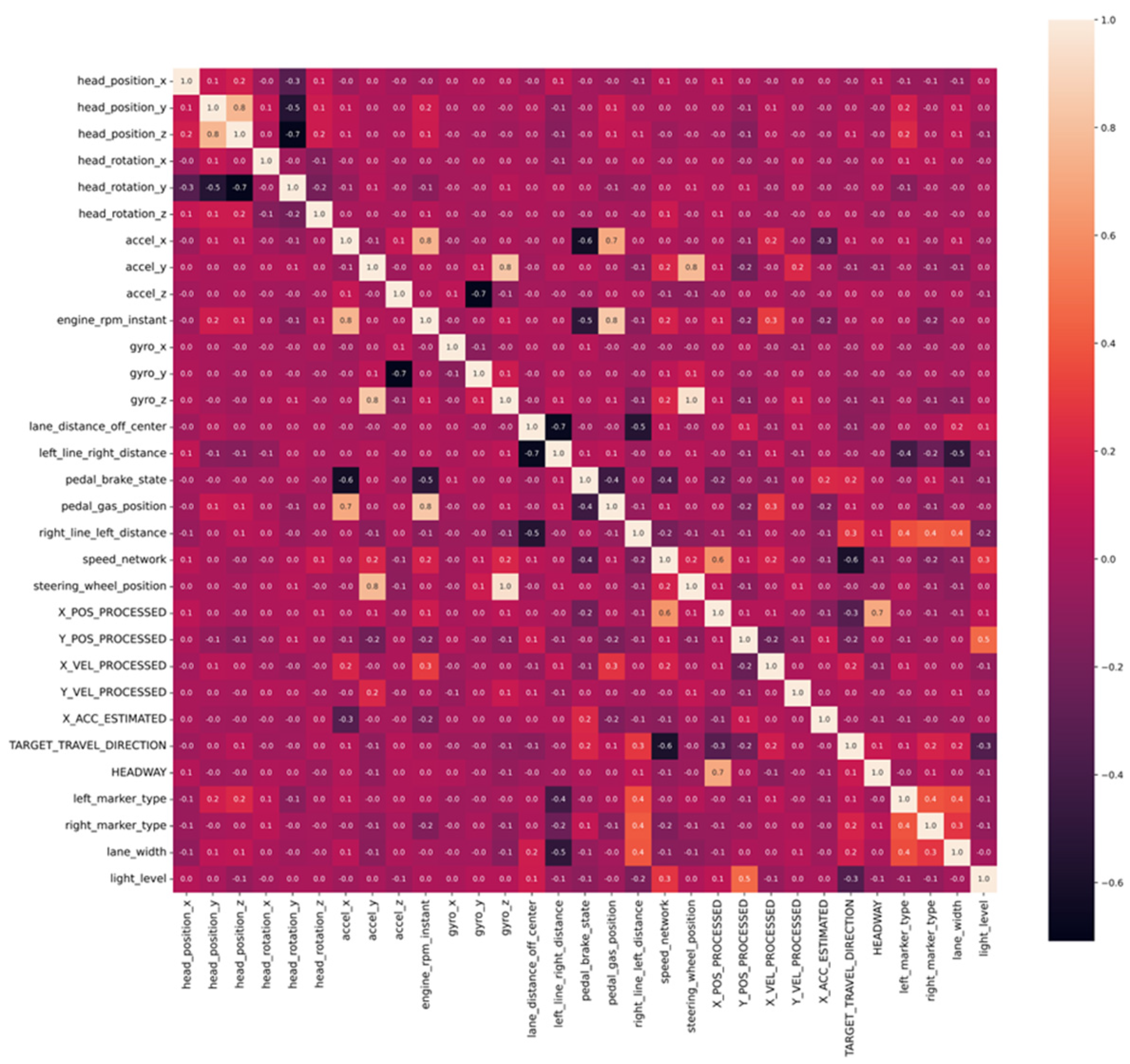
2.1. Indicator Screening and Optimization

For instance, the Highway Capacity Manual [11] defines a front time distance of 5 s or less as indicative of vehicle following. Parker [12] stipulates that a vehicle is in a following state when the critical front time value is 6 s. Traffic Flow Theory [13] considers vehicles to be in a following state if the distance between the fronts of two consecutive vehicles is within 0–100 m or 0–125 m. In China, Wang Xuesong [14] established rules for identifying following segments, specifying that the lateral offset should be less than 2.5 m, the autonomous driving speed should exceed 15 km/h, the stable following segment duration should be greater than 30 s, and the distance between the fronts of the vehicles should fall within the range of 7–120 m.

After reviewing existing criteria for extracting following behavior fragments and combining forward video, radar, and vehicle bus data, the following criteria for extracting following behavior fragments were determined:

• To ensure that both the lead and following vehicles are strictly in the same lane, the absolute value of the lateral distance is limited to 2.2 m.
• To ensure smooth traffic flow, the time distance between the fronts of the vehicles is set to be less than 5 s, the distance between the fronts of the vehicles ranges from 5 to 110 m, and the speed of the following vehicle must exceed 18 km/h.
• To ensure that the vehicle is in a stable following state, the duration of the following clip is required to be no less than 20 s.

Based on these criteria, 3222 following fragments were successfully extracted from the original data, encompassing 132 types of indicators with various characteristics. To simplify the analysis, preliminary screening was conducted to exclude irrelevant and sparse indicators.

Table 1. Results of the primary screening indicators.

Indicator Category	Index	Shorthand
Driver indicators	Y-axis head position X-axis head position	HPY HPX
	Z-axis head position	HPZ
	X-axishead rotation baseline	HRX
	Y-axis head rotation baseline	GAMES
	Z-axis head rotation baseline	HRZ
Road Parameter Metrics	Lane width	LW
	The type of left-hand lane sign for the vehicle immediately adjacent to the vehicle being used	LMT
	The type of right-hand lane sign for the vehicle immediately adjacent to the vehicle being used	RMT
Environmental indicators	Light level	LL
Vehicle operation and performance indicators	X-axis vehicle acceleration	AX
	Y-axis vehicle acceleration	AY
	Z-axis vehicle acceleration	THAT
	Instantaneous engine speed	DIFFERENT
	X-axis vehicle angular velocity	GX
	Y-axis vehicle angular velocity	GY
	Z-axis vehicle angular velocity	GZ
	Lateral distance	LDOC
	The distance from the center line of the vehicle to the inside of the left lane sign	LLRD
	The distance from the center line of the vehicle to the inside of the right lane sign	RLLD
	Pedal brake status	PBS
	Throttle opening	PGP
	Speed	SN
	Steering wheel position	SWP
	The x-axis component of the distance between the front car and the front bumper of the self car	XPP
	The y-axis component of the distance between the front car and the front bumper of the self-car	YPP
	The rate of change of the distance between the front car and the self is the x-axis component	XVP
	The rate of change of the distance between the front and self vehicles is the y-axis component	YVP
	The x-axis component of the relative acceleration of the front and self vehicles	XAE
	The direction of the vehicle in front	TTD
	The distance between the front of the car	H

presents the 31 indicators selected as the primary screening indicator dataset. Using these pre-screened indicators, the data files of each driver and vehicle were filtered, and the filtered datasets were fused. The K-nearest neighbor mean filling method was employed to address null values in the dataset, with the K value set to 2. To facilitate subsequent data analysis, the dataset was logarithmically standardized.

To avoid wasting computing power due to high correlation among metrics, it is crucial to perform correlation analysis and eliminate indicators with significant redundancy. Initially, the linear correlation between features is evaluated using the Pearson correlation coefficient method in Python. The selection process continues for driver parameters, vehicle parameters, road parameters, and environmental parameters from the initial screening, with the results depicted in Figure 1. Notably, there are eight indicators that exhibit a correlation coefficient of 0.8 or higher with other indicators. Furthermore, the nonlinear correlation of each index is assessed using the Spearman correlation coefficient method, as shown in Figure 2. The results indicate a strong nonlinear correlation between the index LDOC and the index LLRD. To refine the selection, the information entropy of the highly correlated indices is calculated. Based on the principle of information entropy retention, six indicators are re-screened: head_position_y, accel_x, gyro_z, accel_y, pedal_gas_position, and left_line_right_distance. Ultimately, these six indicators effectively capture most of the characteristics of the original data, allowing for a more concise and efficient analysis with a reduced number of indicators.

In this paper, we have chosen TTC (Time to Collision) as the quantitative metric to assess follow-up risk. To ensure the relevance of the data, we have excluded any instances where there is absolutely no follow-up risk, specifically the TTC data with negative calculated values and those exceeding 5s. The remaining data have been systematically categorized into five distinct groups through clustering analysis using the bipartite K-Means algorithm.

Table 2. Threshold range of car-following risk clustering.

Level 1 Risk (I Risk)	Level 2 Risk (II Risk)	Level 3 Risk (III Risk)	Level 4 Risk (IV Risk)	Risk-Free (No Risk)
0–1.32 s	1.32–1.90 s	1.90–2.95 s	2.95–3.98 s	>3.98 s or <0 s

presents the defined threshold ranges for the four levels of follow-up risk, as well as the indicators for non-follow-up risk.

Based on the threshold ranges established for the follow-up risk clustering, the pre-screening index dataset was divided into five categories, each representing different types of risks. These risk indicator groups at all levels were then subjected to statistical analysis and significance testing to gain insights into the underlying mechanisms of each type of indicator across various follow-up risk levels. This analysis helped in pre-selecting the input indicators for the follow-up risk identification model, with

Table 3. Optimization of parameters by grid search method.

Model	Parameter	Numeric Value
LR	Regularization intensity Tolerance	0.93 0.0005
SVM	Regularization intensity Tolerance	0.95 0.0003
KNN	Number of neighbors Number of leaf nodes	4 34
MLP	alpha The learning rate is initialized	0.0002 0.005
RF	Number of weak learners Maximum depth The minimum number of samples required for segmentation Minimum number of samples for leaf nodes Maximum number of leaf nodes	86 14 10 2 39
NB	Smooth parameters	2.00 × 10−9
XGB	Learning rate gamma Maximum depth Minimum leaf node sample weights are summed	0.025 0.06 12 3
GBDT	Learning rate Number of weak learners The minimum number of samples required for segmentation Minimum number of samples for leaf nodes Maximum depth Maximum number of leaf nodes	0.04 76 2 2 10 42

presenting the significance test results for each type of follow-up risk index.

Through a comprehensive significance test and data analysis across the four dimensions of people, vehicle, road, and environment, it was observed that several indicators showed no significant difference between the follow-up risk state and the non-tracking risk state. These include index AZ, index GY, and index YVP. Similarly, there were indicators that demonstrated no significant difference among different risk levels, namely index HRY, index HRZ, index AZ, index ERI, index GX, index PBS, index SN, index GY, index LDOC, index YVP, and index LL. These findings provide valuable insights for refining the selection of input indicators for the follow-up risk identification model.

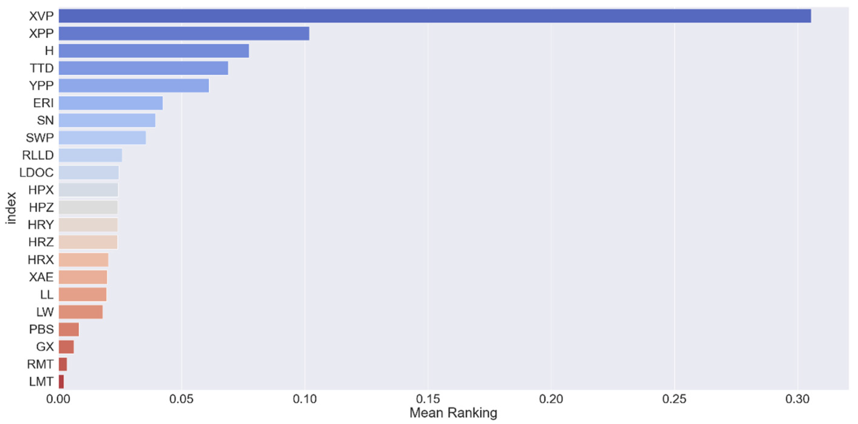
2.2. Indicator Screening Results

After excluding indicators with insignificant differences between various follow-up risk states, a large number of indicators still remain, leading to sparsity in high-dimensional space samples. This sparsity can compromise the generalization and robustness of the model, as well as prolong training times. To address this issue, this paper employs a dimensionality reduction algorithm that integrates random forest [7] and stability selection to streamline the datasets in both classification modes.

The random forest dimensionality reduction approach leverages the principles of random forest classification. It computes the mean and variance of the impurity reduction accumulation for each index variable across all trees. The variable’s importance is directly proportional to the purity reduction it achieves. Stability selection enhances this process by repeatedly applying the feature selection algorithm across different data and feature subsets. By aggregating the results of these iterations, we can derive a mean importance value for each variable across various subsets, ensuring a robust set of dimensionality-reduced features.

Based on the importance of the follow-up risk identification indicators, we calculate the cumulative contribution rate of the indicators, ranked in descending order of their importance. We then select indicators with a cumulative contribution rate exceeding 85%, while excluding those falling below this threshold. Figure 3 illustrates the ranking of risk identification indicators with and without follow-up, while Figure 4 shows the ranking for different follow-up risk levels. Notably, indicator XVP holds the highest importance, with several other indicators in the remaining blue areas also scoring high, whereas indicators in the orange areas have lower importance.

The outcomes of four rounds of index optimization and screening indicate that there are 13 indicators used to determine the presence of follow-up risk. These include XVP, XPP, H, TTD, YPP, ERI, SN, SWP, RLLD, LDOC, HPX, HPZ (of which there are 8 types), and HRY.

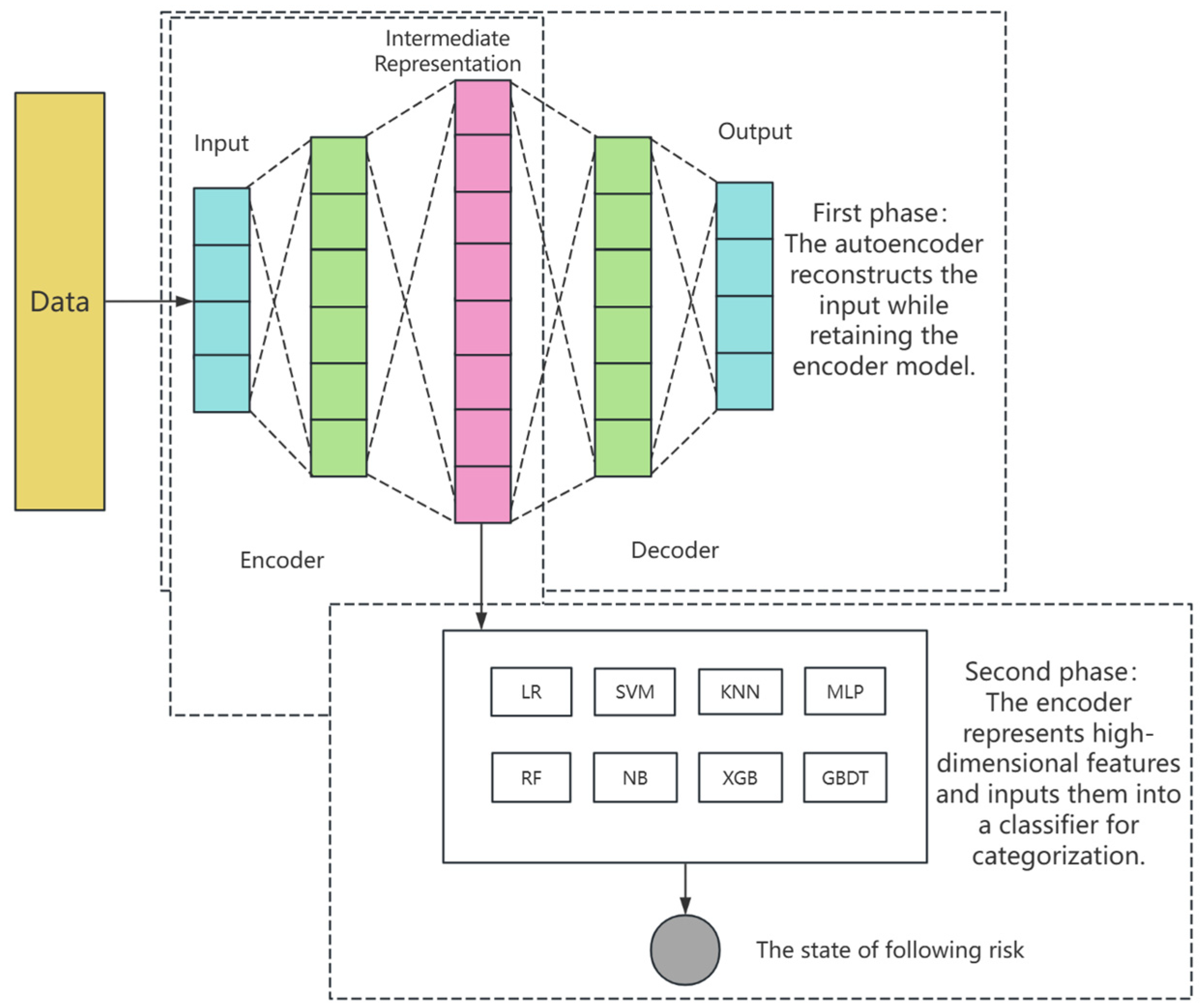
2.3. Construction of Follow-Up Risk Identification Model

The autoencoder, a neural network employed in semi-supervised and unsupervised learning, aims to perform representational learning of input information by treating it as the learning target. However, the traditional autoencoder (AE) may not guarantee the retention of essential sample characteristics. To overcome these limitations, researchers have optimized the AE, leading to the development of various advanced models such as the sparse autoencoder (SAE) [15], denoising autoencoder (DAE) [16], contractive autoencoder (CAE) [17], and the more recent variational autoencoder (VAE) [18].

In this paper, we conduct a thorough analysis of the original identification index, involving elimination, dimensionality reduction, and other operations. Ultimately, we retain indices with low correlation. Recognizing that information loss during compressed feature representation can degrade recognition accuracy, we opt for the variational autoencoder (VAE) paired with a classification algorithm for follow-up risk identification. The classification algorithm we employ encompasses Logistic Regression (LR), Support Vector Machine (SVM), K Nearest Neighbor (KNN), Multilayer Perceptron (MLP), Random Forest (RF), Naive Bayes (NB), Extreme Gradient Boosting (XGB), and Gradient Boosting Decision Tree (GBDT).

Furthermore, we enhance the autoencoder’s bottleneck layer to capture the deep features of the high-dimensional hidden space. Figure 5 illustrates the integration of the autoencoder with the classification algorithm used in this study.

The model is divided into two stages. The first stage is to input the autoencoder for the preprocessed follow-up risk identification index; the learned features are represented by the encoder layer in ascending dimension, and then the high-dimensional information in the middle layer is decoded into the same dimension as the input through the decoder layer, at this time, the loss function of the autoencoder is the root mean square error of the input and output, and the autoencoder goes through multiple rounds of iterations until the loss converges, and the encoder part is saved until the bottleneck layer is saved, and the decoder is discarded.

The goal of the autoencoder is to minimize the reconstruction error and $q(z\left|x\right.)$ the divergence between the latent variable distribution $p(z)$ and the prior distribution KL, and the objective function can be expressed as follows:

$$\tau ={\rm E}q(z\left|x\right.)\left[\log \left.p(x\left|z)\right.\right]\right.-KL(q(z\left|x\right.)‖p(z))$$

(1)

where input data, x, are denoted and latent, z, variables are described. During training, the ${\rm E}q(z\left|x\right.)\left[\log \left.p(x\left|z)\right.\right]\right.$ reconstruction error is described, and the $KL(q(z\left|x\right.)‖p(z))$ divergence between the latent variable distribution, $q(z\left|x\right.)$, and the prior distribution, p(z), is described, i.e., the distance between the two.

The input data are mapped to the mean vector, x, and the variance vector, μ, through the encoder network, σ, and the latent variables are then sampled from the distribution of the mean and variance, z, represented by the following formula:

$$\mu =f_{\mu }\left(x\right)$$

(2)

$$\sigma =f_{\sigma }\left(x\right)$$

(3)

$$z=\mu +∍\Theta \exp (\sigma /2)$$

(4)

where $\ni \in N\left(0,1\right)$, $\Theta$ represent a noise vector.

In the decoder section, you need to map the latent variables, $z$, back to the distribution, $x^{\prime }$, of the reconstructed data,$p\left(x^{\prime }|z\right)$. It is often assumed that the distribution, $x^{\prime },$ of the reconstructed data is generated by a family of distributions with a number of parameters,$Q\left(x^{\prime }|z\right)$, that are determined by the output of the decoder network. Assuming that the decoder network is a neural network with parameters,$\theta$, then the distribution of the reconstructed data can be expressed as:

$$p\left(x^{\text{'}}|z,\theta \right)=Q\left(x^{\text{'}}|z,\theta \right)$$

(5)

Define a loss function to measure the gap between the reconstructed data,$x^{\prime }$, and the original data,$x$. The loss function is expressed as the root mean square error:

$$L_{rec}(\theta )={\displaystyle \frac{1}{N}}{\displaystyle \sum _{i=1}^N{\left|x_i-x_i\text{'}\right|}^2}$$

(6)

where the $N$ number of samples is described, the original data,$x_i$, of the first sample, $i$ is described,$x_{i }^{\text{'}}$, and the reconstructed data of the first sample, $i$, is described. Since you want to minimize the reconstruction error, you need to minimize the loss function.

Finally, an end-to-end autoencoder model needs to be built by combining encoder and decoder networks. To do this, we need to define a final objective function, which is the cost function of the autoencoder:

$$L\left(\theta ,\varphi \right)=L_{rec}\left(\theta \right)+D_{KL}\left(q\varphi (z|x_i)|p(z)\right)$$

(7)

where $D_{KL}$ denotes the divergence, $KL$ denotes$q\varnothing \left(z|x_i\right)$, which is the posterior distribution of latent variables, $x_i$, calculated from the given sample, $\varnothing$, and network parameters, $z$. The cost function, $L\left(\theta ,\varnothing \right)$, is made up of the difference between the reconstruction error and the prior distribution of the latent variable, and the cost function needs to be minimized. By deriving the cost function, the backpropagation algorithm is used to train the autoencoder, update the network parameters, and minimize the cost function.

In the second stage, the identification index data are input into the trained encoder model, and the high-dimensional hidden spatial information data of the bottleneck layer output by the encoder model is input into the classifier for follow-up risk state identification training, and the trained classifier will be applied to the new data identification follow-up risk state.

3. Model Training and Validation

3.1. Model Training

The validation indicators retained in the dataset possess varying dimensions, which can potentially hinder the calculation speed during model training and validation. To mitigate this issue and expedite the computation and convergence of the model, it is imperative to standardize and normalize the dataset. Given the concentrated nature of the index data within the natural driving dataset, this study employs the max–min normalization technique to standardize the indicator dataset.

In line with the framework of the AutoEncoder_TraClassifier risk validation model proposed herein, a variational autoencoder grounded in a feedforward neural network has been constructed. Utilizing the grid search method in Python, we optimized the parameters to ascertain the optimal hyperparameters for the foundational validation model, as delineated in Table 3. These optimized parameters were then utilized to train the model.

Taking the risk validation of natural driving data with or without following as a case study, the input dimension was initially upgraded from 13 dimensions to 26 dimensions, representing the final set of retention indices for risk validation with or without following. These data were further processed to 260 dimensions in the bottleneck layer, allowing for the extraction of high-dimensional hidden space features. Subsequently, the encoder decoded these features back to their original 13 dimensions.

The sliding window method was employed to extract values from the fused time series dataset, using a window size of 2 s and a step size of 1 s. Of the dataset constructed using the sliding window method, 70% was designated as the training set, while 30% served as the test set. For training purposes, the validation index data from the first 2s was paired with the risk state of the subsequent 2s, ensuring that the risk validation model exhibited robust follow-up risk validation and prediction capabilities.

Upon completion of the autoencoder training, only the encoder portion was retained, with the bottleneck layer removed from the autoencoder. The trained autoencoder was then invoked to extract high-dimensional features from the validation index data. These high-dimensional features were subsequently fed into the eight classifier components of the AutoEncoder_TraClassifier follow-up risk validation model framework for the training and testing of each classifier.

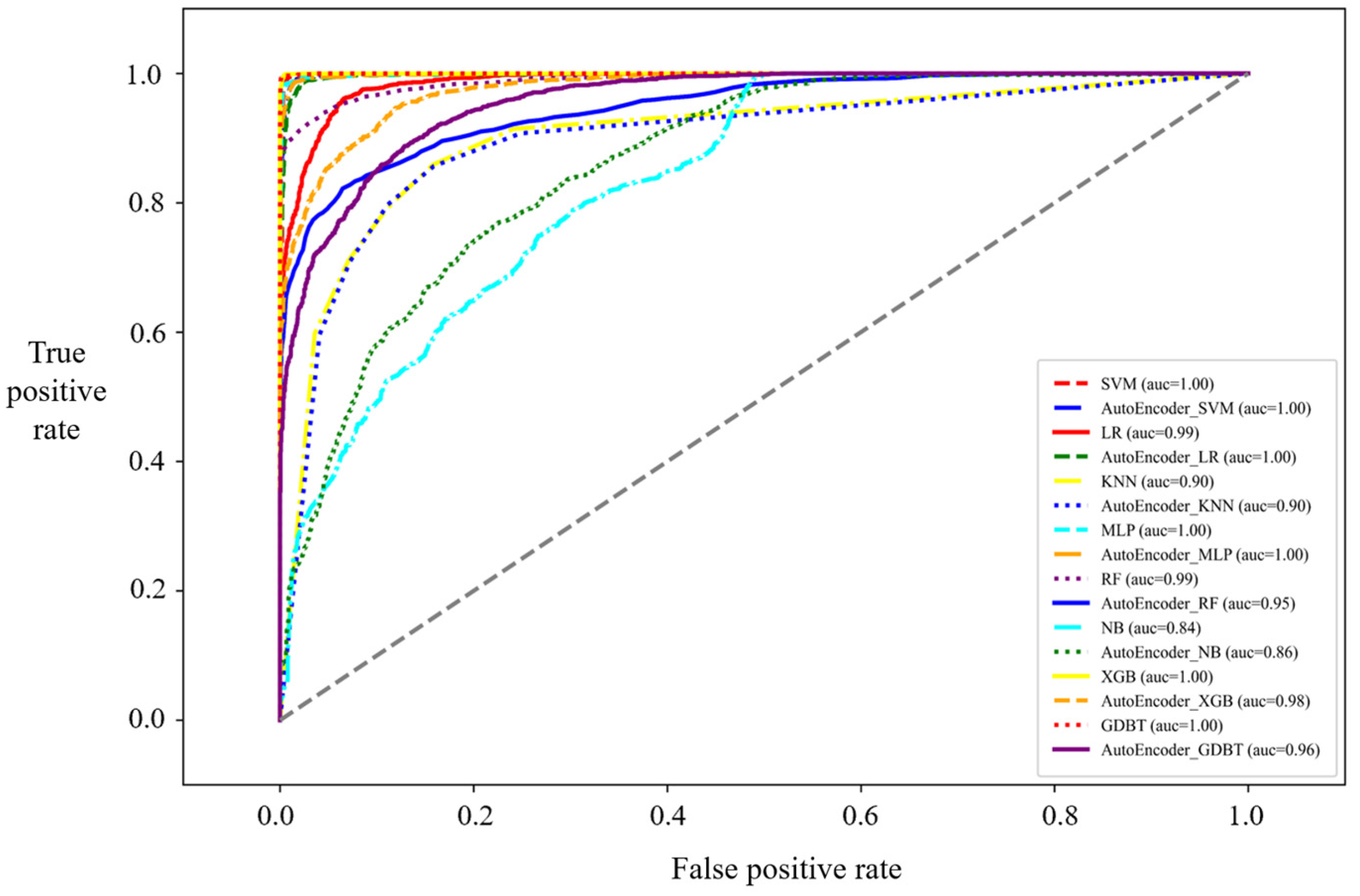
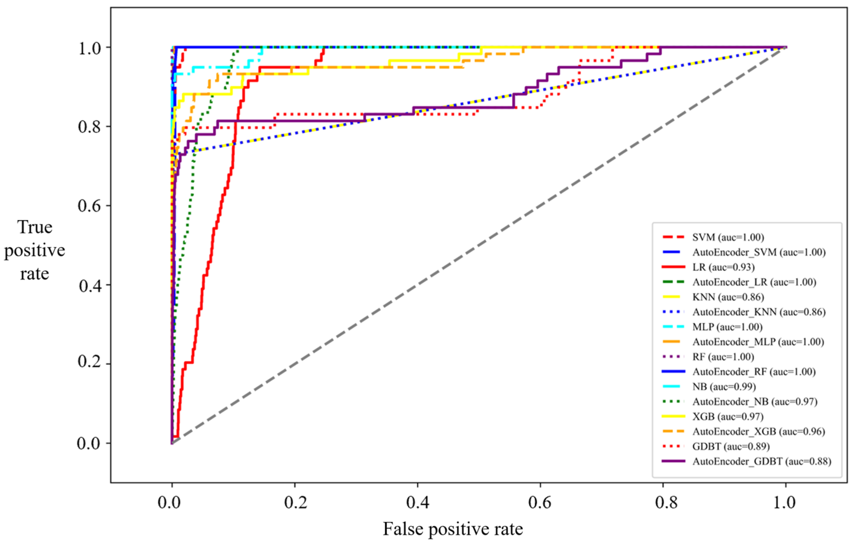
3.2. Training Results

To ensure that the AutoEncoder_TraClassifier model does not overfit, we conducted a thorough evaluation using the ROC curve analysis chart and various supervised learning assessment metrics, including accuracy, recall, precision, F1 score, and identification time, on the completed natural driving risk validation index data test set. The validation time metric represents the cumulative duration of the three-fold cross-validation training and testing phases.

(1)

Verification of Follow-up Risk Identification Model Results

Figure 6 depicts the ROC curve for risk validation with or without follow-up scenarios. Coupled with the data from other evaluation indicators presented in

Table 4. Evaluation indicators of natural driving data.

Model	Evaluation Indicators
	Accuracy	Recall	F1	Precision	Time (ms)
LR	0.8969	0.8893	0.8940	0.9123	302
AutoEncoder_LR	0.9133	0.9057	0.9108	0.9304	1871
SVM	0.8802	0.8697	0.8753	0.9082	210
AutoEncoder_SVM	0.9054	0.8971	0.9024	0.9252	4524
KNN	0.8444	0.8404	0.8404	0.8463	2980
AutoEncoder_KNN	0.8442	0.8408	0.8423	0.8451	8739
MLP	0.9016	0.8930	0.8983	0.9225	29,464
AutoEncoder_MLP	0.9149	0.9073	0.9125	0.9318	22,498
RF	0.9066	0.8982	0.9036	0.9263	5290
AutoEncoder_RF	0.8780	0.8724	0.8755	0.8849	34,673
NB	0.7149	0.7247	0.7139	0.7328	60
AutoEncoder_NB	0.7476	0.7542	0.7475	0.7562	398
XGB	0.9063	0.8980	0.9034	0.9262	2823
AutoEncoder_XGB	0.8969	0.8897	0.8941	0.9106	44,874
GDBT	0.9090	0.9009	0.9062	0.9280	9197
AutoEncoder_GDBT	0.8780	0.8721	0.8754	0.8858	247,200

, the three-fold cross-validation results indicate that when the model is not overfitted and the autoencoder strategy is not incorporated for high-dimensional feature extraction, the GDBT model achieves an accuracy of up to 90.90% on the test set among the eight validation models. Notably, the AutoEncoder_LR model attains an accuracy of 91.33%, while the AutoEncoder_MLP model reaches an accuracy of 91.49%. Furthermore, the recognition time is significantly reduced from 9197 milliseconds for the GDBT model to 1871 milliseconds for the AutoEncoder_LR model, thereby enhancing both the accuracy and recognition speed of the validation models.

The strategy of incorporating an autoencoder to extract high-dimensional recognition features into eight basic recognition models reveals a pattern: while the recognition time increases, certain models demonstrate superior risk-free recognition performance in natural driving data. Specifically, the LR model, SVM model, MLP model, and NB model maintain or improve their performance. Conversely, the RF model, XGB model, and GDBT model show decreased performance. The KNN model’s performance remains largely unchanged. This discrepancy can be attributed to the fact that ensemble models, such as tree-based models, struggle to effectively partition the feature space of high-dimensional data, leading to suboptimal results. In contrast, models like the LR model benefit from their inherent regularization terms, which help reduce overfitting and enhance the model’s generalization and robustness. Notably, the AutoEncoder_LR model combines high accuracy, low latency, and excellent real-time performance, making it a suitable choice for both follow-up and non-follow-up risk validation scenarios.

(2)

Analysis of Validation Model Results for Different Follow-up Risk Levels

Figure 7 illustrates the ROC curve for different levels of follow-up risk, complemented by the evaluation index data presented in

Table 5. Evaluation indicators validation model group of different car-following risk level.

Model	Evaluation Indicators
	Accuracy	Recall	F1	Precision	Time (ms)
LR	0.5765	0.3471	0.3412	0.3886	1049
AutoEncoder_LR	0.7014	0.5497	0.5986	0.7402	3232
SVM	0.6232	0.4144	0.4096	0.4303	523
AutoEncoder_SVM	0.6781	0.4809	0.5114	0.7108	21,011
KNN	0.6735	0.5046	0.5467	0.7019	1500
AutoEncoder_KNN	0.6735	0.5045	0.5480	0.7141	7318
MLP	0.7101	0.5176	0.5520	0.7421	20,396
AutoEncoder_MLP	0.6891	0.5492	0.5999	0.7315	36,435
RF	0.6781	0.4972	0.5375	0.7153	3936
AutoEncoder_RF	0.6787	0.4916	0.5288	0.7156	24,601
NB	0.5934	0.4654	0.4802	0.6299	58
AutoEncoder_NB	0.5809	0.4970	0.4484	0.4361	409
XGB	0.6923	0.5320	0.5789	0.7302	8505
AutoEncoder_XGB	0.6806	0.5083	0.5515	0.7169	111,974
GDBT	0.6883	0.5054	0.5447	0.7224	30,786
AutoEncoder_GDBT	0.6732	0.5324	0.5773	0.7032	755,456

. The results indicate that validating various levels of follow-up risk is more challenging than distinguishing between the presence or absence of follow-up risk. However, the performance trends among the models are similar to those observed in the risk validation models for follow-up scenarios. The LR model and SVM model stand out as they improve the performance of the validation model on natural driving data. Conversely, the MLP model, NB model, XGB model, and GDBT model show decreased performance. The KNN model and RF model maintain their performance levels. Among the basic validation models, the AutoEncoder_LR model achieves the highest accuracy of 70.14%, surpassing the MLP model’s accuracy of 70.01% by 0.18%. Moreover, the AutoEncoder_LR model accelerates the validation process by 84.15%.

3.3. Model Validation

After employing the processed data and the method of model training and testing to validate the following risk validation model, Figure 8 presents the ROC curve used to evaluate whether the simulated driving data, when analyzed together with the data provided in

Table 6. Evaluation index of validation models of whether there is car-following risk by using simulated driving data.

Model	Evaluation Indicators
	Accuracy	Recall	F1	Precision	Time (ms)
LR	0.8986	0.9044	0.8984	0.9109	1280
AutoEncoder_LR	0.9576	0.9583	0.9575	0.9570	3223
SVM	0.9009	0.9066	0.9008	0.9126	686
AutoEncoder_SVM	0.9370	0.9406	0.9370	0.9405	11,688
KNN	0.8610	0.8638	0.8609	0.8631	14,292
AutoEncoder_KNN	0.8589	0.8616	0.8589	0.8609	33,733
MLP	0.9008	0.9065	0.9007	0.9126	54,108
AutoEncoder_MLP	0.9505	0.9534	0.9505	0.9522	116,309
RF	0.9012	0.9069	0.9011	0.9129	18,794
AutoEncoder_RF	0.8809	0.8845	0.8809	0.8848	136,306
NB	0.7942	0.7888	0.7903	0.8009	77
AutoEncoder_NB	0.8409	0.8343	0.8368	0.8562	1000
XGB	0.8951	0.9012	0.8949	0.9086	3455
AutoEncoder_XGB	0.8897	0.8948	0.8896	0.8987	64,089
GDBT	0.9188	0.9235	0.9187	0.9262	37,384
AutoEncoder_GDBT	0.9007	0.9023	0.9006	0.9008	796,193

, contains subsequent risks.

When compared to the natural driving data, the simulated driving data demonstrate improvements in validation accuracy, recall, precision, and F1 score. Notably, the accuracy can reach up to 95.76%. Furthermore, the performance trends of each recognition model after incorporating the autoencoder strategy remain consistent with those observed in natural driving data.

Specifically, the models that exhibit enhanced risk validation performance on simulated driving data include the LR model, SVM model, MLP model, and NB model. Conversely, the XGB model, GDBT model, and RF model show decreased performance. The KNN model maintains its performance, indicating minimal change. These findings suggest that the risk validation model possesses good generalization and robustness, as evidenced by its consistent performance across different datasets.

Figure 9 depicts the ROC diagram for assessing the risk of following in simulated driving data. When analyzed in conjunction with the data presented in

Table 7. Evaluation index of validation models of different car-following risk level by using simulated driving data.

Model	Evaluation Indicators
	Accuracy	Recall	F1	Precision	Time (ms)
LR	0.5967	0.3677	0.3617	0.4087	2174
AutoEncoder_LR	0.7153	0.5822	0.6334	0.7564	5899
SVM	0.5919	0.3879	0.3755	0.4015	1185
AutoEncoder_SVM	0.6709	0.5775	0.6169	0.6883	60,323
KNN	0.6832	0.5502	0.5979	0.7138	3236
AutoEncoder_KNN	0.6787	0.5453	0.5941	0.7190	27,326
MLP	0.6978	0.6059	0.6513	0.7472	43,833
AutoEncoder_MLP	0.7381	0.7290	0.7616	0.8077	45,797
RF	0.7145	0.6079	0.6587	0.7605	7803
AutoEncoder_RF	0.6966	0.5888	0.6392	0.7453	54,599
NB	0.6045	0.4811	0.5028	0.6449	94
AutoEncoder_NB	0.5872	0.4967	0.4920	0.5220	769
XGB	0.7138	0.6369	0.6854	0.7695	14,916
AutoEncoder_XGB	0.6911	0.5780	0.6284	0.7393	185,558
GDBT	0.6605	0.5540	0.6044	0.7217	56,182
AutoEncoder_GDBT	0.6443	0.4966	0.5430	0.6913	2,168,225

, it becomes evident that the simulated driving data outperforms the natural driving data overall. Moreover, the performance trends of the models in this simulation test align with their ability to identify the presence of a following risk.

Specifically, the models that demonstrate varying degrees of improvement in verifying follow-up risk in simulated driving data are the LR model, SVM model, and MLP model. Conversely, the models that show decreased performance include the XGB model, GDBT model, RF model, and NB model. Notably, the KNN model maintains its performance, which is consistent with its performance in natural driving data. This indicates that each recognition model possesses good generalization and robustness.

Additionally, the AutoEncoder_LR model achieves an accuracy improvement of 0.11% compared to the highest accuracy of 71.45% achieved by the RF model in the basic recognition model. Furthermore, the recognition time of the AutoEncoder_LR model is accelerated by 24.40%. These findings suggest that the AutoEncoder_LR model offers a more efficient and accurate approach for verifying follow-up risks in simulated driving data.

To summarize, under the four combinations of the autoencoder strategy, the LR model and SVM model consistently show stable improvements in the performance of following risk validation. Conversely, the RF model, XGB model, and GDBT model experience decreased performance. The KNN model maintains basically unchanged performance, while the NB model and MLP model exhibit unstable performance changes. Ultimately, the AutoEncoder_LR model is selected as the final follow-up risk validation model. Figure 10 is a framework diagram for model training and validation.

4. Collision Avoidance Grading Early Warning Strategies

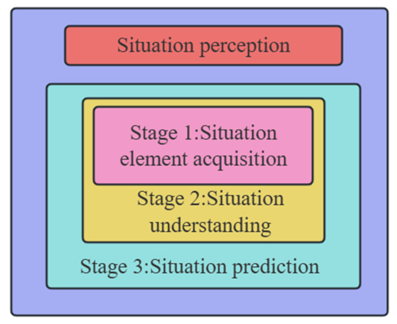
4.1. Situational Awareness Framework

As illustrated in Figure 11, acquiring situational elements involves extracting the pivotal factors that impact the safety of the target observation system within a specific network environment. Situation understanding entails the integration and analysis of the collected data, culminating in the presentation of analytical results. This process includes reducing the dimensionality of selected natural driving characteristics, utilizing saliency analysis, and other methodologies to identify high-risk influencing factors, which is akin to gaining an understanding of the situation. Furthermore, situation understanding involves modeling and analyzing the indicator system. Situation forecasting, on the other hand, builds upon the outcomes of situation understanding to conduct a deeper analysis and prediction of the future state and development trend of the system.

The three-tier model of situational awareness serves as a comprehensive framework for analyzing, identifying, predicting, responding to, and managing risks from a global perspective, ultimately guiding decision making and actions. This model embodies the application of risk identification technology. Within this framework, acquiring natural driving source data constitutes the foundational layer. The core lies in processing and analyzing current data through the utilization of a sophisticated risk identification model that has been constructed. The crucial aspect involves predicting real-time potential risks and making timely warning decisions based on the model’s identification and prediction outcomes. Leveraging the research findings from the first two stages—situation element acquisition and situation understanding—a vehicle dynamics model was chosen to accomplish the task of situation prediction.

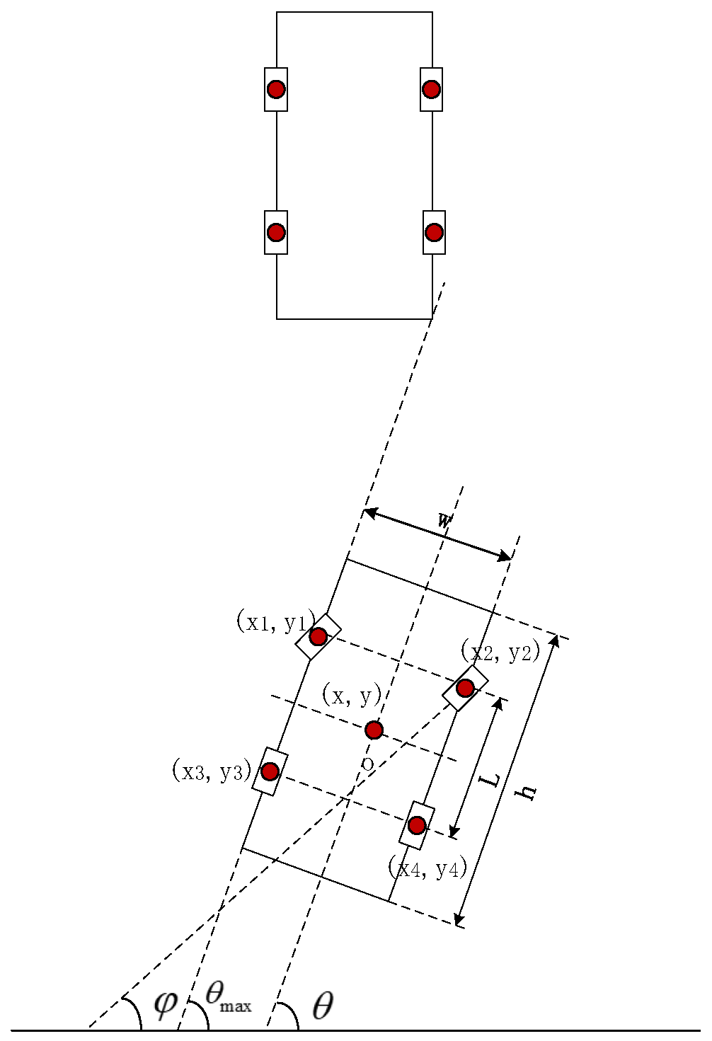
4.2. Vehicle Dynamics Motion Analysis

4.2.1. Vehicle Dynamics Model Construction

The risk warning strategy examined in this study is specifically tailored for scenarios where the driver remains within their current lane. However, in situations where the driver maintains a following distance but intends to change lanes, accurately capturing the vehicle’s real-time motion state becomes challenging due to the reliance of the constructed identification model on a combination of multi-source heterogeneous indicators. Therefore, to predict the vehicle’s trajectory at the next moment, it is necessary to integrate the vehicle dynamics model.

The vehicle dynamics model offers a scientific and accurate representation of the vehicle’s motion laws, boasting excellent real-time performance. In this study, based on the classical two-degree-of-freedom transverse dynamics model, we opt for a simplified rectangular model that balances precision and abstraction. The vehicle is abstracted as a rectangle, where the length corresponds to the actual length of the vehicle and the width matches its actual width. The kinematic state function of the vehicle can be expressed as follows:

$$X(t)={(x,y,h,w,L,v,\theta ,\phi )}^T$$

(8)

The $x$ and $y$positions are coordinates of the vehicle in the following state;$h$ is the length of the vehicle; $w$ is the width of the vehicle;$L$is the distance between the front axle of the vehicle and the rear axle of the vehicle; $v$ is the speed; $\theta$is the instantaneous heading angle of the vehicle; is the $\phi$steering angle of the front wheel of the vehicle. The vehicle motion model is shown in Figure 12:

According to the relationship between angular velocity, linear velocity and radius in curvilinear motion, the distance between the front and rear axles,$L$, is the radius of the vehicle during turning, and the following formula can be obtained:

$$\omega ={\displaystyle \frac{v\tan \phi }{L}}$$

(9)

where is the $\omega$ instantaneous angular velocity of the vehicle. From this, we can obtain the equation for the state of motion of the vehicle according to the kinematic relationship as follows:

$$\left\{\begin{array}{l}{\displaystyle \frac{d\theta }{dt}}={\displaystyle \frac{v\tan \phi }{L}}\\ {\displaystyle \frac{dx}{dt}}=v\cos \theta \\ {\displaystyle \frac{dy}{dt}}=v\sin \theta \end{array}\right.$$

(10)

Converted into integral form, as follows:

$$\left\{\begin{array}{l}\theta ={\displaystyle {\int }_t^{t+\Delta t}\frac{v\tan \phi }{L}}\\ \Delta x={\displaystyle {\int }_t^{t+\Delta t}v\cos \theta }\\ \Delta y={\displaystyle {\int }_t^{t+\Delta t}v\sin \theta }\end{array}\right.$$

(11)

$\Delta x, \Delta y$ is the distance traveled by the vehicle on the horizontal and vertical axes, and then the position coordinates of the vehicle at the next moment are:

$$\left\{\begin{array}{l}{x}_t=x_{t-1}+\Delta x\\ y_t=y_{t-1}+\Delta y\end{array}\right.$$

(12)

Through continuous iterative calculations, we can determine the vehicle’s position at the next moment based on its position and motion state from the previous moment. Additionally, the vehicle’s motion state can be predicted in this manner. According to the driving risk identification model constructed for the following scenario, once the vehicle enters the risk range, the early warning strategy will instantly predict the vehicle’s movement state at the next moment. Subsequently, the system will proceed to the judgment stage to assess the vehicle’s following state.

4.2.2. Determination of Vehicle Following Status

The vehicle dynamics model can predict the movement state of the vehicle at the next moment in real time, so it is necessary to determine whether the vehicle has the intention to change lanes when following the risk according to the vehicle kinematics module, so as to determine the early warning strategy of the response and reduce false warning. Figure 13 is a schematic diagram of vehicle following motion, the upper rectangular model represents the car in front, and the heading angle of the car relies on GPS equipment to observe; if the heading angle of the car $\theta$continues to be less than the maximum heading angle, ${\theta }_{max}$, it is judged that the vehicle has the intention to change lanes, and the system does not send out an early warning prompt. In addition, when the system determines that there is a risk of following, if the speed collected by the speed sensor still maintains the current speed or continues to increase, the system will issue an early warning.

According to Zhu Xichan’s study on the potential risk classification standard in the following state, 2s was used as the safety margin value for dividing the hazard domain. If the speed of the vehicle continues to drop beyond the risk range within 2s, the system will not warn. Figure 14 shows the overall judgment process of the vehicle following state.

4.3. Early Warning Grading Information Prompt Design

From the current domestic and international scenarios, it is evident that auditory warnings, despite being susceptible to environmental noise, are readily perceived by drivers. They offer rapid recognition speeds and shorter reaction times. Additionally, auditory warnings do not obstruct the driver’s field of vision and have a relatively minor impact on their driving experience. In comparison to visual and tactile warnings, auditory warnings present a more convenient and mature form of alerting. Therefore, this paper selects auditory warnings as the primary method for issuing early warnings.

In contemporary research, auditory early warning methods can broadly be categorized into four types: abstract sound cues, analog sound cues, music cues, and voice information. Abstract sounds, such as “didi” and “beep”, necessitate minimal response time and exhibit a strong warning effect, making them a popular choice for advanced driver assistance systems. While both analog sounds and music can promptly alert drivers, analog sounds may confuse drivers by mimicking real-world sounds, and music can potentially affect a driver’s physiology and psychology. Furthermore, the vast selection range of analog sounds and music hinders their practical application. Voice cues, commonly used in in-vehicle systems like voice assistants and map navigation, resemble abstract sounds in functionality. Hence, this early warning strategy opts for abstract sounds as the auditory warning method. Based on the index optimization screening process outlined in Section 3, eight key indicators with the highest final importance for identifying following risk levels were selected and integrated into the driving risk identification model constructed in Section 3 to ascertain the vehicle’s risk level.

Given the distinct early warning characteristics of auditory, tactile, and visual warning methods, a composite warning scheme that primarily relies on auditory warnings, supplemented by visual and tactile cues, is proposed. This scheme, detailed in

Table 8. Design of early warning scheme based on “visual-auditory-tactile”.

Risk Level	Level 1 Risk	Level 2 Risk	Level 3 Risk	Level 4 Risk
Urgency	Particularly urgent	Highly urgent	Moderately urgent	Low-severity emergency
Visual warning	-	red light	red light	Red light or flashing
Auditory warning	High-frequency “drip” sound	High-frequency “drip” sound	“Didi” sound	-
Tactile warning	The steering wheel vibrates	-	-	-

, aims to harness the strengths of these three warning methods to enhance the overall effectiveness of early warnings.

• When the vehicle is at the lowest risk level, which is the fourth level, a red light warning will be displayed on the screen for 2 s, ensuring that it does not distract or disrupt the driver’s vision. If the vehicle is at the third risk level, both a red light warning and an audible “Didi” sound will be utilized for a duration of 2 s. At the second risk level, a red light warning accompanied by a high-frequency “Didi” sound will be employed for 2s. When the vehicle is at the highest risk level, the visual warning method may gradually become ineffective and occupy the driver’s cognitive time. To avoid adverse effects, a high-frequency “Didi” sound and steering wheel vibration will be used for 2 s instead.
• If the vehicle is at the first risk level and maintains a constant speed or continues to accelerate, an auditory-tactile combined warning prompt will be activated, along with a speed suggestion. However, if the vehicle decelerates and reaches a risk-free state within 2 s, no warning prompt will be displayed. If it does not, the corresponding prompt will appear when it slows down to the second, third, or fourth risk levels.
• When the vehicle is at the second risk level and maintains a constant speed or accelerates, a visual-high-frequency “Didi” sound and auditory combined warning prompt will be given, along with a speed suggestion. If the vehicle decelerates and reaches a risk-free state within 2 s, no warning will be issued. If it does not, the corresponding prompt will appear when it slows down to the third or fourth risk levels.
• If the vehicle is at the third risk level and maintains a constant speed or accelerates, a visual and auditory “Didi” combined sound warning prompt will be used to provide speed suggestions. If the vehicle decelerates and reaches a risk-free state within 2 s, no warning prompt will be displayed. If it does not, a corresponding prompt will appear when it slows down to the fourth risk level.
• When the vehicle is at the fourth risk level and maintains a constant speed or accelerates, a red light flashing visual warning prompt will be displayed, along with speed suggestions. If the vehicle decelerates and reaches a risk-free state within 2 s, no warning prompt will be issued. If it does not, a warning corresponding to the fourth risk level will be displayed.

4.4. Potential Effect on User Groups

(1)

Positive Behavioral Change:

Users who regularly rely on these strategies may develop safer habits and behaviors over time, incorporating them into their daily routines. This behavioral shift can lead to a reduction in accidents and incidents, fostering a safer environment for everyone.

(2)

Trust and Confidence in Technology:

Effective implementation of collision avoidance grading early warning strategies can bolster users’ trust in technology and its ability to enhance safety. This trust can encourage wider adoption of similar technologies, driving further innovation and improvement in safety systems.

(3)

Economic Benefits:

By reducing accidents and associated costs (e.g., medical expenses, property damage, legal fees), these strategies can have significant economic benefits for individuals, businesses, and society at large. They can also contribute to a more sustainable environment by minimizing the environmental impact of accidents, such as oil spills or hazardous material spills.

(4)

Regulatory Compliance and Standards:

As safety regulations and standards continue to evolve, collision avoidance grading early warning strategies can help users comply with new requirements. This compliance can be particularly important in industries where safety is heavily regulated, such as aviation, maritime, and construction.

5. Potential Limitations

(1)

Data Quality and Accuracy:

The accuracy and reliability of the model depend heavily on the quality and accuracy of the input data. Errors or inconsistencies in data sources can directly impact the model’s predictions and reliability.

(2)

Data Privacy and Security:

Multi-source information fusion involves integrating data from multiple sources, potentially including sensitive or personal information. Strict adherence to relevant laws, regulations, and privacy policies is crucial to ensure data legality and security. Technical measures such as data encryption and access control are necessary to prevent data breaches and misuse.

(3)

Model Complexity and Computational Cost:

The model is often complex, requiring significant computational resources to process large volumes of data and complex algorithms. This can increase computational costs and limit its application in scenarios requiring high real-time performance. Optimization of model structure and algorithms is essential to improve computational efficiency and real-time performance.

(4)

Model Interpretability and Understandability:

The complexity of multi-source information fusion can make the model less interpretable and understandable. This can affect its adoption and acceptance in practical applications. Efforts should be made to enhance the model’s interpretability and understandability to facilitate user comprehension and acceptance.

(5)

Dependency and Robustness:

The model relies on multiple data sources for input. Failures or data loss in any source can affect the model’s operation and accuracy. Effective data backup and recovery mechanisms, as well as strategies for handling data missingness and anomalies, are crucial to improve the model’s robustness and reliability.

(6)

Insufficient conditions

Due to insufficient conditions for conducting experiments on real roads, there may be a gap between the accuracy of the model and reality, specifically manifesting as: decreased model prediction accuracy, insufficient model generalization ability, accuracy issues caused by data bias, improper adjustment of model parameters, and sensor and algorithm limitations. In practical applications, it is still necessary to continuously collect and analyze data to optimize and improve the model.

6. Discussion

In order to determine the effectiveness of our suggested methodology, we compare the performance of follow-up risk identification model with other, comparable methods in this section. The seven papers chosen for this purpose are as follows:

• Ref [19]: A study on traffic conflict prediction model of closed lanes on the outside of expressway involves analyzing various factors that contribute to potential traffic conflicts in scenarios where lanes on the outer side of an expressway are closed.
• Ref [20]: Research on characteristics and trends of traffic flow based on the mixed velocity method and background difference method offers significant potential for improving the understanding of traffic behavior and optimizing road networks.
• Ref [21]: Fusing near-infrared and Raman spectroscopy coupled with deep learning LSTM algorithm represents a powerful tool for analyzing and predicting the properties and behavior of materials. This technique has wide applications in various fields.
• Ref [22]: In the realm of traffic engineering and highway safety, the determination of warning zone lengths on freeways is a critical task. These warning zones play a vital role in alerting drivers to potential hazards or changes in traffic conditions ahead, thereby enabling them to take necessary precautions and avoid accidents.
• Ref [23]: The CNN-LSTM approach combines the feature extraction capabilities of CNNs with the time series modeling capabilities of LSTMs, making it a powerful tool for handling and predicting time series data.
• Ref [24]: Video-based deep learning methods are powerful tools for processing and analyzing video data.
• Ref [25]: The Improved TTC Algorithm represents a significant advancement in traffic conflict detection and prediction. By addressing the limitations of the traditional TTC algorithm and incorporating additional factors and techniques, it provides a more accurate and reliable method for detecting potential rear-end conflicts in complex traffic environments.

It is worth noting that although these papers use the LSTM, TTC and LSTM-CNN algorithms, the characteristics of the data and the objectives of the research are different. Nonetheless, we compared the RMSE value of our method with these methods. Our proposed method outperformed all the methods, having the lowest RMSE value.

7. Conclusions

In this study, an AutoEncoder_TraClassifier following a risk validation model is constructed based on a deep feedforward neural network autoencoder, aiming to enhance driving safety and reduce the incidence of rear-end collision accidents. The experimental results indicate that, despite variations in the performance of different recognition models after integrating the autoencoder strategy, the performance trends of each model align consistently with the validation results from both simulated tests with and without the risk of following. Furthermore, the performance of each model remains consistent with its performance in natural driving data, suggesting good generalization and robustness.

Compared to the basic validation model, the AutoEncoder_LR model exhibits improvements in accuracy, recall, precision, and F1 score. Additionally, it offers the advantages of high accuracy, low latency, and high real-time performance. However, it should be noted that this study used driving simulation tests for model verification. Given the complexity and variability of real-world road conditions, as well as potential simulation errors, future work should involve real vehicle verification.

References

1. Traffic Management Bureau of the Ministry of Public Security. There Are 435 Million Vehicles, 523 Million Drivers, and More than 20 Million New Energy Vehicles in China; Traffic Management Bureau of the Ministry of Public Security: Beijing, China, 2023. [Google Scholar]
2. National Bureau of Statistics. China Statistical Yearbook 2023; National Bureau of Statistics: Beijing, China, 2023. [Google Scholar]
3. Yang, Z. Research on Causes of Rear-End Collision and Behavior of Avoiding Collision Based on Deep Data Analysis; Northeast Forestry University: Harbin, China, 2021. [Google Scholar]
4. Tan, J.H. Impact of risk illusions on traffic flow in fog weather. Physica A Stat. Mech. Appl. 2019, 525, 216–222. [Google Scholar] [CrossRef]
5. Liu, Z.H.; Zhang, K.D.; Ni, J. Analysis and Identification of Drivers’ Difference in Car-Following Condition Based on Naturalistic Driving Data. J. Transp. Syst. Eng. Inf. Technol. 2021, 21, 48–55. [Google Scholar]
6. Bai, Y.; Ren, M.H. Improving Car Following Model Before the Vehicle Changes Lanes Based on NGSIM Data. Traffic Transp. 2023, 39, 25–29. [Google Scholar]
7. Huang, Z.G.; Guo, X.C.; Jia, L. Car-Following Risk Behavior in Rainy Weather Based on Random Forest. J. Transp. Inf. Saf. 2020, 38, 27–34. [Google Scholar]
8. Hjelkrem, A.O.; Ryeng, O.E. Chosen risk level during car-following in adverse weather conditions. Accident Anal. Prev. 2016, 95, 268–275. [Google Scholar] [CrossRef]
9. Ge, H.; Bo, Y.; Zang, W.; Zhou, L.; Dong, L. Literature review of driving risk identification research based on bibliometric analysis. J. Traffic Transp. Eng. (Engl. Ed.) 2023, 3, 118–130. [Google Scholar] [CrossRef]
10. Wang, M.; Tu, H.Z.; Li, H. Prediction of Car-Following Risk Status Based on Car-Following Behavior Spectrum. J. Tongji Univ. (Nat. Sci.) 2021, 49, 843–852. [Google Scholar]
11. Transportation Research Board (TRB). Highway Capacity Manual 2010; Highway Research Board: Washington, DC, USA, 2010. [Google Scholar]
12. Paker, M. The Effect of Heavy Goods Vehicles and Following Behavior on Capacity at Motorway Roadwork Sites. Traffic Eng. Control 1996, 37, 524–531. [Google Scholar]
13. Gartner, N.; Messer, C.J.; Raathi, A.K. Traffic Flow Theory (Update of TRB Special Report 1165); Transportation Research Board: Washington, DC, USA, 1997. [Google Scholar]
14. Wang, X.S.; Zhu, M.X. Calibrating and Validating Car-Following Models on Urban Expressways for Chinese Drivers Using Naturalistic Driving Data. China J. Highw. Transp. 2018, 31, 129–138. [Google Scholar]
15. Ng, A. Sparse Autoencoder. CS294A Lect. Notes 2011, 72, 1–19. [Google Scholar]
16. Vincent, P.; Larochelle, H.; Lajoie, I.; Bengio, Y.; Manzagol, P.A.; Bottou, L. Stacked denoising autoencoders: Learning useful representations in a deep network with a local denoising criterion. J. Mach. Learn. Res. 2010, 11, 3371–3408. [Google Scholar]
17. Rifai, S.; Vincent, P.; Muller, X.; Glorot, X.; Bengio, Y. Contractive auto-encoders: Explicit invariance during feature extraction. In Proceedings of the 28th International Conference on Machine Learning, Bellevue, WA, USA, 28 June–2 July 2011; Omnipress: Bellevue, WA, USA, 2011; pp. 833–840. [Google Scholar]
18. Kingma, D.P.; Welling, M. Auto-Encoding Variational Bayes. In Proceedings of the International Conference on Learning Representations (ICLR), Scottsdale, AZ, USA, 2–4 May 2013. [Google Scholar]
19. Ge, H.; Huang, M.; Lu, Y.; Yang, Y. Study on Traffic Conflict Prediction Model of Closed Lanes on the Outside of Expressway. Symmetry 2020, 12, 926. [Google Scholar] [CrossRef]
20. Ge, H.; Sun, H.; Lu, Y. Research on Characteristics and Trends of Traffic Flow Based on Mixed Velocity Method and Background Difference Method. Math. Probl. Eng. 2020, 2020, 1–9. [Google Scholar] [CrossRef]
21. Nunekpeku, X.; Zhang, W.; Gao, J.; Adade, S.Y.S.S.; Chen, Q. Gel Strength prediction in ultrasonicated chicken mince: Fusing near-infrared and Raman spectroscopy coupled with deep learning LSTM algorithm. Foods 2024, 14, 168. [Google Scholar] [CrossRef]
22. Ge, H.; Yang, Y. Research on Calculation of Warning Zone Length of Freeway Based on Micro-Simulation Model. IEEE Access 2020, 8, 76532–76540. [Google Scholar] [CrossRef]
23. Wang, Y.; Li, T.; Chen, T.; Zhang, X.; Taha, M.F.; Yang, N.; Shi, Q. Cucumber Downy Mildew Disease Prediction Using a CNN-LSTM Approach. Agronomy 2024, 14, 1155. [Google Scholar] [CrossRef]
24. Chen, C.; Zhu, W.; Steibel, J.; Siegford, J.; Han, J.; Norton, T. Classification of drinking and drinker-playing in pigs by a video-based deep learning method. Animals 2020, 196, 1–14. [Google Scholar] [CrossRef]
25. Ge, H.; Xia, R.; Sun, H.; Yang, Y.; Huang, M. Construction and Simulation of Rear-End Conflicts Recognition Model Based on Improved TTC Algorithm. IEEE Access 2019, 7, 134763–134771. [Google Scholar] [CrossRef]
Figure 1. Matrix of linear correlation coefficient of indicators.
Systems 13 00041 g001
Figure 2. Matrix of nonlinear correlation coefficient of the index.
Systems 13 00041 g002
Figure 3. Ranking chart of the importance of risk identification indicators with or without follow-up.
Systems 13 00041 g003
Figure 4. Ranking chart of the importance of different follow-up risk level identification indicators.
Systems 13 00041 g004
Figure 5. AutoEncoder_TraClassifier car-following risk identification model framework.
Systems 13 00041 g005
Figure 6. ROC diagram of risk validation with or without following in natural driving data.
Systems 13 00041 g006
Figure 7. ROC diagram of different following risk level validation models for natural driving data.
Systems 13 00041 g007
Figure 8. Validation of ROC diagram of simulated driving data with or without following risk.
Systems 13 00041 g008
Figure 9. ROC diagram of different following risks of simulated driving data.
Systems 13 00041 g009
Figure 10. Frame diagram on model training and validation.
Systems 13 00041 g010
Figure 11. Situational Awareness Framework Diagram.
Systems 13 00041 g011
Figure 12. Schematic diagram of the vehicle motion model.
Systems 13 00041 g012
Figure 13. Schematic diagram of vehicle following motion.
Systems 13 00041 g013
Figure 14. The process of determining the following status of the vehicle.
Systems 13 00041 g014