1. Introduction
Any system—engineering, natural, biological, or social—is considered adaptive if it can maintain its performance, or survive in spite of large changes in its environment or in its own components. In contrast, small changes or small ranges of change in system structure or parameters can be treated as system uncertainty, which can be remedied in dynamic operation either by the static process of design or the design of feedback and feed-forward control systems. By systems, we mean those in the sense of classical mechanics. The knowledge of initial conditions and governing equations determines, in principle, the evolution of the system state or degrees of freedom (a rigid body for example has twelve states–three components each of position, velocity, orientation and angular velocity). All system performance, including survival or stability, is in principle expressible as functions or functionals of system state. The maintenance of such performance functions in the presence of large changes to either the system or its environment is termed adaptation in the control systems literature. Adaptation of a system, as in biological evolution, can be of two kinds–adapting the environment to maintain performance, and adapting itself to environmental changes. In all cases, adaptive systems are inherently nonlinear, as they possess parameters that are functions of their states. Thus, adaptive systems are simply a special class of nonlinear systems that measure their own performance, operating environment, and operating condition of components, and adapt their dynamics, or those of their operating environments to ensure that measured performance is close to targeted performance or specifications.
The organization of the paper is as follows:
Section 2 surveys some of the rich history of adaptive systems over the last century, followed by
Section 3 with provides a tutorial on some of the more popular and common methods used in the field: Model Reference Adaptive Control, Adaptive Pole Placement, Adaptive Sliding Mode Control, and Extremum Seeking.
Section 4 provides a tutorial for the early adaptive identification methods of Kudva, Luders, and Narendra. A brief introductory discussion is provided for the non-minimal realizations used by Luders, Narendra, Kreisselmeier, Marino, and Tomei.
Section 5 discusses some of the weak points of control and identification methods such as nonlinear behavior, observability and controllability for nonlinear systems, stability, and robustness. This section also includes some of the solutions for handling these problems.
Section 6 discusses some of the interesting perspectives related to control, observation, and adaptation.
Section 7 presents some of the open problems and future work related to control and adaptation such as nonlinear regression, partial stability, non-autonomous systems, and averaging.
2. History of Adaptive Control and Identification
The first notable and widespread use of ‘adaptive control’ was in the aerospace industry during the 1950s in an attempt to further the design of autopilots [
1]. After the successful implementation of jet engines into aircraft, flight envelopes increased by large amounts and resulted in a wide range of operating conditions for a single aircraft. Flight envelopes grew even more with developing interest in hypersonic vehicles from the community. The existing autopilots at the time left much to be desired in the performance across the flight envelope, and engineers began experimenting with methods that would eventually lead to Model Reference Adaptive Control (MRAC). One of the earliest MRAC designs, developed by Whitaker [
2,
3], was used for flight control. During this time however, the notion of stability in the feedback loop and in adaptation was not well understood or as mature as today. Parks was one of the first to implement Lyapunov based adaptation into MRAC [
4]. An immature theory coupled with bad and/or incomplete hardware configurations led to significant doubts and concerns in the adaptive control community, especially after the crash of the X-15. This caused a major, albeit necessary, detour from the problem of adaptation to focus on stability.
The late 1950s and early 1960s saw the formulation of the state-space system representation as well as the use of Lyapunov stability for general control systems, by both Kalman and Bertram [
5,
6]. Aleksandr Lyapunov first published his book on stability in 1892, but the work went relatively unnoticed (at least outside of Russia) until this time. It has since been the main tool used for general system stability and adaptation law design. The first MRAC adaptation law based on Lyapunov design was published by Parks in 1966 [
1]. During this time Filippov, Dubrovskii and Emelyanov were working on the adaptation of variable structure systems, more commonly known as sliding mode control [
7]. Similar to Lyapunov’s method, sliding mode control had received little attention outside of Russia until researchers such as Utkin published translations as well as novel work on the subject [
8]. Adaptive Pole Placement, often referred to as Self-Tuning Regulators, were also developed in the 1970s by Astrom and Egardt with many successful applications [
9,
10], with the added benefit of application to non-minimum phase systems. Adaptive identifiers/observers for LTI systems were another main focal point during this decade with numerous publications relating to model reference designs as well as additional stabilization problems associated with not having full state measurement [
11,
12,
13,
14,
15,
16]. However, Egardt [
17] showed instability in adaptive control laws due to small disturbances which, along with other concerns such as instabilities due to: high gains, high frequencies, fast adaptation, and time-varying parameters, led to a focus on making adaptive control (and observation) robust in the 1980s. This led to the creation of Robust Adaptive Control law modifications such as:
σ-modification [
18,
ϵ-modification [
19], Parameter Projection [
20], and Deadzone [
21]. As an alternative for making systems more robust with relatively fast transients a resurgence in Sliding Mode Control and its adaptive counterpart was seen, particularly in the field of robotics [
22,
23,
24]. The ideas of persistent excitation and sufficient richness were also formulated in response to the stability movement by Boyd, Sastry, Bai, and Shimkin [
25,
26,
27,
28].
These three decades were also a fertile time for nonlinear systems theory. Kalman published his work on controllability and observability for linear systems in the early 1960s, and it took about 10 years to extend these ideas to nonlinear systems through the use of Lie theory [
29,
30,
31,
32,
33,
34,
35,
36,
37,
38,
39,
40,
41,
42,
43,
44]. Feedback Linearization was formulated in the early to mid-1980s as a natural extension from applying Lie theory to control problems [
45,
46,
47,
48,
49,
50,
51,
52]. Significant improvements on our understanding of nonlinear systems and adaptation in the early 1990s was facilitated by the work on Backstepping and its adaptive counterpart by Kokotovic, Tsinias, Krstic, and Kanellakopoulos [
53]. While Backstepping was being developed for matched and mismatched uncertainties, Yao and Tomizuka created a novel control method Adaptive Robust Control [
54]. Rather than design an adaptive controller and include robustness later, Yao and Tomizuka proposed designing a robust controller first to guarantee transient performance to some error bound, and include parameter adaptation later using some of the methods developed in the 1980s. The previous work on nonlinear controller design also led to the first adaptive nonlinear observers during this time [
55].
Another side of the story is related to Extremum Seeking control and Neural Networks, whose inception came earlier but development and widespread use as non-model and non-Lyapunov based adaptation methods took much longer. The first known appearance of Extremum Seeking (ES) in the literature was published by LeBlanc in 1922 [
56]; well before the controls community was focused on adaptation. However, after the first few publications, work on ES slowed to a crawl with only a handful of papers being published over the next 78 years [
57]. In 2000, Krstic and Wang provided the first rigorous stability proof [
58], which rekindled excitement and interest in the subject. Choi, Ariyur, Lee, and Krstic then extended ES to discrete-time systems in 2002 [
59]. Extremum Seeking was also extended to slope seeking by Ariyur and Krstic in 2004 [
60], and Tan
et al. discussed global properties of Extremum Seeking in [
61,
62]. This sudden resurgence of interest, has also led to the discovery of many interesting applications of Extremum Seeking such as antiskid braking [
63], antilock braking systems [
64], combustion instabilities [
65], formation flight [
66], bioreactor kinetics [
67], particle accelerator beam matching [
68], and PID tuning [
69].
The idea of Neural Networks as a mathematical logic system was developed during the 1940s by McCulloch and Pitts [
70]. The first presentation of a learning rule for synaptic modification came from Hebb in 1949 [
71]. While many papers and books were published on subjects related to neural networks over the next two decades, perhaps the most important accomplishment was the introduction of the Perceptron and its convergence theorem by Rosenblatt in 1958 [
72]. Widrow and Hoff then proposed the trainable Multi-Layered Perceptron in 1962 using the Least Mean Square Algorithm [
73], but Minsky and Papert then showed the fundamental limitations of single Perceptrons, and also proposed the ‘credit assignment problem’ for Multi-Layer Perceptron structures [
74]. After a period of diminished funding and interest, these problems were finally solved in the early 1980s. Shortly after this, Hopfield [
75] showed that information could be stored in these networks which led to a revival in the field. He was also able to prove stability, but convergence only to a local minimum not necessarily to the expected/desired minimum. This period also saw the re-introduction of the back-propagation algorithm [
76], which has become extremely relevant to neural networks in control. Radial Basis Functions (RBFs) were created in the late 80s by Broomhead and Lowe [
77] and were shortly followed by Support Vector Machines (SVMs) in the early 90s [
78]. Support Vector Machines dominated the field until the new millennium, after which previous methods came back into popularity due to significant technological improvements as well as the popularization of deep learning for fast ANN training [
79].
In terms of the most recent developments (2006–Present) in adaptive control, the situation is a little complicated. The period from 2006 to 2011 saw the creation of the L
1-AC method [
80,
81,
82,
83,
84,
85] which garnered a lot of excitement and widespread implementation for several years. Some of the claimed advantages of the method included: decoupling adaptation and robustness, guaranteed fast adaptation, guaranteed transient response (without persistent excitation), and guaranteed time-delay margin. However, in 2014 two high profile papers [
86,
87] brought many of the method’s proofs and claimed advantages into question. The creators of the method were invited to write rebuttal papers in response to these criticisms, but ultimately declined these opportunities and opted instead to post non-peer-reviewed comments on their websites [
88]. Other supporters of the method also posted non-peer-reviewed rebuttals on their website [
89]. Many in the controls community are uncertain about the future of the method, especially since all of the main papers were reviewed and published in very reputable journals. In order to sort out the truths with respect to the proofs and claims of the method, more work needs to be done.
5. Problems in Control and Adaptation
5.1. Nonlinear Systems
Nonlinear behavior is one of the most (if not
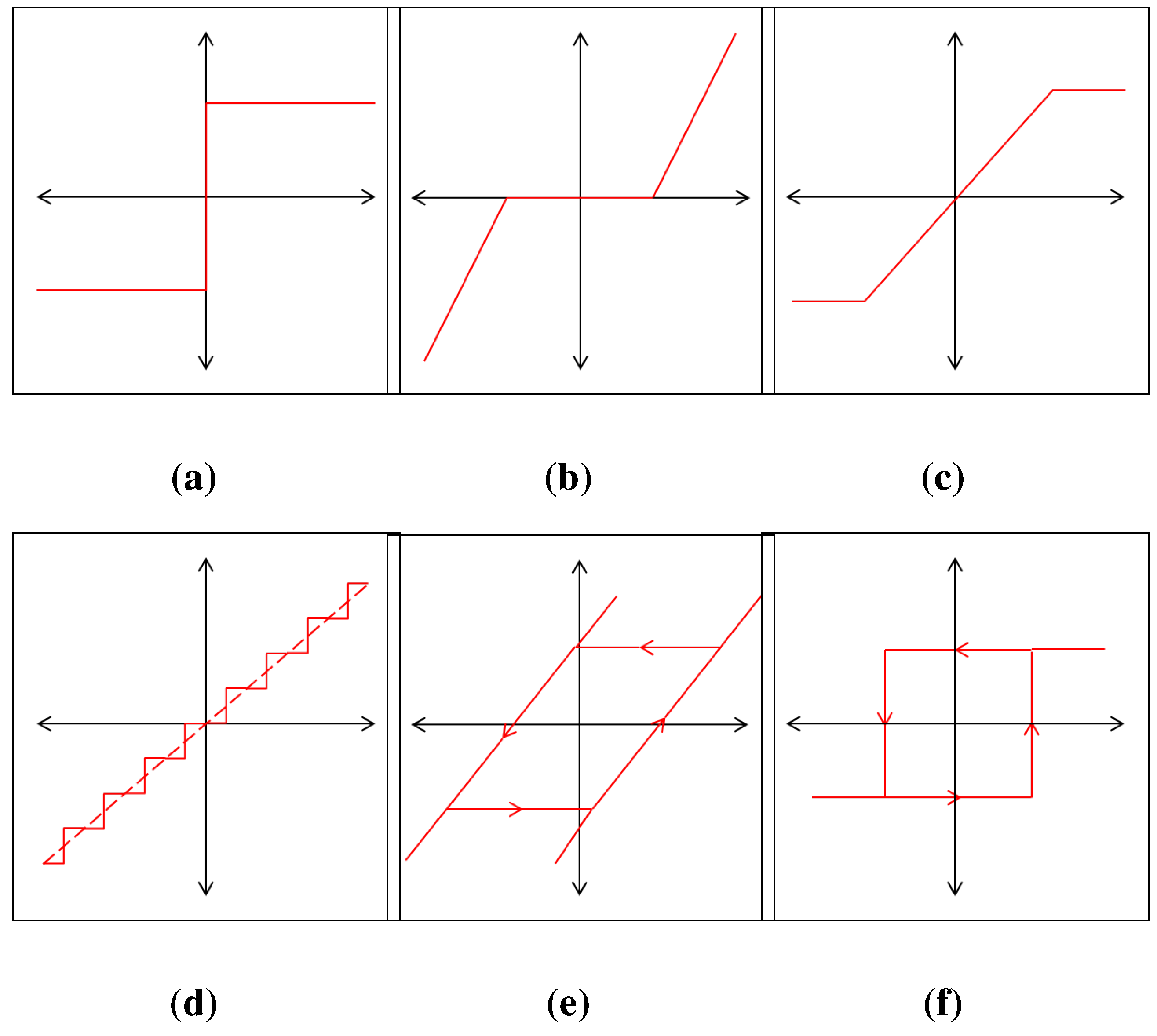
the most) difficult aspects of adaptive control. Unfortunately there cannot be a general nonlinear theory. We must settle for using specific tools and methods that apply to the sets of system structures that we do understand. There are many types of nonlinear behaviors: limit cycles, bifurcations, chaos, deadzone, saturation, backlash, hysteresis, nonlinear friction, stiction,
etc.
Figure 22 shows some example plots of common nonlinearities.
Nonlinear behaviors are sometimes divided into two classes: ‘hard’ and ‘soft’. Soft nonlinearities are those which may be linearly approximated, such as or special types of hysteresis. Typically this means that as long as we do not stray too far from our operating point, we may use linear control methods since we can linearize the system. Hard nonlinearities are those which may not be linearly approximated, such as: Coulomb friction, saturation, deadzones, backlash, and most forms of hysteresis. Hard nonlinearities may easily lead to instability and/or limit cycles, and they unfortunately appear in many real systems. Moreover, since we cannot linearize we are forced to use nonlinear control methods in addition to adaptation. Fortunately for us there are methods for handling nonlinear control design: Feedback Linearization and Backstepping.
Figure 22.
Examples of non-lipschitz nonlinearities. (a) Relay; (b) Deadzone; (c) Saturation; (d) Quantization; (e) Backlash; (f) Hysteresis-Relay.
Figure 22.
Examples of non-lipschitz nonlinearities. (a) Relay; (b) Deadzone; (c) Saturation; (d) Quantization; (e) Backlash; (f) Hysteresis-Relay.
Feedback Linearization is a method in which a nonlinear coordinate transformation between the input and output is found such that the transformed system is linear along all trajectories. The first r-derivatives of the output are the coordinate transformations, and the coordinate transformation is required to be a diffeomorphism (invertible and smooth). We then design the input such that the
output derivative is equivalent to some desired dynamics,
ν, and all nonlinearities are canceled. Consider the following example of system and output dynamics [
93]:
For input-output linearization we essentially take derivatives of
y until the control input shows up in our equations
Our goal is to replace the
with some desired dynamics
ν, so we choose our control input to be
This transforms the system dynamics into
where
and
is some nonlinear coordinate transformation. In order to form a nonlinear coordinate transformation, we need to find a global diffeomorphism for the system in consideration. We know that the Lie derivative is defined on all manifolds, and the inverse function theorem will allow us to form a transformation using the output and its
Lie derivatives. We consider the transformations
and
to construct our diffeomorphism for the example system. However, we still do not have enough functions for a coordinate transformation because we only needed to take two derivatives. The remaining transformation is often referred to as the ‘zero dynamics’ or the ‘internal dynamics’ of the system. In order to find a global diffeomorphism, we need to determine the final coordinate transformation
such that the Lie derivative with respect to
g is zero (as in the first two coordinate changes), shown as
We can see that an easy solution is
. Now we check the Jacobian to see if it is regular (no critical points) for all
x with
The Jacobian is regular for all x and invertible, thus it is a global diffeomorphism. The last step one would normally take is to try and determine whether the zero dynamics are stable or not through functional analysis methods. However, we should beware of the complications that arise when we require all nonlinearities to be canceled. This means that we need to know our system exactly in order to truly have linear dynamics; any unmodeled dynamics can have disastrous effects. The other downside to this method is that the control signal may be unnecessarily large because we also cancel helpful nonlinearities (like ) in the process. It seems as though Feedback Linearization will perform well on systems containing soft nonlinearities, but maybe not on systems with hard nonlinearities unless we use neural networks.
Backstepping was created shortly after Feedback Linearization to address some of the aforementioned issues. It is often called a ‘Lyapunov-Synthesis’ method, because it recursively uses Lyapunov’s second method to design virtual inputs all the way back to the original control input. The approach removes the restrictions of having to know the system exactly and remove all nonlinearities because we use Lyapunov’s method at each step to guarantee stability. Backstepping is typically applied to systems of the triangular form:
We view each state equation in this structure as its own subsystem, where the term coupled to the next state equation is viewed as a virtual control signal. An ideal value for signal is constructed, and the difference between the ideal and actual values is constructed such that the error is exponentially stable by Lyapunov. We may the error of the system to be the state or the difference between the system and a model in the cases of regulation and model following respectively. Assuming a model following problem, we consider a Lyapunov candidate for the first subsystem
Following Lyapunov’s method, we would take the derivative which results in
The
term that connects the first subsystem to the next, is treated as the virtual control input. We choose
as the ideal value for virtual control
such that
becomes
. We will be able to prove that the term containing
is negative definite (guaranteeing stability), but we will be left with an
from substituting in
. This leads us to design a virtual control for the next subsystem in the same fashion, and then combining the Lyapunov candidates to get
This continues on with
as the ideal value for
and their corresponding errors, until we reach the real control input
u. The final Lyapunov candidate function is
One of the main advantages to Backstepping is that we may leave helpful nonlinear terms in the equations. In Feedback Linearization, we have to cancel out all of the nonlinearities using the control input and various integrators. This makes Backstepping much more robust than Feedback Linearization, and also allows us to use nonlinear damping for control augmentation as well as extended matching for adaptation with tuning functions [
53].
5.2. Observability
First consider the LTI system:
For observability, we want to see if we find the initial conditions based on our outputs which is represented by
where
O is the observability matrix we are solving for, and
T is the lower triangular matrix
The observability matrix for this system is then
The observability matrix must be full rank for the system to be fully observable, that is
This is a corollary to saying the system dynamics are injective, or a one-to-one mapping. This states that if the function
f is injective for all
a and
b in its domain, then
implies
. More intuitively, for linear systems this means that if the rows are linearly independent, each state is observable through linear combinations of the output. We can also notice that we can get each column vector in
O by taking the first
derivatives of the output
y. So in order to extend this to nonlinear systems, we can just use the Lie derivative. For nonlinear systems, the observation space
is defined as the space of all repeated Lie derivatives of the covector
, written as
The system is said to be observable if
We can see that this is true if we substitute for , and for . The collection of Lie derivatives will then produce the observability matrix for the LTI system. Finally, an often over-looked but very important part of observability is to check the condition number for the observability matrix of the actual system once sensors and their locations have been chosen. The condition number of the observability matrix can give an indication of how well the sensor choices and locations are for the system at hand. It may also be possible to optimize this process through the use of LMIs. This is especially important for adaptive systems considering their nonlinear behavior, which requires reliable observations to facilitate the adaptation process as well as provide good feedback for the controller.
5.3. Controllability
Consider the same LTI system dynamics
The reachable subspace for the LTI system by the Cayley-Hamilton theorem is
Expanding out the matrix exponential we get the controllability matrix
As with the observability matrix we say the system is controllable if this matrix is full rank, shown as
This is a corollary to saying the system dynamics are surjective, a mapping that is onto. The function f is said to be surjective if for every y in its range there exists at least one x in its domain such that . For linear systems this implies that the columns are linearly independent. It is also important to note that in linear systems, controllability and observability are related through transposition.
We want to find the controllability or reachability for the nonlinear system, so we look at the reachability equation above. After expanding the matrix exponential, we will get a collection of matrix multiplications of
A and
B. For nonlinear systems, we can multiply vector fields by using the Lie bracket. Thus the controllability matrix is the collection of Lie brackets on the vector fields of the nonlinear triangular system, shown as
Like the observability problem, controllability is obtained if the matrix is full rank, and we can easily check this formulation and see that it even works for linear systems by substituting for and B for . Similarly, checking the condition number of the actual controllability matrix after actuators have been chosen and placed is important. An ill-conditioned matrix indicates that the control authority could be improved, which is important for adaptive systems because of the need for high bandwidth response due to the nonlinear nature of the control law.
5.4. Stability & Robustness
Thus far we have not imposed any conditions on the external signals for stability, convergence, or robustness. In doing this we will explore another difference between the direct and indirect methods, as well as the overall robustness of adaptive controllers to external disturbances and unmodeled dynamics. First consider the problem of finding a set of parameters that best fit a data set. We have the actual and estimated outputs
y and
, the set of inputs
, and the actual and estimated parameters
θ and
.
The goal is to minimize the error
e between the actual and estimated outputs
y and
, which is done by considering the squared error below.
We minimize the squared error by differentiating with respect to the parameter estimates
and then rearrange to solve for these estimates
In order for the estimates to be valid, the matrix
must be full rank (non-singular). Extending this to a recursive estimation, we want to minimize the integral of the squared error
We follow the same approach as before by differentiating with respect to the parameter estimate and equating with zero,
The parameter estimate may then be expressed using
where we once again require a non-singular condition on the matrix
. The inverse term is often redefined as a covariance-like variable, which is shown in the RLS algorithm from the Self-Tuning Regulator section. We see that in order to minimize the integral squared error by obtaining accurate parameter estimates, we need the matrix
to be full rank. This condition is often rewritten as
for some non-zero positive constants
and
, and is called the ‘persistent excitation’ condition. The persistent excitation condition was given in the early 1980s by Boyd and Sastry. In the case of the indirect self-tuning regulator, we designed our controller from the perspective that our recursive estimator will give us the correct estimates. If we do not have a persistently exciting reference signal, then our error will not converge to zero, because our parameter estimates will not converge to their true values. In many cases this may be accomplished by adding various types of dither signals to the overall reference signal that we want to track. This shows the key difference between indirect and direct adaptive control methods. Indirect methods rely on the reference signal(s) to be persistently exciting in order to get parameter error convergence which directly affects the tracking error. Direct methods will still achieve tracking error convergence without a persistently exciting reference signal, but if the signal is PE the parameters will also converge to their true values. It can also be shown that given a persistently exciting reference signal, the system will have exponential convergence rather than asymptotic convergence [
94].
Apart from the mathematical condition itself, signals are often determined to be persistently exciting enough based on the number of fundamental frequencies contained within the signal. From the frequency space perspective signals may be approximated by sums of sines and cosines of these frequencies, and
n frequencies may identify up to
independent parameters. When the input signal is persistently exciting, both simulations and analysis indicate that adaptive control systems have some robustness with respect to non-parametric uncertainties. This makes sense because the parameter estimates will converge to their true values, thus the equivalent control principle is truly satisfied and we get a ‘perfect’ controller. However, when the signals are not persistently exciting, even small uncertainties may lead to severe problems for adaptive controllers. Consider Rohrs’ examples [
95], where the system and model are assumed to be
and
However, the real plant is
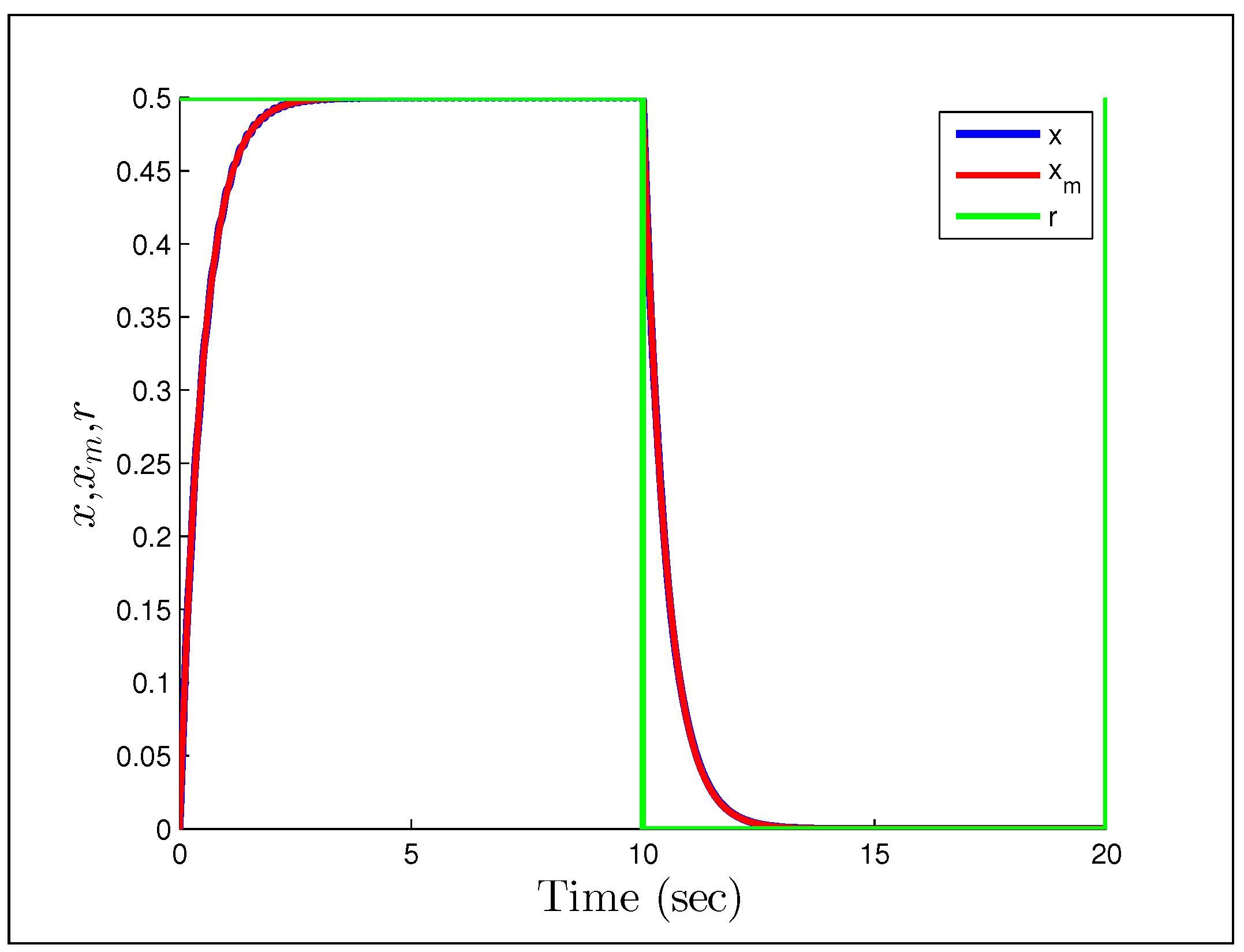
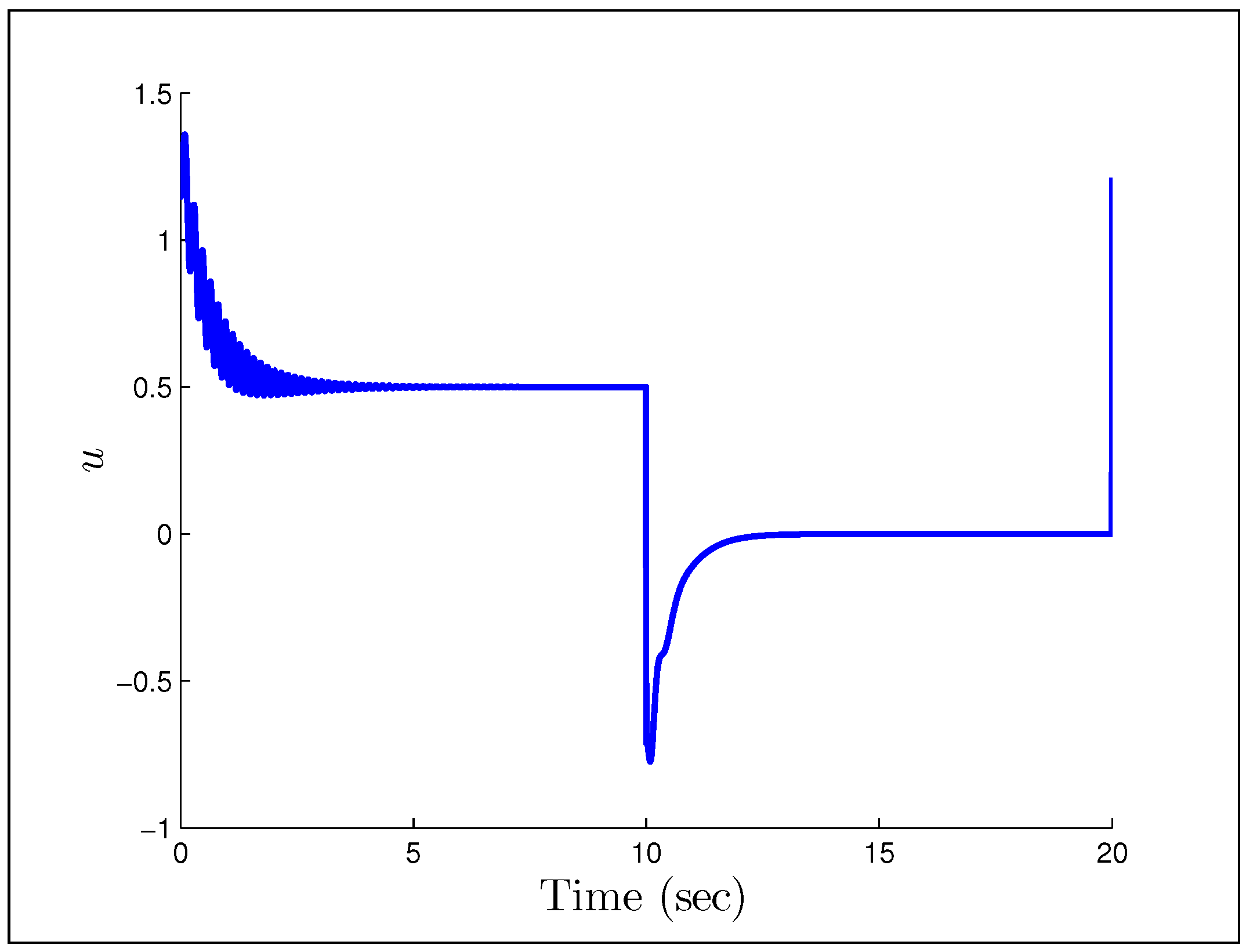
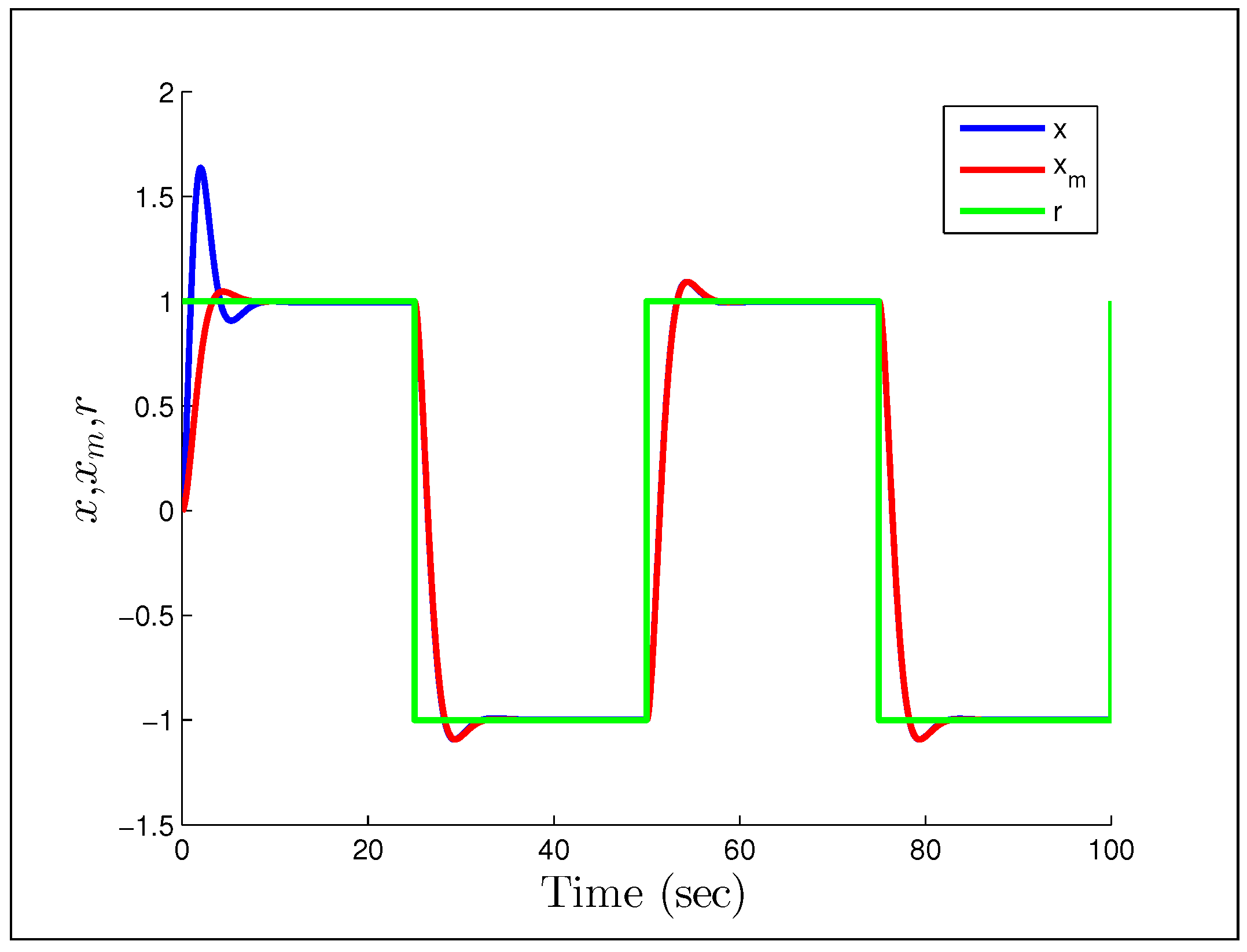
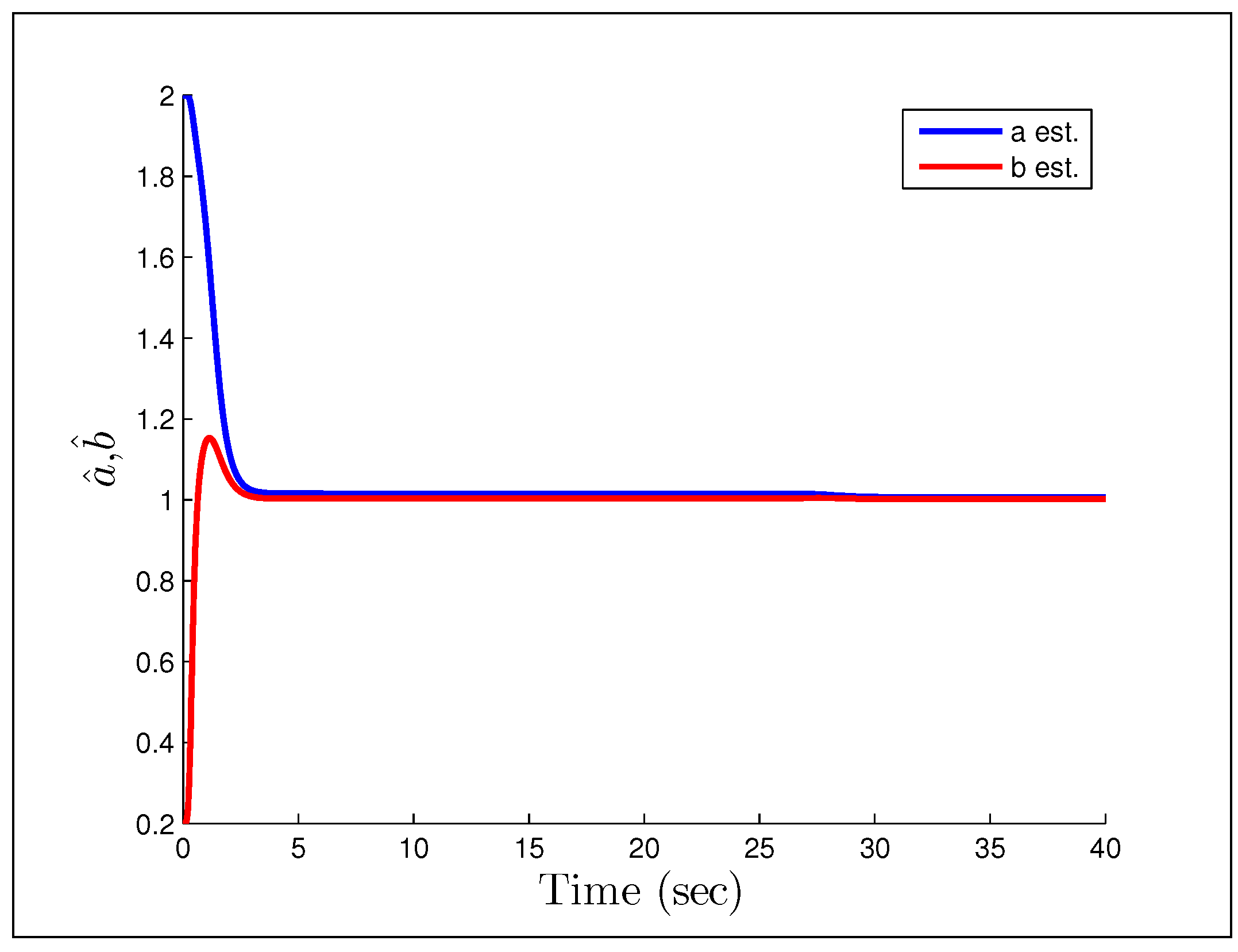
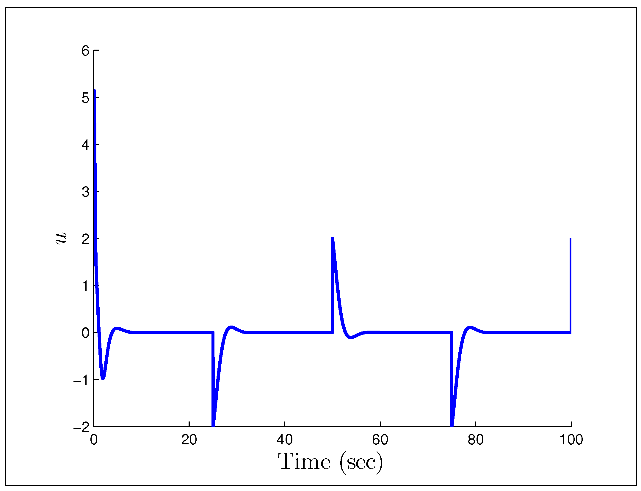
A direct MRAC controller is constructed assuming the plant is of first order, and the initial parameter estimates are and . The first example we look at, is when the reference signal is a constant and the gains we have chosen are .
Figure 23 and
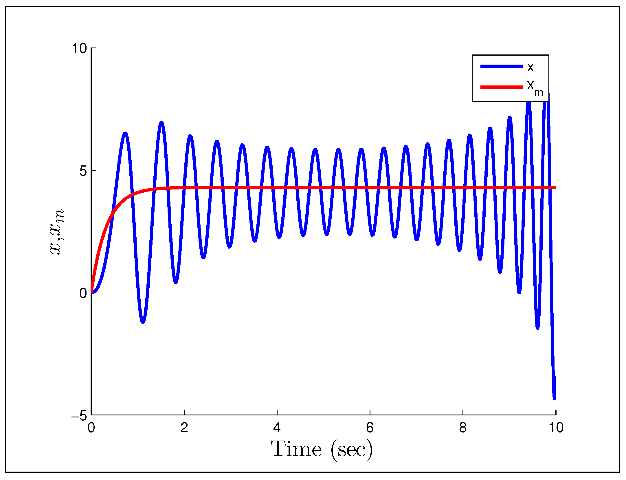
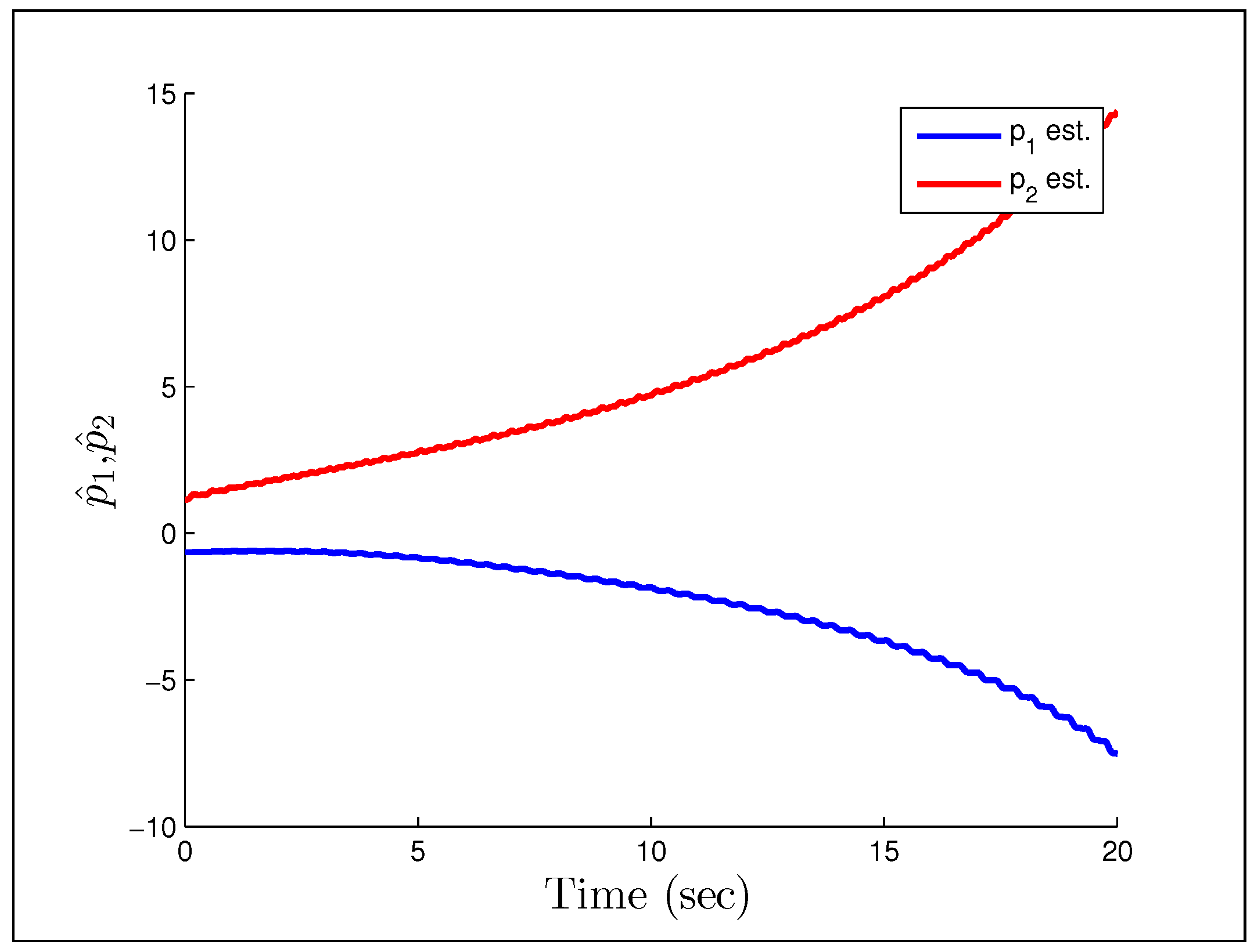
Figure 24 show that having unmodeled dynamics in the system can have disastrous effects even for small adaptation gains. The second example considers the reference signal
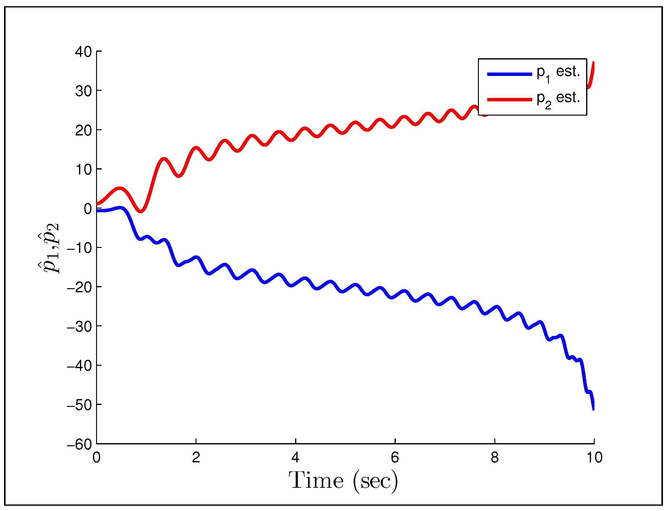
(gains the same), which we would naturally assume to be persistently exciting without the unmodeled dynamics.
Figure 25 and
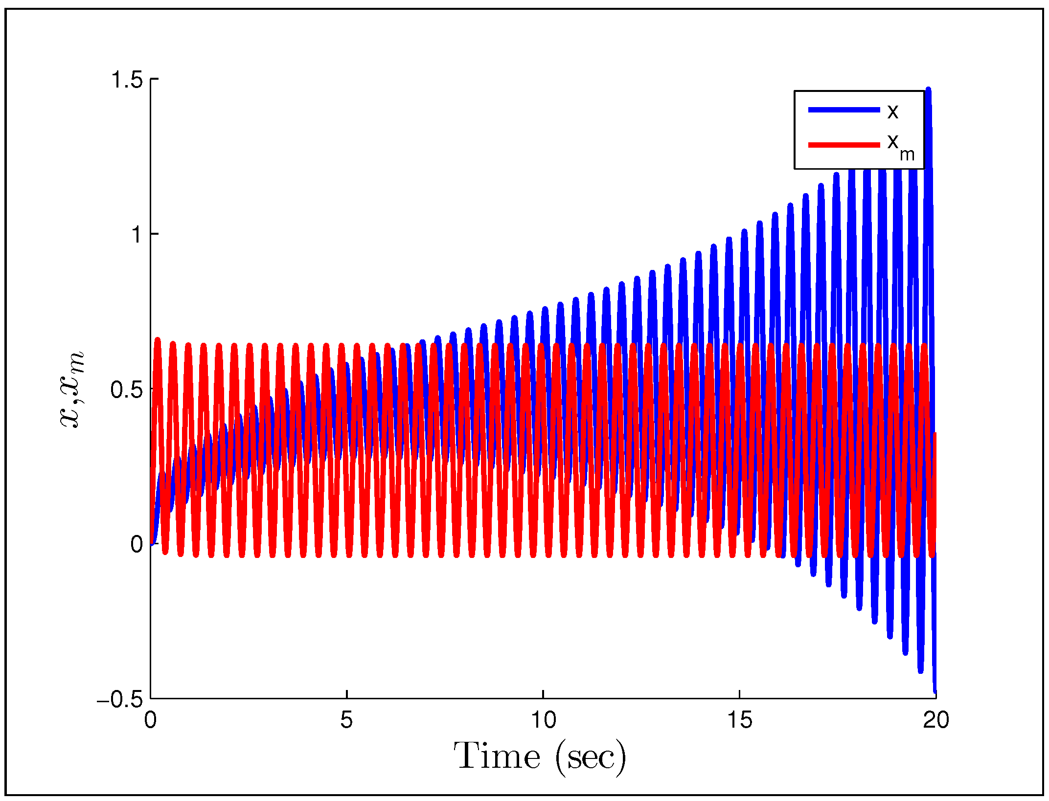
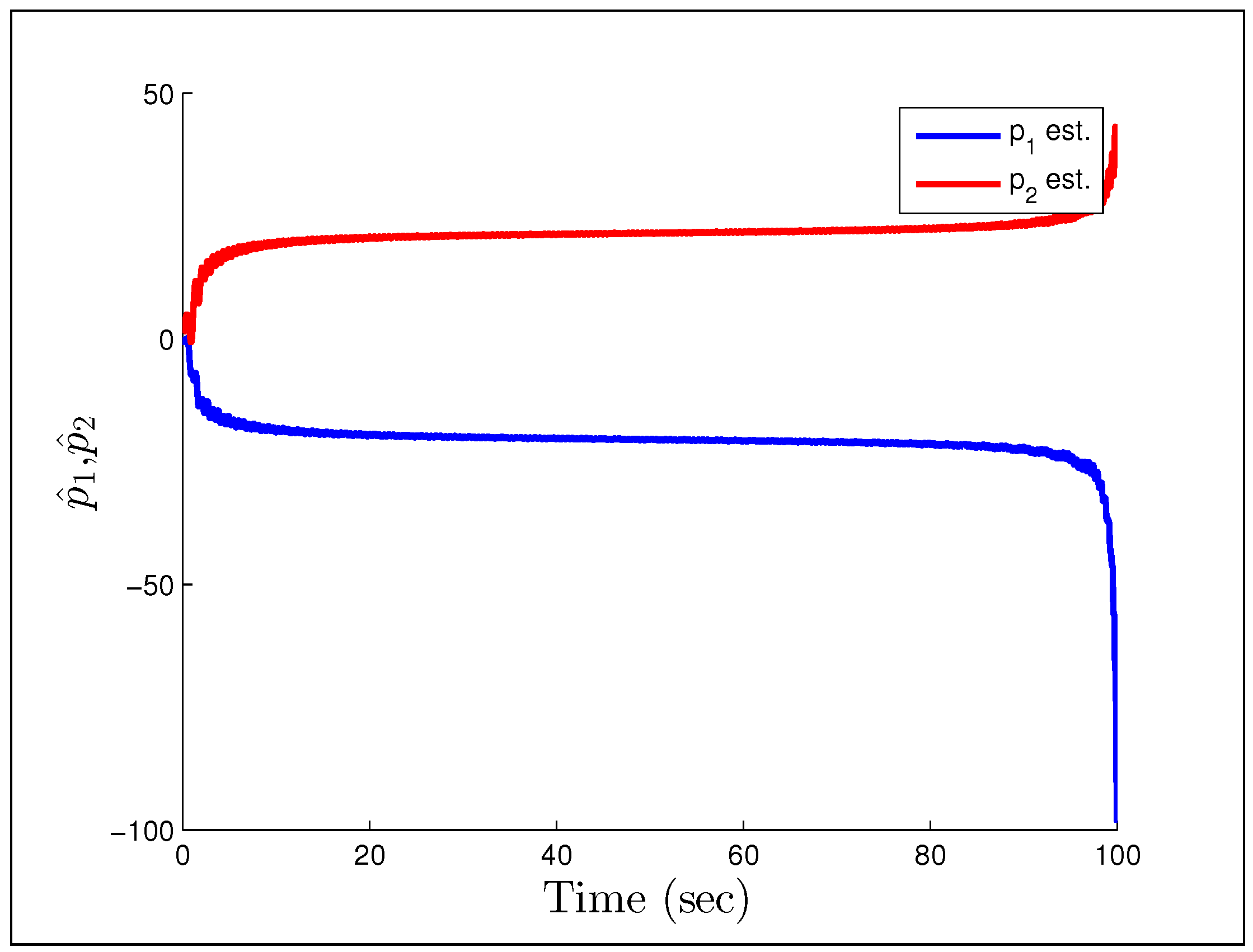
Figure 26 show that the system starts to converge to the constant input, but becomes unstable as the oscillations grow and the parameters drift. The final example considers the case in which we have noise instead of a disturbance, with the reference signal and noise being
and
respectively. We also increase the gains to
.
Figure 27 and
Figure 28 show a particularly troubling result. The system initial converges in both tracking error and parameter estimates, but after some time it becomes wildly unstable and the parameters drift by drastic amounts. Astrom correctly pointed out in a commentary (later added to [
95]) that Rohrs’ examples did not completely characterize the robustness problem, but were never-the-less important to present to the community. While they may not fully characterize the issues, they should successfully motivate the results of the next section.
Figure 23.
Output response for Rohrs’ first example.
Figure 23.
Output response for Rohrs’ first example.
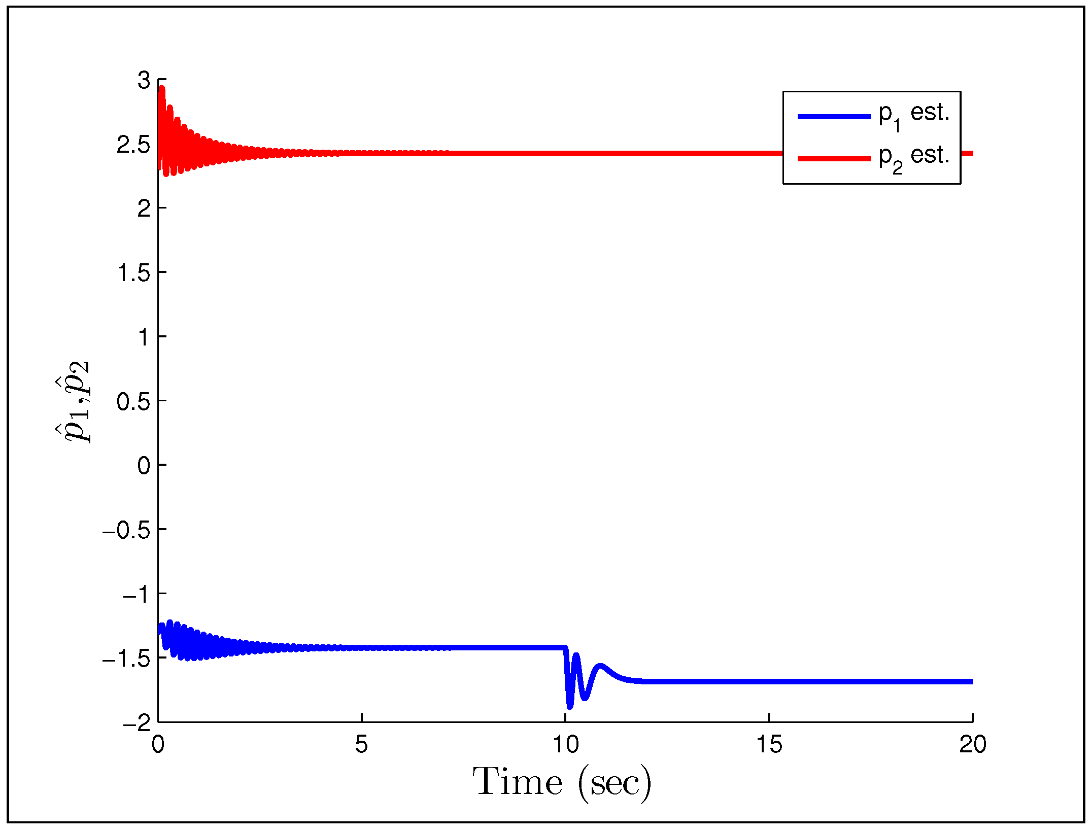
Figure 24.
Parameter estimates for Rohrs’ first example.
Figure 24.
Parameter estimates for Rohrs’ first example.
Figure 25.
Output response for Rohrs’ second example.
Figure 25.
Output response for Rohrs’ second example.
Figure 26.
Parameter estimates for Rohrs’ second example.
Figure 26.
Parameter estimates for Rohrs’ second example.
Figure 27.
Output response for Rohrs’ third example.
Figure 27.
Output response for Rohrs’ third example.
Figure 28.
Parameter estimates for Rohrs’ third example.
Figure 28.
Parameter estimates for Rohrs’ third example.
5.5. Robust Adaptive Control
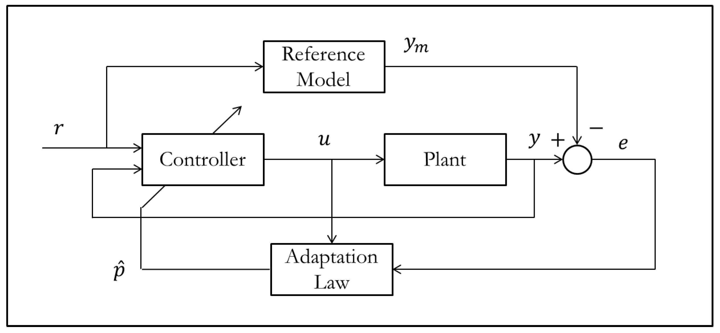
Now that we’ve discussed some of the issues related to adaptation in the presence of noise and disturbances, we present some of the adaptation law modifications that were developed to handle these issues. Control law modifications are mentioned in the next section. First consider the reference model and system with uncertainty:
We construct the control law in the same fashion as MRAC
which gives us the error dynamics that now depend on the uncertainty
We next consider the derivative of the standard quadratic Lyapunov candidate
After plugging in the traditional Lyapunov adaptation law, we may convert this to the following inequality
where
is the bound on the uncertainty. Since we require
to be negative definite the limiting case is when
, and we may solve for the error norm in this case
Anytime the error norm is within this bound,
can become positive and stability may be lost. The parameter error growth will become unstable regardless of the disturbance size, and is known as ‘parameter drift.’ One of the first adaptation law modifications created to handle this problem was the Deadzone method [
21]
which stops adaptation once the tracking error enters the bound establish in the preceding section. While the disturbance issue is solved, not only does the adaptive controller lose its asymptotic error convergence, but the control may chatter as the tracking error hovers around the Deadzone limit. The natural extension to this problem was to try and remove the a-priori bound on the disturbance. The
σ-Modification method [
18] removes the need for an a-priori bound on the disturbance by adding in a correction term as shown below
After plugging this into the derivative of the Lyapunov function we can construct the inequality
which after applying the Holder inequality reduces to
As long as the tracking and parameter errors are outside of these limits the system will remain stable. This method helped to remove the requirement on a-priori disturbance bounds, but presented another problem. If we look at the adaptation law itself, when the tracking error becomes small the trajectory of parameter estimates becomes
and will decay back to the initial estimate. To prevent further modification of the estimates when the tracking error becomes small, the
ϵ-Modification method [
19] replaced the
σ term with the tracking error
The other main drawback for the previous methods is that they can slow down the adaptation, which is the opposite of what we want. The Projection Method [
20] is robust to disturbances and does not slow down the adaptation. Projection does, however, require bounds on the parameter values, but this is often acceptable for real systems. The Discontinuous Projection Algorithm is defined as [
54]
where the projection operator is
The discontinuous projection operator has similar chattering problems to adaptation with a deadzone, which led to the creation of smoothing terms similar to the saturation term in sliding mode control [
22]. Stability analyses for these methods are excluded here to retain some form of brevity, but can be found in their respective references.
5.6. Adaptive Robust Control
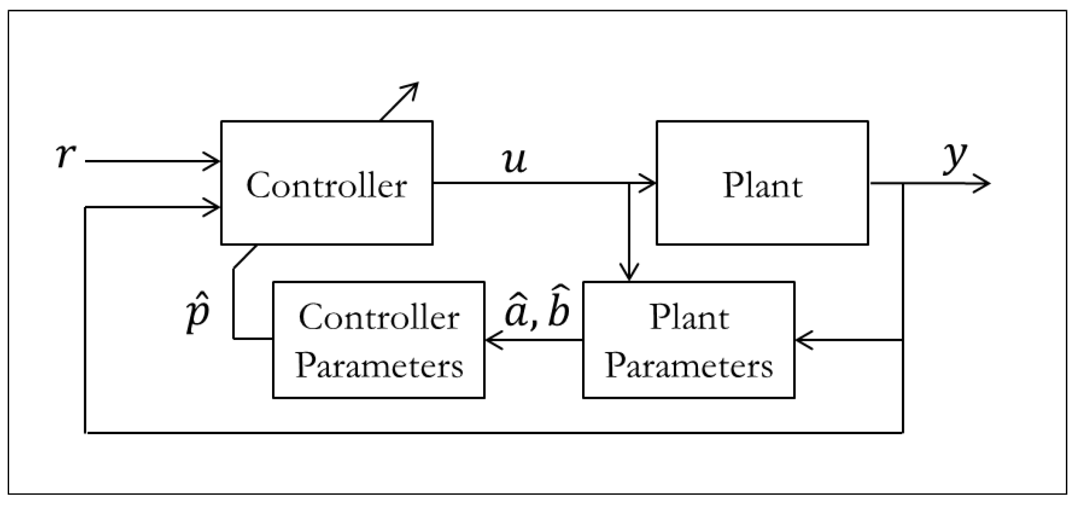
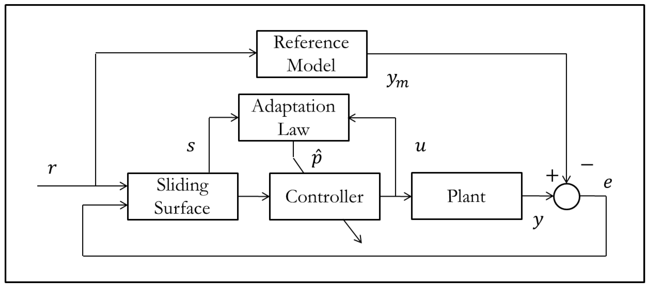
An alternative to just modifying adaptation laws, is to also experiment with various non-equivalent control structures. Yao [
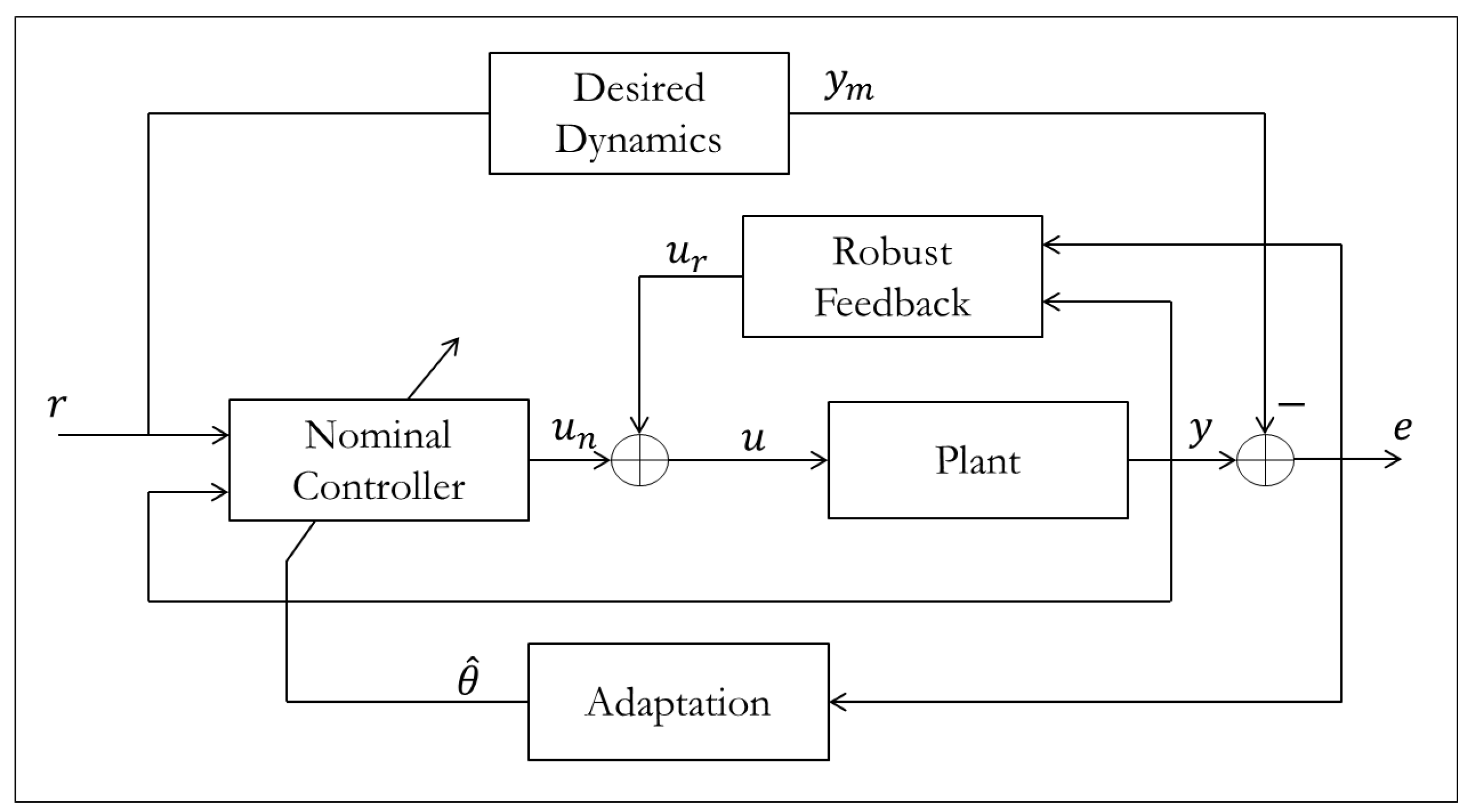
54] approached the robustness problem from this perspective to create the Adaptive Robust Control (ARC) method whose structure is shown in
Figure 29.
Figure 29.
Adaptive robust control structure.
Figure 29.
Adaptive robust control structure.
Assuming that the parameters lie in a compact set and the uncertainty is bounded, we start with a similar system as the previous section (input parameter removed for convenience)
where
. The first input
is the equivalent control input which compensates for the model (
), and the second input
is a robust input. If we define the error as
, we get the error dynamics
We typically separate the robust input into two parts
and
. The first part is typically chosen as
. Thus we get
We want to design the robust input
such that it stabilizes the system with respect to the terms
and Δ. We assume that the components of
are measurable or observable, and we already know that the parameters
θ and uncertainty Δ are bounded. With this information, we may construct a bounding function
that we may use for feedback control such that
An example of a function
that satisfies this inequality is
where the norms of the parameters
θ and regressor
are interpreted component-wise. An example of a robust control law that uses this bounding function is
As before in the sliding mode section, we will want to replace the
term with a smooth function such as
(other options can be found in [
54]). Consider the Lyapunov equation (no adaptation yet)
along with its derivative
Our goal here is to reduce the derivative of the Lyapunov stability equation to
Using the final value theorem we get an error bound for the robust portion of control
and the transient response of the error norm is given by
In order to satisfy the robust tracking error bound as well as its transient, we require the robust portion of the control law to satisfy two requirements
where
ϵ is a positive design parameter. Using the expression for
above (with sgn replaced with sat) the first inequality is obviously true, but the second requirement is not so trivial. When
but we must design
b such that the second requirement is satisfied when
. In this case we get the inequality
If we choose
, then we may rewrite the inequality as
Using the Discontinuous Projection Method for on-line adaptation (
), we may decouple the robust and adaptive control designs, and finally analyze closed loop stability for the overall system. Consider the derivative of the standard quadratic Lyapunov candidate
Plugging in the error dynamics and adaptation law we get
and using the inequalities from the robust control law design we have
It is clear that the first term is negative definite, the second term is negative definite from our robust control law design conditions, and the third term is also negative definite due to the properties of the Discontinuous Projection law. Using this method in conjunction with Backstepping for nonlinear systems makes it extremely powerful especially due to bounded transient performance, but at the expense of a more complicated analysis. The interested reader may refer to [
54] for details and simulations.
6. Perspectives in Control and Adaptation
6.1. Discrete Systems
Adaptive systems are inherently nonlinear, as must be evident by now, and hence their behavior cannot be captured without sufficiently large sampling frequencies. Hence, implementations of adaptation in engineering systems are based on high frequency sampling of system performance and environment, and therefore based on continuous system models and control designs. In those cases where the system is inherently discrete event, e.g., an assembly line, adaptation occurs from batch to batch as in Iterative Learning Control. The most widely used adaptive control is based on a combination of online system identification and Model Predictive Control. This method is ideal for process plants where system dynamics are slow compared to the sampling frequencies, speed of computation, and that of actuation. The actuators in these plants do not have weight or space constraints, and hence are made extremely powerful to handle a wide range of outputs and therefore of uncertainty and transient behavior. In this case a plant performance index such as time of reaction, or operating cost is minimized subject to the constraints of plant state, actuator and sensor constraints, and the discretized dynamics of the plant. Thus, this method explicitly permits incorporation of real world constraints into adaptation. The online system identification is performed using several tiny sinusoidal or square wave perturbations to actuator commands, and measuring resultant changes of performance. It is ideal for the process industry because of the great variability of the physical and chemical properties of feedstock, such as coal, iron ore, or crude oil.
6.2. Machine Learning and Artificial Intelligence
In general there are two types of models: ‘grey box’ and ‘black box’. Black box modeling indicates that hardly anything is known about the system except perhaps the output signal given some input. We have no idea what is inside the black box, but we may be able to figure it out based on the input/output relation. Grey box modeling is a situation where some a-priori information about the system is known and can be used. For example, knowing the design of the system and being able to use Newton’s laws of motions to understand the dominating dynamics would be considered grey box modeling. Even though we may know a lot about the system, there is no way we can know everything about it, hence the ‘grey’ designation. Uncertainty in our models and parameters are fundamental problems that we must unfortunately deal with in the real world.
The presence of uncertainty and modeling difficulties often leads to the field of machine learning, the process of machines ‘learning’ from data. Put simply, we approximate a relationship (function) between data points, and then hopefully achieving correct predictions based on its function approximation if it is to be used in control. There are many methods associated with machine learning (e.g., Neural Networks, Bayesian Networks, etc.), but we should be very careful in how and where we implement these algorithms. There are situations where using machine learning algorithms provide a significant advantage to the user and situations where it would be disadvantageous.
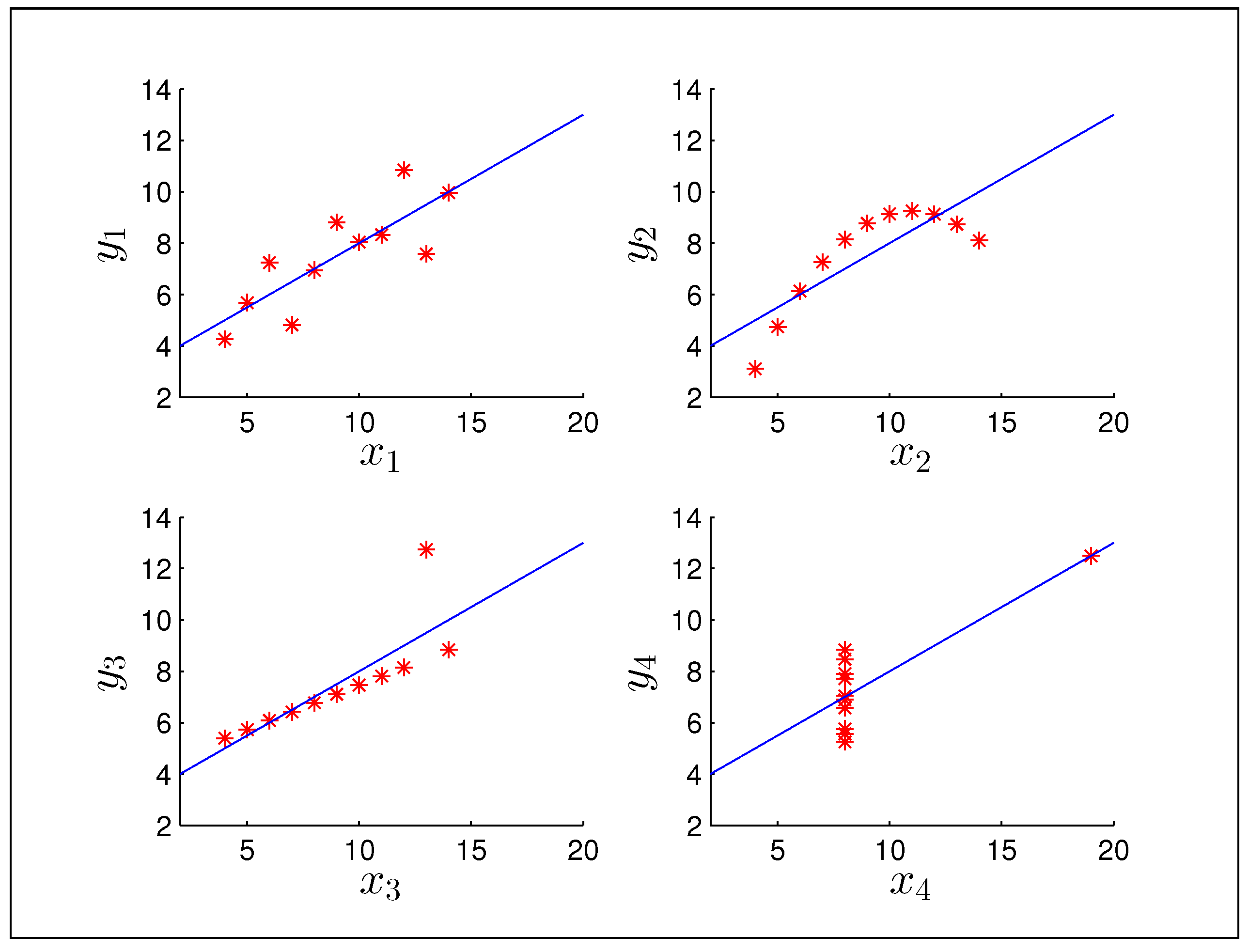
An example of a system where machine learning would be advantageous is a highly articulated robot such as a humanoid robot. A system of this type has too many states to handle in practice, not to mention complexities due to nonlinearities and coupling, so a machine learning algorithm would be very advantageous here. However, since the algorithm can only improve the function approximation by analyzing data, this approach obviously requires a lot of ‘learning’ time as well as computational resources. Therefore the system (or its data) has to be available to be tested in a controlled environment which is not always possible (consider a hypersonic vehicle). The other disadvantage to certain types of machine learning algorithms is illustrated by Anscombe’s Quartet, shown in
Figure 30.
Figure 30.
Anscombe’s quartet.
Figure 30.
Anscombe’s quartet.
Anscombe’s Quartet was a famous data set given by Francis Anscombe [
96] to show the limitations of regression analysis without graphing the data. Each of the significantly different data sets has the exact same mean, variance, correlation, and linear regression line. This shows that there will always be outliers that manipulate the system, but also that we should attempt to have a universal function identifier if we cannot narrow down the distributions of data we will see. There are machine learning algorithms that are universal function identifiers (see the Cybenko Theorem), but these theorems rest on the assumption that design parameters are correctly chosen, which is far from easy. This further illustrates the importance of the ‘learning’ period and training data, as well as using as much a-priori information as possible when it is available. That being said, machine learning algorithms have been successfully applied to a wide variety of very complex problems and constitute a fertile research topic. Some open problems related to Neural Networks are presented later.
6.3. Abstract Viewpoints
The fields of differential topology, differential geometry, and Lie theory are considerably more abstract than many are used to, but may offer a tremendous advantage to visualizing and thinking about more complex spaces. Topology is the study of the properties of a mathematical space under continuous deformations, and its differential counterpart is the study of these with respect to differentiable spaces and functions/vector fields. Differential geometry is quite similar to differential topology, but typically considers cases in which the spaces considered are equipped with metrics that define various local properties such as curvature. Lie theory is the mathematical theory that encompasses Lie algebras and Lie groups. Lie groups are groups that are differential manifolds, and Lie algebras define the structures of these groups. The combination of these fields allows us to classify and perform calculus on these spaces abstractly, regardless of their dimension. An example of the advantage of even understanding some of the most basic concepts is finding the curvature of a higher dimensional space. For problems in 3-dimensional space the cross-product can be used to find curvature, but the cross-product itself is only defined up to this dimension and thus cannot be used for n-dimensional problems. Differential geometry allows one to define curvature in an abstract sense for systems of any order, which will also be equivalent to the cross-product in 3-dimensional problems. We have already used some methods from these fields earlier in this paper, such as finding diffeomorphisms for Feedback Linearization and the Lie bracket for observability/controllability in nonlinear systems. For brevity we did not include the backgrounds of all of these fields, but the interested reader may refer to for more complete treatments of the subjects.
7. Open Problems and Future Work
Despite the extensive decades of research in adaptive control and adaptive systems, there are still many unsolved problems to be addressed. Some of these problems may not be ‘low hanging fruit’; however, their solution could lead to important applications. We discuss a few of these problems in this section. First, we discuss nonlinear regression problems, followed by transient performance issues. Finally qualify developing analysis tools that can ease the proofs of stability and boundedness for complex systems, as well as developing novel paradigms for adaptive control.
7.1. Nonlinear Regression
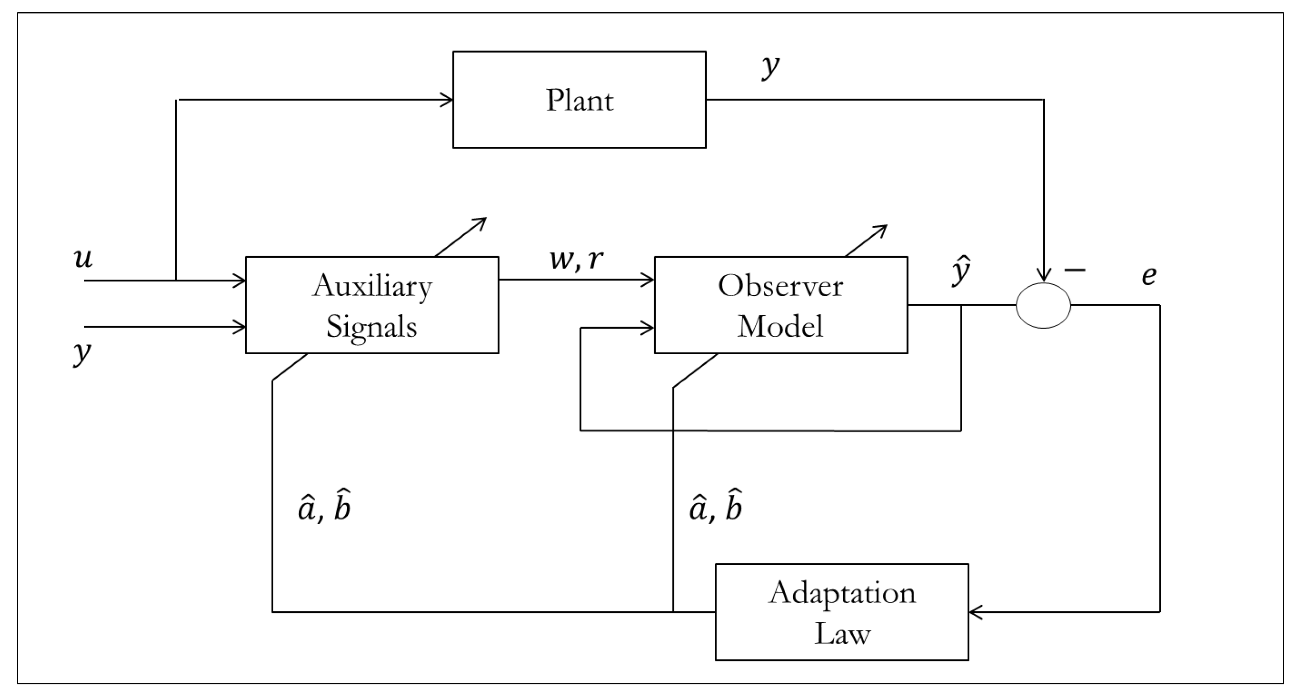
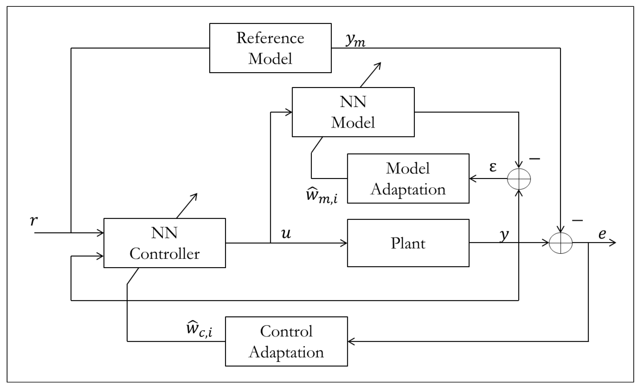
As with systems that are nonlinear in their states, there is no general nonlinear regression approach, it consists of a toolbox of methods that depend on the problem. Parameters appear linearly for many systems, but there are some systems (especially biological) where they appear nonlinearly. This happens to be one of the largest obstacles in the implementation of neural networks. In many neural network configurations, some parameters show up nonlinearly, and are typically chosen to be constant (lack of confidence guarantees), or an MIT rule approach is used (lack of stability guarantees). Even if network input and output weights show up linearly and adaptation laws are chosen using Lyapunov, it is all for naught if the nonlinear parameters are incorrect which can require extensive trial and error tuning by the designer or large amounts of training. An example of how control and identification may be used in an MRAC-like system is given in
Figure 31.
The Radial Basis Function Neural Network design is a good example of when we might encounter difficulties related to nonlinear parameters. A basic RBFNN controller uses Gaussian activation functions that are weighted to form the control input
u as shown in
Figure 31.
Neural networks for MRAC.
Figure 31.
Neural networks for MRAC.
The weights w appear linearly, and if we had ideal values for the centers c and biases b then we could easily construct a Lyapunov function to adapt the weights. However, finding ideal values for c and b can be quite difficult, so it would be advantageous to also find Lyapunov stable update laws for them as well. Logarithmic transformations exist for regression problems of the form , but performing these transformations simultaneously with Lyapunov analysis can become quite overwhelming and even produce further problems related to the parameters that do not appear in the exponent. If more progress is made in finding transformations for turning nonlinear regression problems into linear ones, the field of neural networks and artificial intelligence can grow significantly. Training time for many systems will be significantly reduced, proving Lyapunov stability may become more tractable, and the problem illustrated by Anscombe’s quartet may be reduced.
7.2. Transient Performance
Adaptive controllers have the advantage that the error will converge to zero asymptotically, but for controlling real systems we often care more about the transient performance of the controlled system. It is generally not possible to give an a-priori transient performance bound for an adaptive controller because of the adaptation itself. When we use Lyapunov’s second method to derive an adaptation law, we are guaranteeing error convergence at the expense of parameter error convergence. Higher adaptation gains typically lead to faster convergence rates, but this is not always true given the instabilities that arise from high adaptation gains. Consider the standard scalar Lyapunov function
After the adaptation law is chosen
(assuming no disturbances or modeling uncertainty). Setting up an inequality we may say that
. Now let’s analyze the
norm
The main problem here is that we do not have a good idea what the initial parameter errors are, so it is difficult to give a-priori predictions of transient performance. There are four common ways to help improve the transient performance: increase , increase , use correct trajectory initialization to minimize , and perform system identification to minimize and . Increasing is obviously a good way to improve performance, but this may not be an option depending on the control authority in the system (e.g., bandwidth, power, etc.). Increasing is an option for ideal systems but as we discovered before, high adaptation gains in real systems can lead to instability and this will depend on the specific system at hand.
The use of robust adaptive control methods helps mitigate the stability problem, but at the expense of slowed transient performance or convergence to an error bound rather than zero. The projection method is reported to maintain fast adaptation and stability, but requires the designer to have bounds on parameters. This is not an unreasonable assumption, but there may be cases where it does not apply. Carefully initializing the trajectory to set is an option that can be applied to most systems and does not pose any additional problems. Lastly, good system identification can provide accurate parameter estimates to initialize with in order to minimize and , but this also assumes that the system may easily/cheaply be identified and that the correct identification method is used. There are many systems in existence that have highly nonlinear parametric models that are difficult (or impossible) to accurately identify with existing methods, or may be too costly to identify frequently. Improving transient performance is an on-going research problem in adaptive systems.
7.3. Developing Analysis Tools
The complexity of the tools needed to analyze the stability of a system grows with the complexity of the system. In this context, system has a broad meaning and is defined as a set of ordinary or partial differential equations. With this point of view, a control problem also reduces to a stability problem. For example, a control problem in which the objective is the perfect tracking of state variables, turns into a stability problem when we define tracking error and look at the governing error dynamics as our “system”. The stability of systems have been widely studied for more than a century, from the work of Lyapunov in 1900s. Hence, we will not discuss those results; however, we will mention a few areas where improvements could be made. The benefit of such research is twofold. Any new tool developed will have applications to any branch of science that deals with “dynamics”, i.e., any system that changes with time.
In order to provide more motivation, consider the following scenario. We have derived an adaptive control law for a nonlinear non-autonomous system under external disturbances. We would like to prove that the state tracking error converges to zero despite disturbances and the parameter tracking errors are at least bounded. If we fail this task, we would like to at least prove that the states remain bounded under disturbances, and that the error remains within a finite bound the whole time.
Non-autonomous systems are explicitly time-dependent and are generally described as
where
is a function over some domain
. Simply put, a non-autonomous system is not invariant to shifts in the time origin. That is, changing
t to
will change the right hand side of the differential equation. The stability of such systems is most commonly studied via one of the following two approaches: (1) averaging theorems and (2) non-autonomous Lyapunov theorems.
7.3.1. Averaging Theorems
The first method is known as the averaging method, and applies to systems of the form
where
ε is a small number. Note that any system of form Equation (
205) can be transformed to Equation (
206) by the transformation
. General averaging theorems only require that
f be bounded at all times on a certain domain. However, a simpler class of averaging theorems further require that
f be
T-periodic in
t. The idea of averaging method is to integrate the system over one period. This process yields the average system as
where
. This removes the explicit time dependence and enables the use of vast stability theorems applicable to autonomous systems. However, the main question is whether the response of the new system is the same as the original system. The following theorem from [
90] addresses this issue.
Theorem 1 ([
90]).
Let and its partial derivatives with respect to up to the second order be continuous and bounded for ,
for every compact set ,
where is a domain. Suppose f is T-periodic in t for some and ε is a positive parameter. Let and denote the solutions of (206) and (207), respectively. If and ,
then there exists such that for all ,
is defined and If the origin is an exponentially stable equilibrium point of the average system Equation (207),
is a compact subset of its region of attraction,
,
and ,
then there exists such that for all ,
is defined and If the origin is an exponentially stable equilibrium point of the average system, then there exists positive constants and k such that, for all ,
Equation (206) has a unique, exponentially stable, T-periodic solution with the property .
Now suppose we want to apply this theorem to our hypothetical scenario and prove the stability of our adaptive controller. A reader familiar with adaptive control already knows that unless PE conditions are satisfied, the stability is only asymptotic. This means that parts 2 and 3 of this theorem will not be applicable, leaving us only with part 1. However, this part is also a weak result which is only valid for finite times. Therefore, averaging theorem in this form is not helpful in proving stability of adaptive control applied to non-autonomous systems.
Teel
et al. [
97,
98] have shown that if the origin of the system is asymptotically stable with some additional conditions, then we can deduce practical asymptotic stability of the actual system. However, their theorem cannot be used in this scenario either. This is due to the fact that when we have asymptotic stability in adaptive control, the parameter errors generally do not converge to the origin. So even though the state tracking error converges to the origin, the parameters in general will converge to an unknown equilibrium manifold. This is sometimes referred to as “partial stability” and we will discuss it further. Therefore, one area of improving tools is to devise averaging theorems that not only work for asymptotically stable system, but also account for systems with partial stability where only state errors converge to the origin.
7.3.2. Non-Autonomous Lyapunov Stability
In search for a proper tool to analyze our hypothetical scenario, we next move on to Lyapunov theorems for non-autonomous systems. Such theorems, directly deal with systems that are explicitly time-dependent and are much less developed than theorems regarding autonomous systems. Khalil [
90], Chapter 4, provides three such theorems one of which is mentioned here.
Theorem 2 ([
90]).
Let be an equilibrium point for Equation (205) and be a domain containing .
Let be a continuously differentiable function such that and ,
where ,
,
,
and a are positive constants. Then,
is exponentially stable. If the assumptions hold globally, then is globally exponentially stable.
In adaptive control, it is extremely difficult to satisfy condition (211). The derivative of the Lyapunov function is usually only semi-negative definite at best. This means that the right hand side of Equation (211) will only have some of the states and the inequality will not hold. We believe that creating new Lyapunov tools with less restricting conditions is an area that needs more attention.
7.3.3. Boundedness Theorems
When we cannot study the stability of the origin using known tools, or when we do not expect convergence to the origin due to the disturbances, the least we hope for is that
x will be bounded in a small region. Boundedness theorems consider such cases and several of them are addressed in Chapter 9 of [
90] who categorizes perturbations into vanishing perturbations and non-vanishing perturbations. The general approach is to separate the perturbation terms from the system. Therefore, the system is described as
where
is the perturbation term, and
is a domain that contains the origin
. Note that the perturbation term could result from modeling errors, disturbances, uncertainties,
etc. Therefore, boundedness theorems have wide applications in realistic problems.
Vanishing perturbations refer to the case where . Therefore, if is an equilibrium of the nominal system , then it also becomes an equilibrium point of the perturbed system. Non-vanishing perturbations refer to cases where we cannot determine whether . Therefore, the origin may not be an equilibrium point of the perturbed system.
Such theorems, although very useful in many cases, still need further development before they can be applied to our scenario and be useful for adaptive control. Most boundedness theorems require exponential stability at the origin. We know that in adaptive control, exponential stability is only possible when PE conditions are satisfied (in which case our first approach to use averaging theorems would have worked already!). Furthermore, in the absence of PE, the origin is not a unique equilibrium for the adaptive controller: some parameter estimates may converge to an unknown equilibrium manifold and we cannot transform the equilibrium of the adaptive controller to the origin. Since the objective of the adaptive controller is not the identification of parameters, but rather the convergence of tracking error, one wonders whether it is possible to study the stability of only parts of the states (i.e., the stability of the state tracking error). This is sometimes referred to as partial stability.
7.3.4. Partial Stability and Control
The first person to ever formulate partial stability was Lyapunov himself – the founder of modern stability theory. During the cold war, with the resurgence of interest in stability theories, this problem was pursued and Rumyantsev [
99,
100] published the first results. Much research has been done on partial stability all over the world, but mostly in Russia and the former USSR. For example, see [
101,
102,
103,
104,
105,
106]. Since this topic might be unfamiliar to many readers, we explain it a little further and refer the enthusiastic reader to the papers cited. In particular [
103] provides a comprehensive survey of problems in partial stability.
Partial stability deals with systems for which the origin is an equilibrium point, however, only some of the states approach the origin. Such systems commonly occur in practice, and there have been a fair amount of research on their stability analysis using invariant sets and Lyapunov-like lemmas such as Barbalat’s Lemma or LaSalle’s Principle. Some of the motives for studying partial stability are [
103]: systems with superfluous variables, sufficiency of partial stability for normal operations of system, estimation of system performance in “emergency” situations where regular stability is impossible, and the difficulties in rigorous proofs of global stability.
The problem of partial stability is formulated as follows. Consider the system
where
is piecewise continuous in
t, locally Lipschitz in
x on
, and
contains the origin
. We break the state space into two sets of variables by writing
where
y represents the variables converging to the origin, and
z represents that variables that may or may not converge to origin. Thus, we write Equation (
213) as
We say
is an equilibrium point for Equation (
213), if and only if
. This translates to
. Partial stability is defined as follows
Definition 1. An equilibrium point of Equation (215) isy-
stable, if for any ,
and ,
there exists a such that uniformly y-stable, if it is y-stable, and for each ε, is independent of .
asymptotically y-stable, if it is y-stable, and for any , there exists a positive constant such that every solution of Equation (215) for which , satisfies as .
uniformly asymptotically y-stable, if it is uniformly y-stable, and there is a positive constant c, independent of ,
such that for all ,
as ,
uniformly in t. Meaning that for each ,
there exists such that
There’s a myriad of theorems regarding partial stability of systems. However, in most these works, the conditions on the Lyapunov function are too restrictive, rendering them ineffective for the adaptive control problem of our interest. Furthermore, the behavior of systems under perturbations is not abundantly studied when the best we can do is partial stability. However, we believe that adaptive control could in general benefit from this tool due to the nature of its stability. Further development of partial stability tools and its application to adaptive control is an interesting problem that can be addressed.
7.4. Underactuated Systems
Systems that have fewer actuators than states to be controlled are referred to as underactuated. These systems are of interest from several viewpoints. First, in some applications it may not be possible to have actuators for all the desired states. Secondly, if an actuator failure happens the system descends into an underactuated mode. A successful control design for such situations can greatly enhance the safety and performance of the systems. Thirdly, a deliberate reduction in the number of actuators and reduce the manufacturing costs.
Underactuated systems have been studied for more than two decades now. Energy and passivity based control [
107,
108,
109], energy shaping [
110], and Controlled Lagrangians and Hamiltonians [
111,
112,
113,
114,
115,
116] are just a few methods among others proposed [
117,
118,
119,
120].
A survey on the methods and problems of underactuated systems requires a separate full length paper. However, we only look at them from the adaptive control perspective. Most of these proposed methods do not deal with uncertainties. Very few papers have been published that address the uncertainty issue in underactuated systems [
121]. Addition of adaptation and adaptive control laws to methods that deal with underactuated systems is a subject that has been left mostly untouched. Research in these areas can greatly enhance the toolbox that we currently have for dealing with uncertain systems.
7.5. Possible New Methods
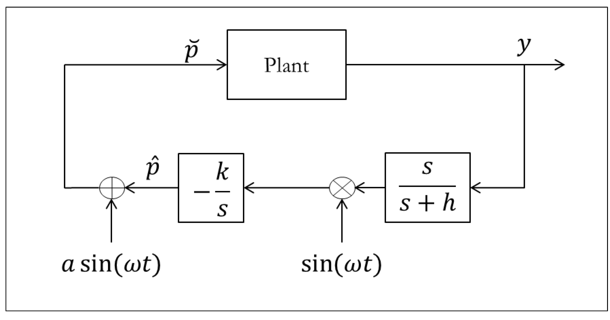
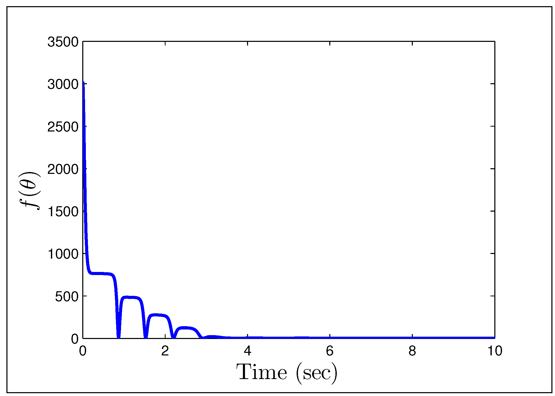
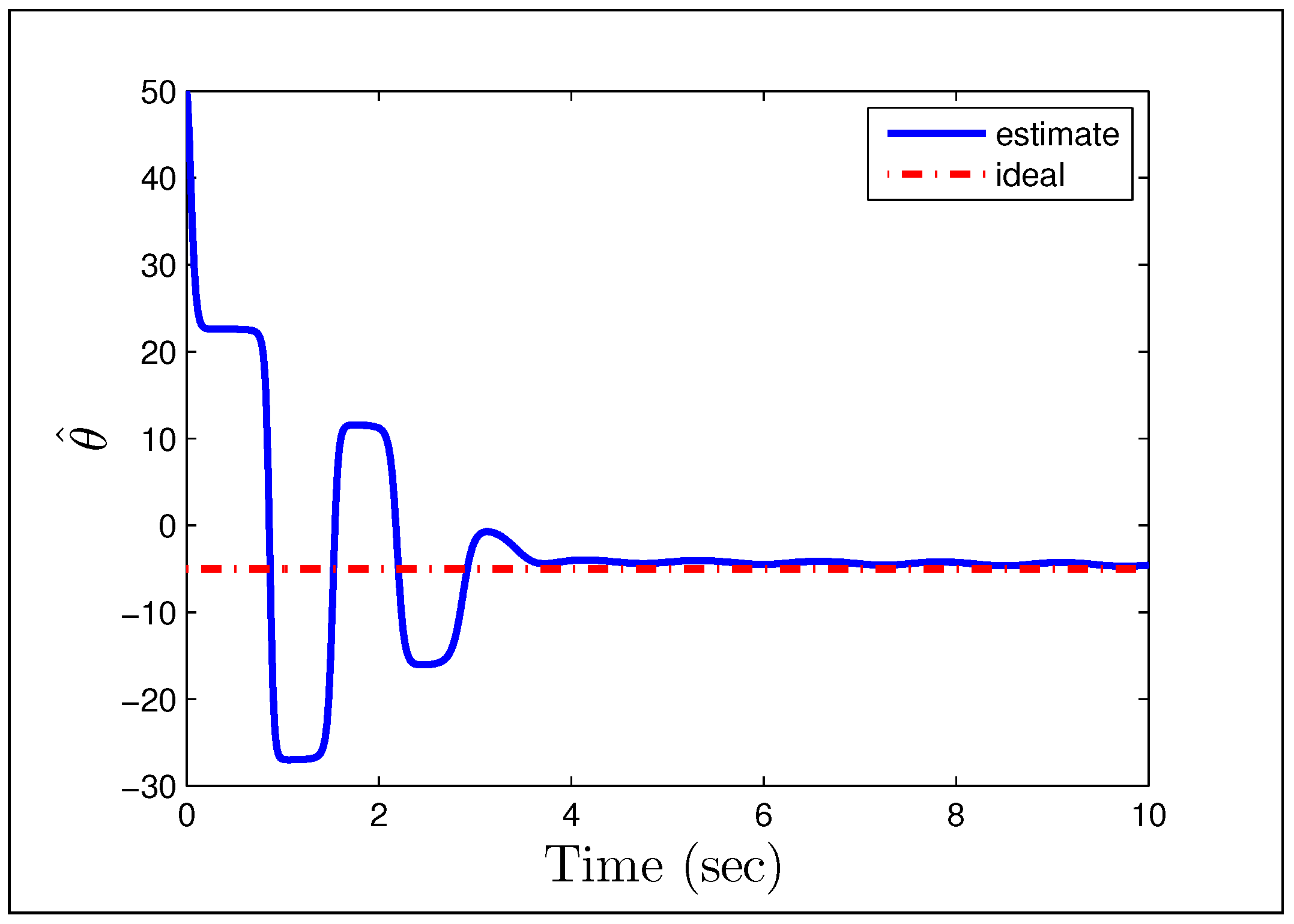
Although very difficult, it is still possible to create novel paradigms for adaptive control. Recently, [
122,
123,
124,
125] attempted at a new paradigm of adaptive control by employing Extremum Seeking as a means of adaptation (rather than a means of optimization). Their method augments the Model Reference Adaptive Controller with an adaptation law using Extremum Seeking loops. The main difference between this approach and the mainstream adaptive methods is that the adaptation occurs in real-time and no mathematical adaptive laws need be derived. This makes the implementation simple; however, it also brings several downsides that have not been addressed. Extremum Seeking perturbs the system. Therefore, the system requires some inherent robustness to perturbations, or if this is not the case, the controller must provide such robustness. Due to the addition of deliberate perturbations to the system, one expects that PE conditions would be automatically satisfied, making the real-time identification of parameters possible. However, this does not seem to be the case. Further study needs to be done, before this new paradigm becomes an acceptable method.

