1. Introduction
Emergence has been characterized as taking place in strong and week forms. Mittal [
1] pointed out that strong emergent behavior results in generation of new knowledge about the system representing previously unperceived complex interactions. This can occur in the form of one or more of new abstraction levels and linguistic descriptions, new hierarchical structures and couplings, new component behaviors, and new feedback loops. Once understood and curated, the behavior returns to the weak form, as it is no longer intriguing, and then can begin to be treated in regularized fashion. Emergent behavior is likely an inherent feature of any complex system model because abstracting a continuous real-world system (e.g., any complex natural system) to a constructed system-model must leave gaps of representation that may diverge in unanticipated directions. In [
2] philosophically, following Ashby [
3] and Foo and Zeigler [
4], the perceived global behavior (holism) of a model might be characterized as: Components (reductionism) + interactions (computation) + higher-order effects where the latter can be considered as the source of emergent behaviors [
5,
6].
The Discrete Event Systems Specification (DEVS) formalism has been advocated as an advantageous vehicle for researching such structure–behavior relationships because it provides the components and couplings for models of complex systems and supports dynamic structure for genuine adaption and evolution. Furthermore, DEVS enables fundamental emergence modeling because it operationalizes the closure-under-coupling conditions that form the basis of well-defined resultants of system composition especially where feedback coupling prevails [
7,
8].
In this paper, we formulate conditions under which a composition of component systems form a well-defined system-of-systems at a fundamental level. Formal statement of what defines a well-defined composition and sufficient conditions guaranteeing such a result offer insight into exemplars that can be found in special cases such as differential equation and discrete event systems. Informally stated, we show that for any given global state of a composition, two requirements can be stated as: (1) the system can leave this state, i.e., there is at least one trajectory defined that starts from the state; and (2) the trajectory evolves over time without getting stuck at a point in time. Considered for every global state, these conditions determine whether the resultant is a well-defined system and if so, whether it is non-deterministic or deterministic. We formulate these questions within the framework of iterative specifications for mathematical system models that are shown to be behaviorally equivalent to the Discrete Event System Specification (DEVS) formalism. This formalization supports definitions and proofs of the afore-mentioned conditions and allows us to exhibit examples and counter-examples of condition satisfaction. Drawing on Turing machine halting decidability, we investigate the probability of legitimacy for randomly constructed DEVS models. We close with implications for further research on the emergence of new classes of well-defined systems.
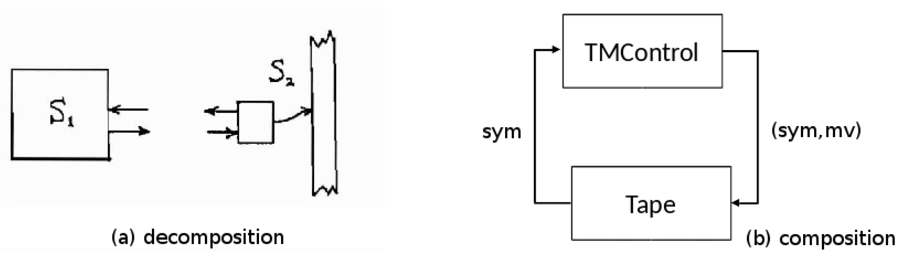
Let us start with a well-known concept, the Turing Machine (TM) (cf. [
9]). Usually, it is presented in a holistic, unitary manner but as shown in
Figure 1b, we can decompose it into two stand-alone independent systems: the TM Control (
) and the Tape System, (
). Foo and Zeigler [
4] argued that the re-composition of the two parts was an easily understood example of emergence wherein each standalone system has very limited power but their composition has universal computation capabilities. Examining this in more depth, the Tape system shown in
Figure 1a is the dumber of the two, serving a memory with a slave mentality, it gets a symbol (sym) and a move (mv) instruction as input, writes the symbol to the tape square under the head, moves the head according to the instruction, and outputs the symbol found at the new head location. The power of the Tape system derives from its physicality—its ability to store and retrieve a potentially infinite amount of data—but this can only be exploited by a device that can properly interface with it. The TM Control by contrast has only finite memory but its capacity to make decisions (i.e., use its transition table to jump to a new state and produce state-dependent output) makes it the smarter executive. The composition of the two exhibits “weak emergence” in that the resultant system behavior is of a higher order of complexity than those of the components (logically undecidable versus finitely decidable), the behavior that results can be shown explicitly to be a direct consequence of the component behaviors and their essential feedback coupling—cross-connecting their outputs to inputs as shown by the arrows of
Figure 1b. We are going to use this example to discuss the general issues in dealing with such compositions.
The interdependent form of the interaction between the TM control and the tape system illustrates a pattern found in numerous information technology and process control systems and recognized early on by simulation language developers [
10] (though not necessarily in the modular form described here). In this interaction, each component system alternates between two phases, active and passive. When one system is active the other is passive—only one can be active at any time. The active system does two actions: (1) it sends an input to the passive system that activates it (puts it into the active phase); and (2) it transits to the passive phase to await subsequent re-activation. For example, in the re-composed Turing Machine, the TM control starts a cycle of interaction by sending a symbol and move instruction to the tape system then waiting passively for a new scanned symbol to arrive. The tape system waits passively for the sym, mv pair. When it arrives, it executes the instruction and sends the symbol now under the head to the waiting control.
Such active–passive compositions provide a class of systems from which we can draw intuition and examples for generalizations about system emergence at the fundamental level. We will employ the modeling and simulation framework based on system theory formulated in [
10] especially focusing on its concepts of iterative specification and the Discrete Event Systems Specification (DEVS) formalism. Special cases of memory-less systems and the pattern of active–passive compositions are discussed to exemplify the conditions resulting ill-definition, deterministic, and non-deterministic as well as probabilistic systems. We provide sufficient conditions, meaningful especially for feedback coupled assemblages, under which iterative system specifications can be composed to create a well-defined resultant and that moreover can be simulated in the DEVS formalism.
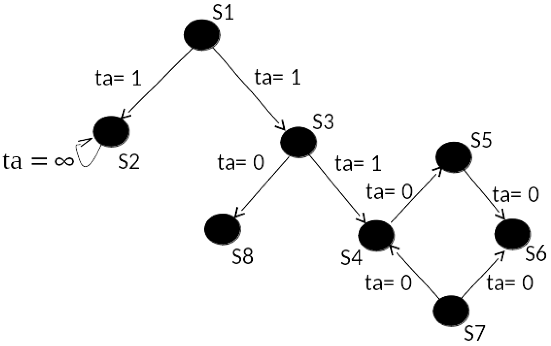
However, to address more fundamental issues, we need to start with a more primitive and perhaps more intuitive notion of a system. As in
Figure 2, consider a concept of system with states, transitions, and times associated with transitions. For example, there are transitions from state
S1 to state
S3 and from
S3 to
S4 which each takes 1 time unit and there is a cycle of transitions involving
each of which take zero time. There is a self-transition involving
S2 which consumes an infinite amount of time (signifying that it is passive, remaining in that state forever.) This is distinguished from the absence of any transitions out of
S8. A state trajectory is a sequence of states following along existing transitions, e.g.,
S1,
S3,
S4 is such a trajectory.
This example gives us a quick understanding of the conditions for system existence at the fundamental level.
We say that the system is:
not defined at S8 because there is no trajectory emerging from it;
non-deterministic at S1 because there are two distinct outbound transitions defined for it; and
deterministic at S2 and S4 because there is only one outbound transition for each.
We say that the system is
well-defined if it is defined at all its states. These conditions are relative to static properties, i.e., they relate to states not how the states follow one another over time. In contrast, state trajectories relate to dynamic and temporal properties. When moving along a trajectory, we keep adding the time advances to get the total traversal time, e.g., the time taken to go from
S2 to
S4 is 2. Here, a trajectory is said to be
progressive in time if time always advances as we extend the trajectory. For example, the cycle of states
is not progressive because as we keep adding the time advances the sum never increases. Conceptually, let us start a clock at 0 and, starting from a given state, we let the system evolve following existing transitions and advancing the clock according to the time advances on the transitions. If we then ask what the state of the system will be at some time later, we will always be able to answer if the system is well-defined and progressive. A well-defined system that is not progressive signifies that the system gets stuck in time and after some time, it becomes impossible to ask what the state of the system is in after that time. Zeno’s paradox offers a well-known metaphor where the time advances diminish so that time accumulates to a point rather than continue to progress and offers an example showing that the pathology does not necessarily involve a finite cycle. Our concept of progressiveness generalizes the concept of legitimacy for DEVS [
10] and deals with the “zenoness” property which has been much studied in the literature [
11]. We return to it in more detail later.
Thus, we have laid the conceptual groundwork in which a system has to be well-defined (static condition) and progressive (temporal dynamic condition) if it is to have achieved independent existence when emerging from a composition of components.
3. Iterative System Specifications
We briefly review an approach to Iterative Specification of Systems that was introduced in [
12] and provide more detail in
Appendix B. I/O systems describe system behavior with a global transition function that determines the final state given the initial state and the applied input segment. Since input segments are left segmentable and closed under composition, we are able to generate the state and output values along the entire input interval. However, such an approach is not very practical. What we need is a way to generate state and output trajectories in an iterative way going from one state along the trajectory to the next.
Iterative specification of systems is a general scheme for defining systems by iterative applications of generator segments. These are elementary segments from which all input segments of a system can be generated. Having such a concept we define a generator state transition function and iteratively apply generator segments to the generator state transition function. The results produced by the generator state transitions constitute the state trajectory for the input segment resulting from the composition of the generator segments. The general scheme of iterative specification forms a basis for more specialized types of specifications of systems. System specification formalisms are special forms of iterative specifications with their special type of generator segments and generator state transition functions.
Consider the set of all segments . Here, the notation, means that ω is a mapping from an interval of time base, T to a set of values Z. For a subset Γ of , the concatenation closure of Γ is denoted . Example generators are bounded continuous segments, and constant segments of variable length generating bounded piecewise continuous segments piecewise constant segments, respectively. Unfortunately, if Γ generates Ω, we cannot expect each to have a unique decomposition by Γ. A single representative, or canonical decomposition can be computed using a Maximal Length Segmentation (MLS). First we find , the longest generator in Γ that is also a left segment of ω. This process is repeated with what remains of ω after is removed, generating , and so on. If the process stops after n repetitions, then . We say that Γ is an admissible set of generators for Ω if Γ generates Ω and for each , a unique MLS decomposition of ω by Γ exists.
The following is the basis for further analysis in this paper:
Theorem 1. Sufficient Conditions for Admissibility. If Γ satisfies the following conditions, it admissibly generates : An
iterative specification of a system is a structure
where
T,
X,
Y, and
Q have the same interpretation as for I/O systems,
is an admissible set of input segment generators,
is the single segment state transition function, and
is the output function.
An iterative specification specifies a time invariant system, . The system is well-defined if , the extension of , has the composition property, i.e., , for all .
3.1. DEVS Simulation of Iterative Specification
As reviewed in
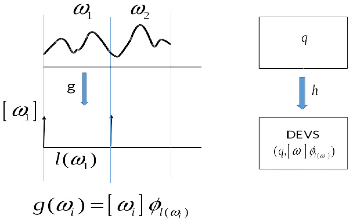
Appendix B, the notion of iterative specification was introduced to characterize diverse classes of systems such as differential equation systems and discrete time systems. With the motivation of including discrete event systems under the same umbrella as more familiar systems, DEVS was defined using iterative specification. Here we show that the converse is also true, namely, that DEVS can directly represent iterative specifications. Given an iterative specification
, we construct a DEVS model
that can simulate it in a step-by-step manner moving from one input segment to the next. The basic idea is that we build the construction around an encoding of the input segments of
G into the event segments of
M as illustrated in
Figure 3. This is based on the MLS which gives a unique decomposition of input segments to
G into generator subsegments. The encoding maps the generator subsegments.
ω in the order they occur into corresponding events which contain all the information of the segment itself. To do the simulation, the model
M stores the state of
G. It also uses its external transition function to store its version of
G’s input generator subsegment when it receives it.
M then simulates
G by using its internal transition function to apply its version of
G’s transition function to update its state maintaining correspondence with the state of
G.
Details of the construction are provided in
Appendix C. We note that the key to the proof is that iterative specifications can be expressed within the explicit event-like constraints of the DEVS formalism, itself defined through an iterative specification. Thus DEVS can be viewed as the computational basis for system classes that can be specified in iterative form satisfying all the requirements for admissibility.
3.2. Coupled Iterative Specification
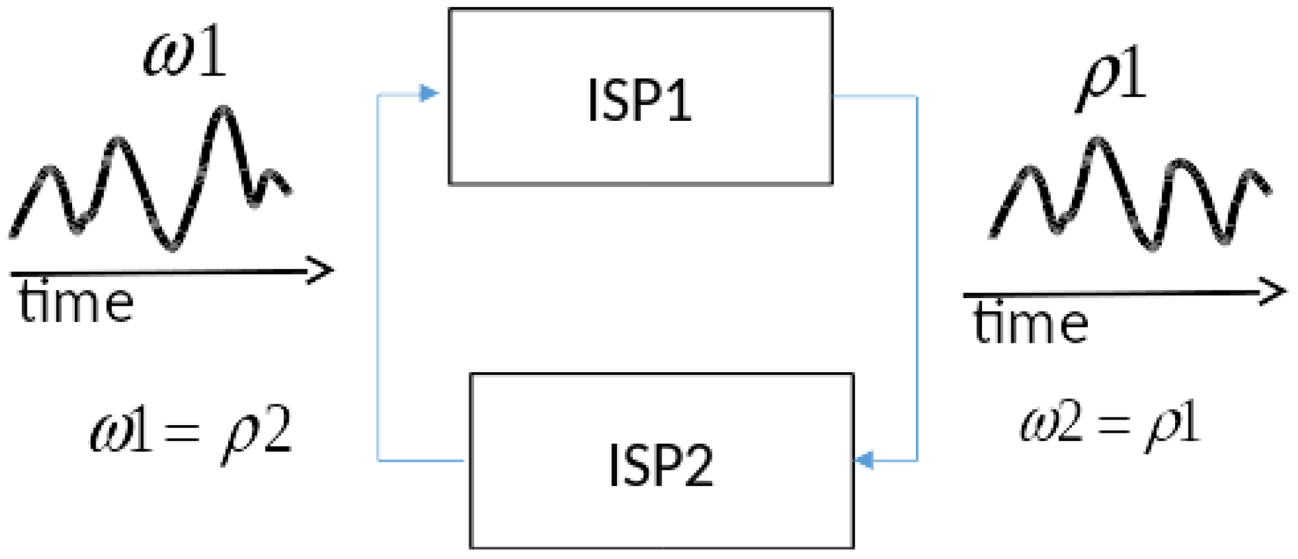
Although closure of coupling holds for DEVS, the generalization to iterative specification does not immediately follow. The problem is illustrated in
Figure 4 where two iterative system specifications, ISP1 and ISP2, are cross-coupled such as exemplified by the Turing machine example in
Figure 1. The cross-coupling introduces two constraints shown by the equalities in the figure, namely, the input of ISP2,
must equal the output of ISP1,
, and the input of ISP1,
must equal the output of ISP2,
. Here we are referring to input and output trajectories over time as suggested graphically in
Figure 4. Since each system imposes its own constraints on its input/output relation, the conjunction of the four constraints (two coupling-imposed, two system-imposed) may have zero, one, or multiple solutions.
Definition 1. A Coupled Iterative Specification is a network specification of components and coupling where the components are iterative specifications at the I/O System level.
As indicated, in the sequel, we deal with the simplified case of two coupled components. However, the results can be readily generalized with use of more complex notation. We begin with a definition of the relation of input and output segments that a system imposes on its interface. We need this definition to describe the interaction of systems brought on through the coupling of outputs to inputs.
Definition 2. The I/O Relation of an iterative specification is inherited from the I/O Relation of the system that it specifies. Likewise, the set of I/O Functions of an iterative specification is inherited from the system it specifies. Formally, let be the system specified by . Then the I/O Functions associated with G is where for , .
Let represent the I/O functions of the iterative specifications, ISP1 and ISP2, respectively. Applying the coupling constraints expressed in the equalities above, we make the definition:
Definition 3. A pair of output trajectories (ρ1,ρ2) is a consistent output trajectory for the state pair (q1,q2) if ρ1 = β1(q1,ρ2) and ρ2 = β2(q2,ρ1).
Definition 4. A Coupled Iterative Specification has unique solutions if there is a function, F:Q1 × Q2 → Ω; with F(q1,q2) = (ρ1,ρ2), where there is exactly one consistent pair (ρ1,ρ2) with infinite domain for every initial state (q1,q2). Infinite domain is needed for convenience in applying segmentation.
Definition 5. A Coupled Iterative Specification is admissible if it has unique solutions.
Theorem 2. An admissible Coupled Iterative Specification specifies a well-defined Iterative Specification at the I/O System level.
Theorem 3. The set of Iterative Specifications is closed under admissible coupling.
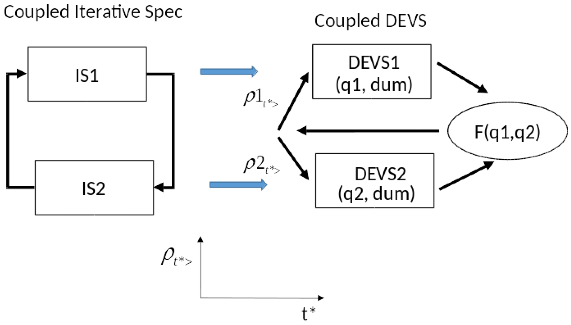
Theorem 4. DEVS coupled model can component-wise simulate a coupled Iterative Specification.
Proof. The coupled model has components, which are DEVS representations of the individual Iterative Specifications (according to Theorem D in
Appendix D) and also a coordinator as shown in
Figure 5.
The coordinator receives the current states of the components and applies the
F function to compute unique consistent output segments. After segmentation using the MLS as in the proof of Theorem D in
Appendix D, it packages each as a single event in a DEVS segment as shown. Each DEVS component computes the state of its Iterative Specification at the end of the segment as in Theorem D. Then it sends this state to the coordinator and the cycle repeats. This completes an informal version of the proof which would formally proceed by induction. □
The solution function
F represents an idealization of the fixed point solutions required for Differential Equation System Specification (DESS) and the local solution approaches of Discrete Time System Specification (DTSS) and Quantized DEVS [
12]. Generalized Discrete Event System Specification (GDEVS) [
13] polynomial representation of trajectories is the closest realization but the approach opens the door to realization by other trajectory prediction methods.
3.3. Special Case: Memoryless Systems
Consider the case where each component’s output does not depend on its state but only on its input.
Let
represent the ground state in which the device is always found (all states are represented by this state since output does not depend on state.) In the following
R1 and
R2 are the I/O relations of systems 1 and 2, respectively. In this case, they take special forms:
|
|
|
|
|
i.e.,
is consistent
Let
f and
g be defined in the following way:
|
|
So for any , and (considered as a relation).
Finally,
has:
no solutions if does not exist, yielding no resultant;
a unique solution for every input if exists, yielding a deterministic resultant; and
multiple solutions for a given segment is multivalued, yielding a non-deterministic resultant.
For examples, consider an
adder that always adds 1 to its input, i.e.,
|
|
Cross-coupling a pair of adders does not yield a well-defined resultant because . However, coupling an adder to a subtracter, its inverse, , yields a well-defined deterministic system.
For other examples, consider combinatorial elements whose output is a logic function of the input and consider a pair of gates of the same type connected in a feedback loop:
A NOT gate has an inverse , so the composition has two solutions one for each of two complementary assignments, i.e., yielding a non-deterministic system.
An AND gate with one of its input held to 0 always maps the other input into 0 so has a solution only for inputs of 0 to each component, i.e., , yielding a deterministic system.
An AND gate with a stuck-at input of 1 is the identity mapping and has multiple solutions i.e., , yielding a non-deterministic system.
3.4. Active-Passive Systems
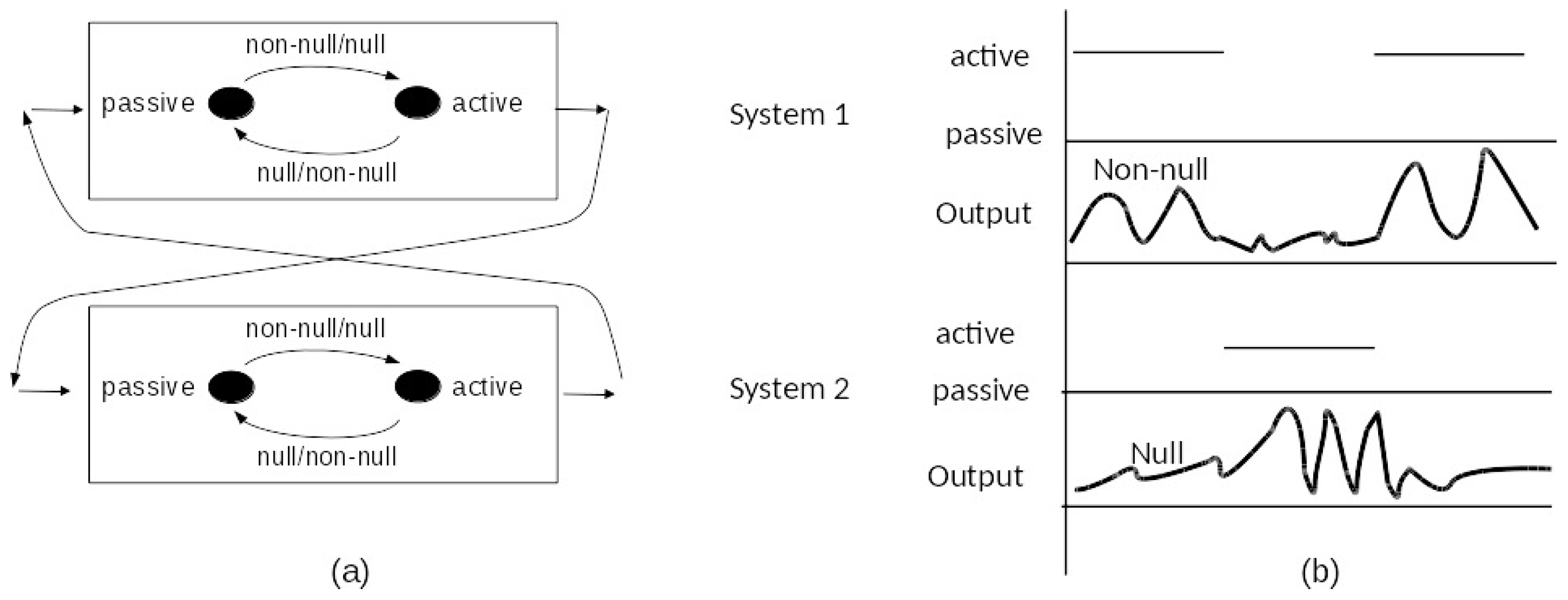
We now show that active–passive systems as described earlier offer a class of systems for which the iterative specifications of components satisfy the admissibility conditions specified in Theorem 4. As in
Figure 6a, consider a pair of cross-coupled systems each having input generators that represent null and non-null segments.
A null generator represents the output of a passive system whereas a non-null generator represents the output of an active system. For example in the TM case, a non-null generator is a segment that represents transmission of a symbol by the tape unit and of a symbol, move pair for the TM control. As in
Figure 6b let
S1 and
S2 start as active and passive, respectively. Then, they output non-null and null generators, respectively. Since the null generator has infinite extent, the end-time of the non-null generator determines the time of next event,
t* (as defined earlier) and we apply the transition functions in
Figure 6a to find that at
t* the systems have reversed phases with
S1 in passive and
S2 in active.
Definition 6. Define a triple by with with = endtime of the non-null generator segment
Let the non-null and null generators stand for sets of concrete segments that are equivalent with respect to state transitions and outputs. Then, such a scheme can define a deterministic or non-deterministic resultant depending on the number of consistent pairs of (non-null, null) generator segments are possible from the (active, passive) state. Furthermore, mutatis-mutandis for the state (passive, active).
4. Temporal Progress: Legitimacy, Zenoness
Although we have shown how a DEVS coupled model can simulate a coupling of iterative specifications, it does not guarantee that such a model is legitimate [
12]. Indeed, backing up, legitimacy of the simulating DEVS is reflective of the temporal progress character of the original coupling of specifications. We see that the time advance has a value provided that the function
F is defined for current state. However, as in the case of zenoness, a sequence of such values may accumulate at a finite point thus not allowing the system to progress beyond this point. Consequently, we need to extend the requirements for coupled iterative specifications to include temporal progress in order to fully characterize the resultant composition of systems. Thus, we can extend the definitions:
Definition 7. An Iterative Specification is progressive if every sequence of time advances diverges in sum.
Definition 8. A Coupled Iterative Specification is progressively admissible if its components are each progressive and the resultant Iterative Specification at the I/O System level is progressive.
Definition 9. A progressive Iterative Specification can be simulated by a legitimate DEVS.
Definition 10. A progressively admissible Coupled Iterative Specification can be component-wise simulated by a legitimate DEVS.
Zeigler et al. [
12] showed that the question of whether a DEVS is legitimate is undecidable. The approach was to express a Turing Machine as a DEVS and showing that solving the halting problem is equivalent to establishing legitimacy for this DEVS. We can transfer this approach to the formulation of the TM in
Figure 1 by setting the time advances of both components to zero except for a halt state which is a passive state (and has an infinite time advance). Then a TM DEVS is legitimate just in case the TM it implements ever halts. Since there is no algorithm to decide whether an arbitrary TM will halt or not the same is true for legitimacy. Since DEVS is an iterative specification, the problem of determining whether an Iterative Specification is progressive is also undecidable. Likewise, the question of whether a coupled iterative specification is progressive is undecidable.
Fundamental Systems Existence: Probabilistic Characterization of Halting
The existence of an iteratively specified system requires temporal progress and there is no algorithm to guarantee in a finite time that such progress is true. The underlying point is that, given an arbitrary TM, we have to simulate it step-by-step to determine if it will halt. Importantly, if a TM has not halted after some time, however long, this gives us no further information on its potential halting in the future. However, while this is true for individual TMs, the situation may be different for the statistics of subclasses of TMs. In other words, for a given class of TMs, the probability of an instance halting may be found to increase or decrease for the future given that it has not yet halted.
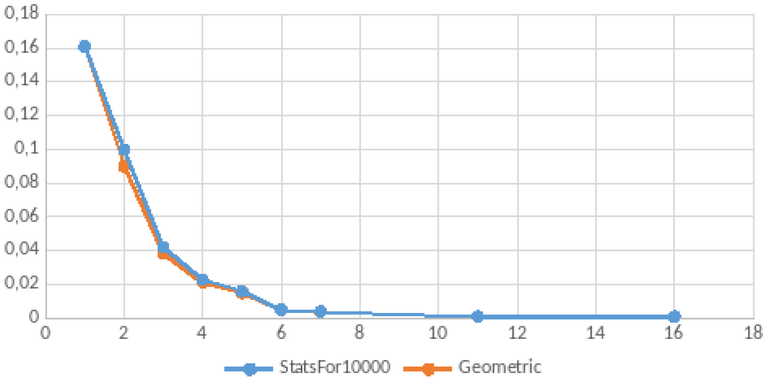
We performed an empirical study of randomly generated TMs described in
Appendix E. The results seem to show that TMs break into two classes—those that halt within a small number of steps (e.g., 16) and those that do not halt. Indeed, the data suggest that approximately one-third of the sampled TMs halt, while two-thirds do not. For those that halt, the probability of halting at the first step is greatest and then decreases exponentially and so is well-described by a geometric distribution with probability of success approximately
. In other words the probability of halting is
at each step given the TM has not halted earlier for the set that will eventually halt.
Summarizing, the existence of an iteratively specified system is not algorithmically decidable but there may be useful probabilistic formulations that can be applied to sub-classes of such specifications. For example, it seems to be that with high probability the halting of a two-symbol, three-state TM can be decided within 16 simulation steps. Therefore, it might be tractable for an assemblage of components to find a way to solve its composition problems in a finite time for certain classes of components couplings.
5. Discussion: Future Research
The discussion presented here was limited to compositions having two components with cross-coupled connections. However, this scope was sufficient to expose the essential effect of feedback in creating the need for consistent assignments of input/output pairs and the additional—distinct—requirement for time progression. Further development can extend the scope to arbitrary compositions generalizing the statement of consistent assignments to finite and perhaps, infinite sets of components.
Further, when extending to arbitrary composition sizes, the analysis revealing fundamental conditions for the emergent existence of systems from component systems suggests new classes of systems that can be defined using iterative specifications. For example, we might consider the active–passive systems in a more general setting. First allowing any finite number of them in a coupling can satisfy the requirement for at most one active component at any time by restricting the coupling to a single influencer for each component. In fixed coupling exhibiting feedback, this amounts to a cyclic formation in which activity will travel around the cycle from one component to the next. Another common pattern is a single component (root) influencing a set of components (branches) each of which influences only the root. Several possibilities for interaction of the root with the branches can result in admissible compositions. For example, the root might select a single branch to activate to satisfy the single active component requirements. Alternatively, it might activate all branches and count the number of branches as they successively go passive, becoming active when all the branches have become passive. These alternative configuration require knowledge of the protocol underlying the interaction but this only means that proofs of emergent well-defined resultants will be conditioned to narrower sub-classes of systems rather than to broad classes such as all differential equation systems.
After much progress in understanding how dynamic structure can be managed in DEVS-based simulations [
14,
15,
16], a framework that incorporates several insights has recently been developed [
17]. This framework, formulated in the DEVS formalism, can be extended to iterative specifications and investigated for conditions of existence as done here. The extension will probably increase the complexity required to state and establish the conditions but would, if successful, bring us closer to understanding the emergence of systems from assemblages of components in the real world.


