Sustainability Assessment of Asset Management Decisions for Wastewater Infrastructure Systems—Development of a System Dynamic Model

Abstract
:1. Introduction
2. Review of SD Models of Water Infrastructure System
3. Ganjidoost SD Model Advancement
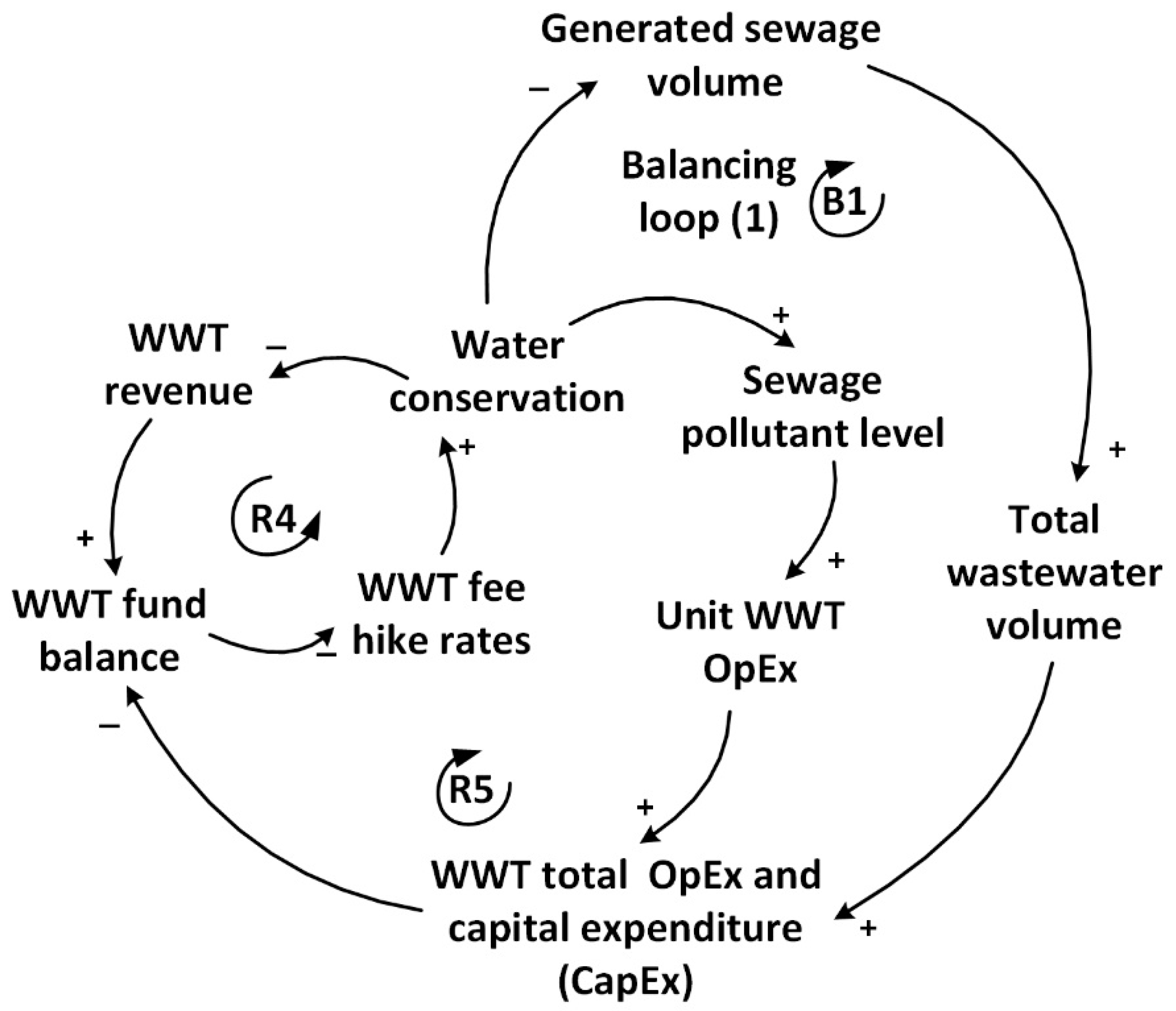
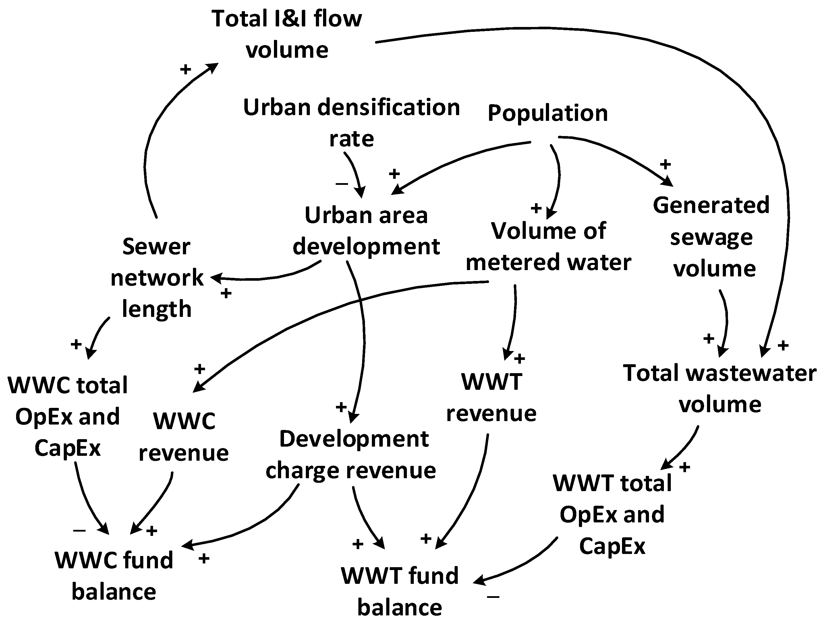
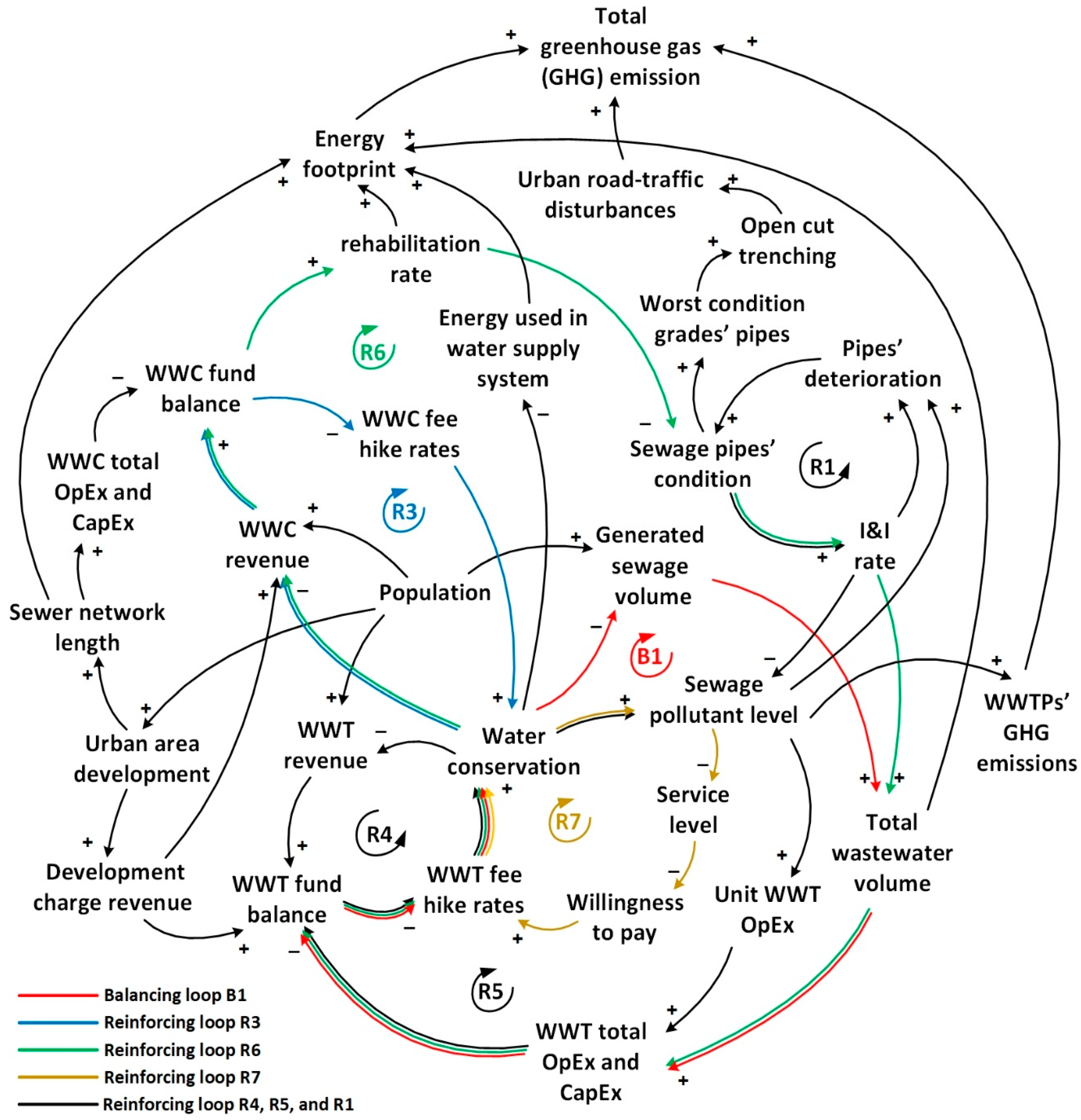
3.1. CLD Development
3.2. SD Model Parameterization
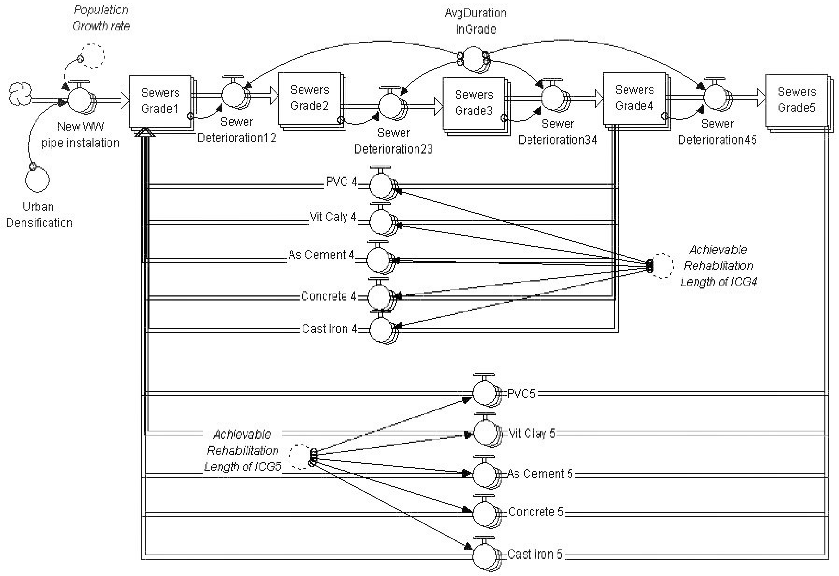
3.2.1. Physical Infrastructure Sector
WWC Physical Model
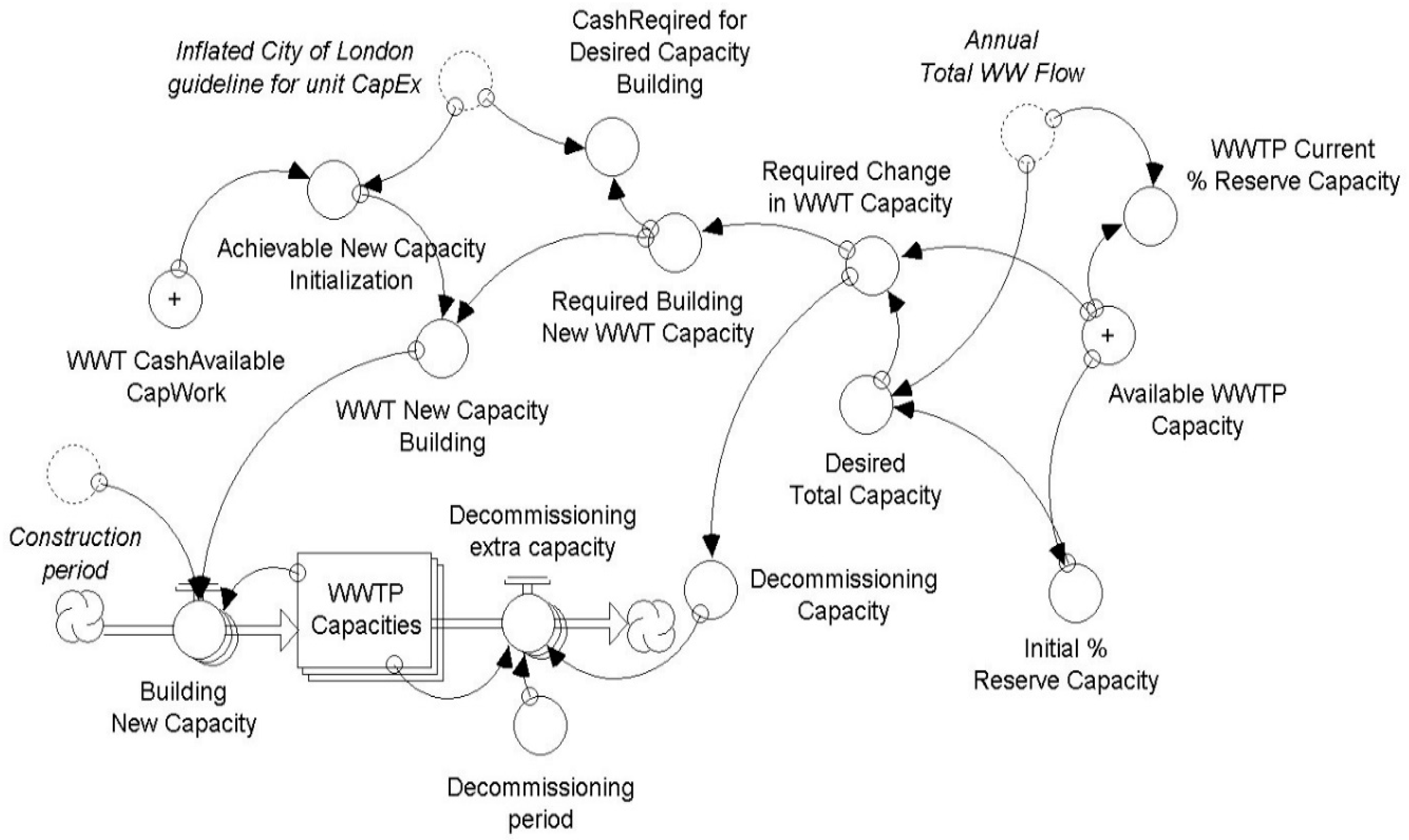
WWTP Physical Model
Wastewater Composition Model
- t [year] is the current time;
- SS (t) [g/l] is the concentration of suspended solid in wastewater inflow at WWTP in year t;
- SS0 [kg/capita/year] is the initial mass of suspended solid generation per capita;
- 365/1000 [(day/year)/(m3/liter)] is the conversion factor to convert days to year and liter to cubic meter;
- WD (t) [liter/capita/day] is the average daily water demand of a residential user in year t;
- CUF [%] is the percentage of water received by customers that is not returned as sewage to the WWC pipe network;
- I&I [m3/year] is the annual inflow and infiltration volume to the WWC pipe network;
- Population (t) is the population number in year t.
- t [year] is the current time;
- BOD [kg/capita/year] is the mass of dissolved oxygen needed by aerobic biological organisms to break down organic material presented in wastewater sample in year t;
- BOD0 [kg/capita/year] is the initial BOD;
- 365/1000 [(day/year)/(m3/liter)] is the conversion factor to convert days to year and liter to cubic meter;
- WD (t) [liter/capita/day] is the average daily water demand of a residential user in year t;
- CUF [%] is the percentage of water received by customers that is not returned as sewage to the WWC pipe network;
- I&I [m3/year] is the annual inflow and infiltration volume to the WWC pipe network;
- Population (t) is the population number in year t.
3.2.2. Consumer Sector
3.2.3. Finance Sector
WWC Finance Model
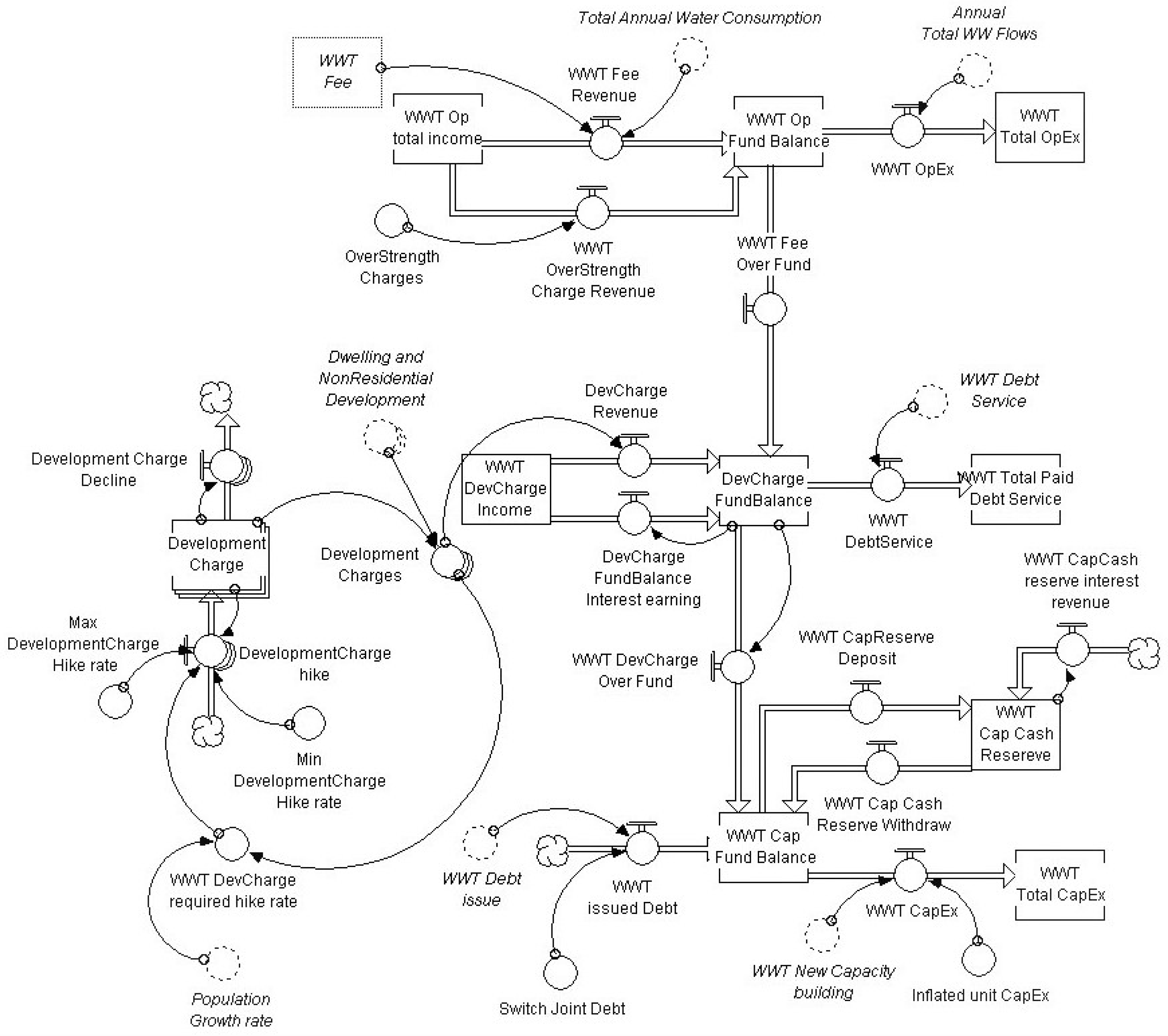
WWTP Finance Model
- t [year] is the current time;
- DCresidential (t) [$/year] represents the revenue of issuing permits for residential building constructions in year t;
- Nresidential [household/year] is the number of households added to the current population in year t;
- UDI [%] represents the urban densification index;
- S(t) [$] is the development-charge for single and attached houses in year t;
- A(t) [$] is the development-charge for apartments and lodging units in year t.
- t [year] is the current time;
- DCnon-residential (t) [$/year] represents the revenue of issuing permits for construction of non-residential buildings in year t;
- ADnon-residential [m2/year] is the new area permitted for building commercial, institutional or industrial buildings in year t;
- UDI [%] represents the urban densification index;
- NR (t) [$/m2] is the development-charge for non-residential area development in year t.
3.2.4. Environment Sector
GHG Calculation Model
- ○
- Annual GHG emission from WWT processes;
- ○
- Annual GHG emission from electric energy-use;
- ○
- Annual GHG emission from ICG5 pipes’ replacement, new pipes’ installations, and ICG4 pipes’ rehabilitation.
GHG Emission from WWT Processes:
- t [year] is the current time;
- CH4 (t) [kg/year] represents the mass of methane gas emissions in year t;
- Ui [%] represent the fraction of population in income group i as rural, urban high income, and urban low income;
- Tij [%] indicates the treatment pathway j as centralized well managed aerobic treatment, overloaded aerobic treatment, anaerobic digester, etc., served for each group of people in different income groups or (i);
- EFj [kg/year] is the emission factor in each treatment pathway;
- IBOD(t) [mg/l] is the BOD concentration of wastewater inflow at WWTP in year t;
- SBOD(t) [mg/l] is the BOD in removed sludge from WWTP in year t;
- R [kg CH4 /year] represents the recovered methane gas from WWTP in each studied year.
- t [year] is the current time;
- N2O (t) [kg/year] represents the mass of nitrous oxide emissions in year t;
- P (t) [capita] is the population in year t;
- 0.004 [kg/capita/year] is the mass of nitrous oxide emission per person per year (industrial and commercial discharges are also attributed to the residential users).
- t [year] is the current time;
- GHG (t) [kg/year] represents the equivalent mass of CO2 gas emitted from WWT processes in year t;
- 23 [kg CO2/kg CH4] represents the relative global warming potential of CH4 gas compared to an equivalent mass of CO2 gas;
- CH4 (t) [kg/year] is the annual CH4 emission calculated in Equation (5);
- 296 [kg CO2/kg N2O] represents the relative global warming potential of N2O gas compared to an equivalent mass of CO2 gas;
- N2O [kg/year] is the annual N2O emission calculated in Equation (6).
GHG Emission from Electric Energy Use:
- Annual_Energy_use_for_sewage_capital_works [gigajoule/year], which includes the energy used for new pipes installation and ICG4 pipes rehabilitation activities;
- Annual_Energy_used_for_sewage_collection [gigajoule/year];
- Annual_Energy_used_for_WWT [gigajoule/year];
- Annual_energy_used_for_WT [gigajoule/year];
- Annual_energy_used_for_water_distribution [gigajoule/year];
- Annual_Energy_use_for_sludge_transportaiton [gigajoule/year] to a central treatment facility such as incineration plant or landfill site;
- Sludge_treatment_Energy [gigajoule/year] produced or used in sludge treatment processes.
GHG Emissions from Pipes’ Installation, Replacement, and Rehabilitation:
- t [year] is the current time;
- GHG_raod_ststem (t) [kg/year] represents the equivalent mass of CO2 emitted from traffic disturbances in year t;
- 2 [kg CO2eq.)/m] represents the GHG emission factor for rehabilitation of ICG4 pipes in year t by using trenchless technologies;
- ICG4 (t) [m/year] is the length of ICG4 pipes rehabilitated in year t;
- 64 [kg CO2/m] represents the GHG emission factor for replacement of ICG5 or installation of new WWC pipes using open-cut technology in year t (daily traffic is assumed to be 3500 vehicles/day);
- ICG5 [m/year] is the length of ICG5 pipes being replaced in year t;
- NSP [m/year] is the length of new WWC pipes being installed in year t.
4. SD Model Interface
4.1. Initial Data Entries
4.2. Policy Levers
4.3. Advanced SD Model Outputs
5. Conclusions
- (1).
- (2).
- It advances the scope of the SD models presented in [20,22], to include the environmental consequences of strategic decisions related to asset management planning of wastewater infrastructure system. Additionally, new policy levers, such as population growth and urban densification in the social sector, and minimum fee-hike rates in the finance sector, are employed to enhance the representation of real-world conditions in the asset management planning process.
- (3).
- The newly developed CLDs will help decision makers to better understand the interrelated behavior of social, environmental, and economic systems, so they can see the whole picture and communicate the issues more effectively to other stakeholders.
- (4).
- The present SD model is developed as part of the asset management planning framework shown in Figure 1. Application of this model will allow the asset management planners to project the performance of WWC assets onto their future life-cycle, assess the sustainability of strategic asset management decisions, and find synergistic savings and opportunities when planning for the sustainability of these assets.
Author Contributions
Funding
Acknowledgments
Conflicts of Interest
References
- Government of Canada. Federal Sustainable Development Act; Government of Canada: Ottawa, ON, Canada, 2008.
- Government of Canada. Federal Sustainable Development Strategy. Available online: http://fsds-sfdd.ca/index.html#/en/goals/ (accessed on 7 May 2018).
- (CSCE) CSCE’s Vision 2020. Available online: https://csce.ca/wp-content/uploads/2018/08/Vision-2020-member-information-August-10-12-jak2.pdf (accessed on 10 May 2019).
- Federation of Canadian Municipalities. How to Develop an Asset Management Policy, Strategy and Governance Framework: Set Up A Consistent Approach to Asset Management in Your Municipality; Federation of Canadian Municipalities: Ottawa, ON, Canada, 2018. [Google Scholar]
- Federation of Canadian Municipalities. Leadership in Asset Management Program. Available online: https://fcm.ca/home/programs/green-municipal-fund/resources-and-programs/leadership-in-asset-management-program.htm (accessed on 7 May 2018).
- FCM. Municipalities for Climate Innovation Program (MCIP). Available online: https://fcm.ca/home/programs/municipalities-for-climate-innovation-program/municipalities-for-climate-innovation-program.htm (accessed on 25 May 2018).
- Felio, G.; Lounis, Z. Model Framework for Assessment of State, Performance, and Management of Canada’s Core Public Infrastructure; NRC: Washington, DC, USA, 2009. [Google Scholar]
- ISO 55000. Assessments and Road mapping Services. Available online: https://www.assetmanagementstandards.com/assessments-roadmapping/ (accessed on 23 February 2018).
- Halfawy, M.M.R.; Newton, L.A.; Vanier, D.J. Review of Commercial Municipal Infrastructure Asset Management Systems. Electron. J. Inf. Technol. Constr. 2006, 11, 211–224. [Google Scholar]
- Sala, S.; Ciuffo, B.; Nijkamp, P. A Meta-Framework for Sustainability Assessment Research Memorandum; VU University: Amsterdam, The Netherlands, 2013. [Google Scholar]
- Upadhyaya, J.K. A Sustainability Assessment Framework for Infrastructure: Application in Stormwater Systems. Ph.D. Thesis, University of Windsor, Windsor, ON, Canada, 2013. [Google Scholar]
- Mohammadifardi, H.; Knight, M.A.; Unger, A.J.A. Development of an asset management planning tool for integrated wastewater collection and treatment systems. In Proceedings of the 36th International Conference of the System Dynamics Society, Reykjavík, Iceland, 7–9 August 2018; pp. 2150–2178. [Google Scholar]
- Mirchi, A.; Madani, K.; Watkins, D.; Ahmad, S. Synthesis of System Dynamics Tools for Holistic Conceptualization of Water Resources Problems. Water Resour. Manag. 2012, 26, 2421–2442. [Google Scholar] [CrossRef]
- Chung, G.; Lansey, K.; Blowers, P.; Brooks, P.; Ela, W.; Stewart, S.; Wilson, P. A general water supply planning model: Evaluation of decentralized treatment. Environ. Model. Softw. 2008, 23, 893–905. [Google Scholar] [CrossRef]
- Biachia, C.; Montemaggiore, G.B. A system dynamics-based simulation experiment for testing mental model and performance effects of using the balanced scorecard. Syst. Dyn. Rev. 2008, 24, 175–213. [Google Scholar]
- Das, B.K.; Bandyopadhyay, M.; Mohapatra, P.K.J. System Dynamics Modeling of Biological Reactors for Waste Water Treatment. J. Environ. Syst. 1996, 25, 213–240. [Google Scholar] [CrossRef]
- Gillot, S.; De Clercq, B.; Defour, F.; Gernaey, K.; Vanrolleghem, P.; Jeppsonn, U.; Carstensen, J.; Carlsson, B.; Olsson, G. Optimization of Wastewater Treatment Plant Design and Operation Using Simulation and Cost Analysis. In Proceedings of the WEF Conference and Exposition, New Orleans, LA, USA, 9–13 October 1999; pp. 9–13. [Google Scholar]
- Parkinson, J.; Schütze, M.; Butler, D. Modelling the Impacts of Domestic Water Conservation on the Sustain Ability of the Urban Sewerage System. Water Environment J. 2005, 19, 49–56. [Google Scholar] [CrossRef]
- Rehan, R. Sustainable Municipal Water and Wastewater Management Using System Dynamics. Ph.D. Thesis, University of Waterloo, Waterloo, ON, Canada, 2011. [Google Scholar]
- Rehan, R.; Knight, M.A.; Haas, C.T.; Unger, A.J.A. Application of system dynamics for developing financially self-sustaining management policies for water and wastewater systems. Water Res. 2011, 45, 4737–4750. [Google Scholar] [CrossRef] [PubMed]
- Rehan, R.; Knight, M.A.; Unger, A.J.A.; Haas, C.T. Development of a system dynamics model for financially sustainable management of municipal watermain networks. Water Res. 2013, 47, 7184–7205. [Google Scholar] [CrossRef] [PubMed]
- Ganjidoost, A. Performance Modeling and Simulation for Water Distribution and Wastewater Collection Networks; University of Waterloo: Waterloo, ON, Canada, 2016. [Google Scholar]
- Ganjidoost, A.; Knight, M.A.; Unger, A.J.A.; Haas, C.T. Benchmark performance indicators for utility water and wastewater pipelines infrastructure. J. Water Resour. Plan. Manag. 2018, 144. [Google Scholar] [CrossRef]
- Rehan, R.; Unger, A.J.A.; Knight, M.A.; Haas, C.T. Strategic Water Utility Management and Financial Planning Using a New System Dynamics Tool. J. Am. Water Works Assoc. 2015, 107, 22–36. [Google Scholar] [CrossRef]
- Ganjidoost, A.; Haas, C.; Knight, M.; Unger, A. A System Dynamics Model for Integrated Water Infrastructure Asset Management. In Proceedings of the 33rd International Conference of the System Dynamics Society, Cambridge, MA, USA, 19–23 July 2015; pp. 1–16. [Google Scholar]
- Rehan, R.; Knight, M.A.; Unger, A.J.A.; Haas, C.T. Financially sustainable management strategies for urban wastewater collection infrastructure—Development of a system dynamics model. Tunn. Undergr. Space Technol. 2014, 39, 116–129. [Google Scholar] [CrossRef]
- Min, K.; Yeats, S.A. Water Conservation Efforts Changing Future Wastewater Treatment Facility Needs. Flourida Water Resour. J. 2011, 39–41. Available online: https://fwrj.com/techarticles/0811%20tech2.pdf (accessed on 10 May 2019).
- DeZellar, J.T.; Walter, J.M. Effects of Water Conservation on Sanitary Sewers and Wastewater Treatment Plants. Water Pollut. Control Fed. 1980, 52, 76–88. [Google Scholar]
- Marleni, N.; Gray, S.; Sharma, A.; Burn, S.; Muttil, N. Impact of water management practice scenarios on wastewater flow and contaminant concentration. J. Environ. Manag. 2015, 151, 461–471. [Google Scholar] [CrossRef] [PubMed]
- Rehan, R.; Knight, M.A. Do Trenchless Pipeline Construction Methods Reduce Greenhouse Gas Emissions; Centre for the Advancement of Trenchless Technologies (CATT) Department of Civil and Environmental Engineering, University of Waterloo: Waterloo, ON, Canada, 2007; p. 19. [Google Scholar]
- Richmond, B. An Introduction to Systems Thinking; Isee Systems, Inc.: Lebanon, NH, USA, 1997; ISBN 0970492111. [Google Scholar]
- WRc Sewerage Rehabilitation Manual; Water Research Centre: Swindon, UK, 2011.
- Recommended Standards for Wastewater Facilities; Health Research, Inc., Health Education Services Division: Albany, NY, USA, 2014.
- Statistics Canada Non-residential Building Construction Price Index, Fourth Quarter 2016. Available online: https://www150.statcan.gc.ca/n1/daily-quotidien/170214/dq170214a-eng.htm (accessed on 31 October 2018).
- Development Charges Act. Available online: https://www.ontario.ca/laws/statute/97d27 (accessed on 10 May 2019).
- Doorn, M.R.J.; Towprayoon, S.; Manso Vieira, S.M.; Irving, W.; Palmer, C.; Pipatti, R.; Wang, C. Chapter 6 Wastewater Treatment and Discharge. In Intergovernmental Panel on Climate Change (IPCC) Guidelines for National Greenhouse Gas Inventories; Institute for Global Environmental Strategies (IGES): Hayama, Japan, 2006; Volume 5. [Google Scholar]
- Environment Canada. 2011 Municipal Water Use Report; Environment Canada: Gatineau, QC, Canada, 2011. Available online: https://www.ec.gc.ca/doc/publications/eau-water/COM1454/survey8-eng.htm (accessed on 10 May 2019).
- Cashman, S.; Gaglione, A.; Mosley, J.; Weiss, L.; Hawkins, T.R.; Ashbolt, N.J.; Cashdollar, J.; Xue, X.; Ma, C.; Arden, S. Environmental and Cost Life Cycle Assessment of Disinfection Options for Municipal Wastewater Treatment; National Homeland Security Research Center: Cincinnati, OH, USA, 2014; ISBN 9781583219003.
- Sahely, H.R.; MacLean, H.L.; Monteith, H.D.; Bagley, D.M. Comparison of on-site and upstream greenhouse gas emissions from Canadian municipal wastewater treatment facilities. J. Environ. Eng. Sci. 2006, 5, 405–415. [Google Scholar] [CrossRef]
- Balkema, A.J.; Preisig, H.A.; Otterpohl, R.; Lambert, F.J.D. Indicators for the sustainability assessment of wastewater treatment systems. Urban Water 2002, 4, 153–161. [Google Scholar] [CrossRef]
- Sahely, H.R.; Kennedy, C.A.; Adams, B.J. Developing sustainability criteria for urban infrastructure systems. Can. J. Civ. Eng. 2005, 32, 72–85. [Google Scholar] [CrossRef]


| Data Entry | Unit | Practical Range |
|---|---|---|
| Life-cycle energy used for pipes manufacturing | MJ/kg | 50–100 |
| Life-cycle energy used for new pipe installation | MJ/m | 1000–2000 |
| Life-cycle energy use for drinking water treatment | MJ/m3 | 0–3 |
| Energy use for water distribution (WD) | MJ/m3 | 0–3 |
| Energy use for wastewater collection (WWC) | MJ/m3 | 0–1 |
| Life-cycle energy used for wastewater treatment | MJ/m3 | 0–3 |
| Life-cycle energy used for treatment plant construction | MJ/m3 | 0–1 |
| Life-cycle energy used for pipes manufacturing | MJ/kg | 50–100 |
| Data Entry | Unit | Practical Range |
|---|---|---|
| Initial length of pipes based on material and internal condition grade | Km | 0–103 |
| Initial number of water meters based on pipe diameter | - | 0–105 |
| Initial capacity of wastewater treatment plants (WWTPs) | m3/day | 0–1010 |
| Initial total infiltration and inflow | m3/year | 0–1010 |
| Initial equivalent suspended solid generation | kg/year/capita | 40–70 |
| Initial equivalent biological oxygen demand (BOD) generation | kg/year/capita | 50–70 |
| Data Entry | Unit | Practical Range |
|---|---|---|
| Initial population | capita | 0–5 × 10⁹ |
| Average household size | capita | 2–4 |
| Population growth rate | percent/year | 0–100 |
| Initial water demand for residential users | liter/day/capita | 150–300 |
| Minimum water demand for residential users | liter/day/capita | 100–150 |
| Initial water demand for non-residential users | liter/year | 0–5 × 10¹⁸ |
| Bill hardship threshold | % of household income | 0.1–100 |
| Initial number of residential apartment and lodging | - | 10–5 × 10⁵ |
| Initial number of houses and townhouses | - | 10–5 × 10⁵ |
| Initial non-residential area | m2 | 10–5 × 10⁷ |
| Initial WWC fee for residential user | $/m3 | 0.01–10 |
| Initial WWC fee for non-residential user | $/m3 | 0.01–10 |
| Initial WWT-free residential user | $/m3 | 0.01–10 |
| Initial WWT-free non-residential user | $/m3 | 0.01–10 |
| Data Entry | Unit | Practical Range |
|---|---|---|
| Price elasticity of water demand for residential users | - | 0–1 |
| Average household income | $/year | 50,000–90,000 |
| Initial WWC cost | $/m3 | 0.1–10 |
| Initial WWT cost | $/m3 | 0.1–10 |
| Initial debt/reserve of utility (for WWC model) | $ | 0–109 |
| Initial debt/reserve of region (for WWTP model) | $ | 0–109 |
| Annual revenues from industries for over strength wastewater discharge | $/year | 0–109 |
| Unit maintenance cost of WWC pipes in each ICG class | $/m/year | 2–10 |
| Unit development charge for apartments/lodges | $/unit | 1000–3000 |
| Unit development charge for houses/townhouses | $/unit | 2000–5 × 10⁴ |
| Unit development charges for non-residential areas | $/m2 | 0.1–10 |
| Initial service charges based on water meter sizes | $/m | 200–2000 |
| Unit cost of CIG4 pipes’ rehabilitation | $/m | 400–600 |
| Unit cost of ICG5 pipes replacement | $/m | 700–1000 |
| Inflation rate for electrical energy cost | - | 0–5 |
| Inflation rate for non-residential building construction cost | - | 0–7 |
| Fixed borrowing rate | - | 0–7 |
| Fixed saving rate | - | 0–5 |
| Price elasticity of water demand for residential users | - | 0–1 |
| Policy Lever | Unit | Range or Value |
|---|---|---|
| Physical sector | ||
| Preferred rehabilitation rate | % | 0–100 |
| Max acceptable ICG5 fraction | % | 0–100 |
| ICG5 elimination period | year | 0–100 |
| Rehab ICG4 switch | - | 0 or 1 |
| Finance sector | ||
| WWC allowable fee-hike rate | % | 0–100 |
| WWT max allowable fee-hike rate | % | 0–100 |
| WWT min allowable fee-hike rate | % | 0–(WWT max allowable fee hike rate) |
| Sewage treatment-fee decline switch | - | 0 or 1 |
| WWT max development-charge hike rate | % | 0–100 |
| WWT min development-charge hike rate | % | 0–(WWT max development-charge hike rate) |
| WWC desired capital-reserve fraction | % | 0–4 |
| WWT desired capital-reserve fraction | % | 0–100 |
| Consumer sector | ||
| Population growth rate | % | 0–100 |
| Urban densification rate | % | 0–100 |
| Variables | Unit | Description |
|---|---|---|
| Physical sector | ||
| Actual_Rehab_Rate (t) | % | Fraction of WWC pipe network that has been replaced or rehabilitated in year t |
| ICG5_Fraction (t) | % | Fraction of ICG5 pipes length that is in service within the WWC pipe network in year t |
| Avg_ICG_Network(t) | ICG | Average internal condition grade of the network in year t |
| Network_Expns(t) | m | Length of WWC pipe network expanded in year t |
| Generated_WW_Res (t) | m3/day | Sewage generated by residential users in year t |
| Generated_WW_Non-Res (t) | m3/day | Wastewater generated by non-residential users in year t |
| I&I(t) | m3/day | Inflow and infiltration volume in year t |
| Environment sector | ||
| Energy_Footprint | gigajoules | Total energy used in WWC and WWTP systems in year t |
| Total_GHG | tone CO2 | Total direct and indirect GHG emissions in year t |
| Finance sector | ||
| WWC_Fee (t) | $ | WWC fee hike rate for residential users in year t |
| WWT_Fee (t) | $ | WWT fee hike rate for residential users in year t |
| DevCharge_Res_Apt(t) | $ | Development charges for building new residential apartments in year t |
| DevCharge_Res_House(t) | $ | Development charges for building new residential houses in year t |
| DevCharge_NonRes(t) | $ | Development charges for development of non-residential areas in year t |
| WWC_Op_FB(t) | $ | Operational fund balance of WWC system in year t |
| WWC_Cap_FB(t) | $ | Capital fund balance of WWC system in year t |
| WWT_Op_FB(t) | $ | Operational fund balance of WWT system in year t |
| WWT_CevCharge_FB(t) | $ | Development charge fund balance of WWT system in year t |
| WWT_Cap_FB(t) | $ | Capital fund balance of WWT system in year t |
| WWC_Debt(t) | $ | Amount of issued debt for capital work expenses for WWC pipe network system in year t |
| WWT_Debt(t) | $ | Amount of issued debt for capital work expenses for WWTP capacity upgrading in year t |
| OpEx_WWC(t) | $ | Operational and maintenance expenses of WWC system in year t |
| CapEx_WWC(t) | $ | Capital expenses of WWC system in year t |
| OpEx_WWT(t) | $ | Operational and maintenance expenses of WWT system in year t |
| CapEx_WWT(t) | $ | Capital expenses of WWT system in year t |
| Reserve_WWT_Cap | % | Fraction of extra capacity in WWTP system in year t |
| Consumer sector | ||
| Water_demand_Res | l/c/d | Average daily water demand of residential users in year t |
| Bill_Burden | % | Fraction of an average household income which should be paid for WWC and WWT services |
© 2019 by the authors. Licensee MDPI, Basel, Switzerland. This article is an open access article distributed under the terms and conditions of the Creative Commons Attribution (CC BY) license (http://creativecommons.org/licenses/by/4.0/).
Share and Cite
Mohammadifardi, H.; Knight, M.A.; Unger, A.A.J. Sustainability Assessment of Asset Management Decisions for Wastewater Infrastructure Systems—Development of a System Dynamic Model. Systems 2019, 7, 26. https://doi.org/10.3390/systems7020026
Mohammadifardi H, Knight MA, Unger AAJ. Sustainability Assessment of Asset Management Decisions for Wastewater Infrastructure Systems—Development of a System Dynamic Model. Systems. 2019; 7(2):26. https://doi.org/10.3390/systems7020026
Chicago/Turabian StyleMohammadifardi, Hamed, Mark A. Knight, and Andre A.J. Unger. 2019. "Sustainability Assessment of Asset Management Decisions for Wastewater Infrastructure Systems—Development of a System Dynamic Model" Systems 7, no. 2: 26. https://doi.org/10.3390/systems7020026
APA StyleMohammadifardi, H., Knight, M. A., & Unger, A. A. J. (2019). Sustainability Assessment of Asset Management Decisions for Wastewater Infrastructure Systems—Development of a System Dynamic Model. Systems, 7(2), 26. https://doi.org/10.3390/systems7020026