The Contribution of Energy Taxes to Climate Change Policy in the European Union (EU)

Abstract

Energy taxes are one of the main market-based tools directed toward mitigating climate change in the European Union (EU). Therefore, the aim of this article was to analyze whether energy taxes really contribute to the reduction of greenhouse gas (GHG) emissions and the successful implementation of climate change policy. Applying the Granger causality test on time series and using panel data analysis, the direct and indirect (via the reduction of fossil energy consumption (FEC) and energy intensity (EI), as well as the increase of renewable energy consumption (REN)) impacts of energy taxes on GHG emissions in EU countries were analyzed in the present study. The results showed that energy taxes did not Granger-cause fossil energy consumption, energy intensity, renewable energy consumption, and GHG emissions in almost all EU countries. Regarding the panel data analysis, the results showed that energy taxes did not, directly and indirectly, influence GHG emissions. Therefore, this paper shows that generally, energy tax policy in EU countries is ineffective. Thus, tax policy should be reformed and matched with an emissions trading system in seeking climate change mitigation.

1. Introduction

In recent decades, climate change policy has attracted particular attention. Despite the increased number of studies on adaptation to climate change, the reduction of this problem remains the main task of environmental policy. The Intergovernmental Panel on Climate Change has stated that in order to not exceed global warming below 2 °C, greenhouse gas (GHG) emissions should be reduced between 80% and 95% by 2050 in developed countries, and meanwhile developing countries should stop the growth of GHG emissions. However, the main question is how to achieve these targets.

There are several policy tools for emissions control, many of which use economic mechanisms to influence environmental impacts. Environmental taxes are taxes imposed due to environmental reasons, and they provide an incentive to reduce certain environmental impacts. Environmental taxes affect resource consumption or emissions quantities by increasing the price of chargeable products [1,2,3] and are the tools most used in environmental policy. The main aim of these taxes is to change market prices to internalize environmental harms [4,5,6,7]. Increasing the prices of goods and services pushes consumers to change their purchasing behaviors, reducing demand for the products and services of polluters [8]. Furthermore, environmental taxes influence GHG emissions [3] by generating governmental income, which can be directed toward solving environmental issues and motivating taxpayers to improve production for social or economic purposes.

Energy taxes (defined as environmental taxes levied on energy products and on the production and consumption of energy) and carbon taxes (taxes levied on the burning of carbon-based fuels (coal, oil, gas)) are the market-based initiatives applied the most toward reducing the impact of climate change. The revenue of taxes ensures stable, long-term support for broad-based research focused on energy sources, energy use, and emissions reduction [9]. Therefore, these taxes are highly recommended by economists and international organizations as the most efficient market-based policy instruments [10]. Liang et al. [11] and Zhang and Li [12] have stated that these taxes could be an ideal economic tool in dealing with post-Kyoto pressure and are an effective measure in building a low-carbon economy. The EU has endorsed these measures in achieving the goals of environmental policy, as they are flexible and cost-effective [13,14]. Furthermore, the Paris Climate Agreement empowers nations to tax the carbon content of all goods without fear of retaliation [15].

Most studies have emphasized the impact of energy taxes on the emissions of GHGs, but the ambiguity of the results has provided a basis for deeper analysis of energy taxes. In this paper, we consider general energy taxes in order to reveal whether in separate EU countries and in all EU countries energy taxes contribute to climate change mitigation, which to the best of our knowledge has not been analyzed yet. Furthermore, in the literature, the direct and particularly indirect impacts of energy taxes on GHG emissions in the EU have been scarcely analyzed (see: [16,17,18]). Thus, the aim of this paper is to examine the impact of energy taxes on fossil energy consumption, energy intensity, renewable energy, and GHG emissions at the country level and the direct and indirect impacts of energy taxes on GHG emissions in all EU countries. This paper provides new insights into separate EU countries by revealing energy tax contributions to the implementation of climate policy.

The paper is organized as follows. Section 2 presents a literature review on the impact of energy taxes on the reduction of GHG emissions. Section 3 describes data and descriptive statistics about taxation in the EU. Section 4 explains the model and estimation strategy. Section 5 provides the estimation results. Section 5 presents discussion and policy implications. Section 6 concludes the paper.

2. Literature Review

Authors, while analyzing energy or carbon tax policy, usually examine the impact of taxes on the economy [7,12,19,20,21,22,23,24]. The majority of studies has emphasized the adverse effect of a high carbon tax rate on the economy [25]. Authors [11,26] have also indicated the negative effects of carbon and energy taxes on the international competitiveness of energy-intensive sectors and the occurrence of the leakage phenomenon [25]. Moreover, there have also been a number of studies analyzing the impacts of energy and carbon taxes on people’s welfare, employment [27,28,29,30], and inequality [20,31,32]. Oueslati et al. [30] have stated that energy taxes may lead to a loss of industry-specific human capital, thus increasing unemployment in the affected industries. Wesseh et al. [32] have shown that carbon taxes have a positive influence on a country’s welfare when the model reflects the benefits from environmental clean-up in all regions except for low-income countries. Therefore, it is very important to guarantee that taxes do not hinder economic growth and welfare [33,34]. However, when analyzing the taxes assigned to climate change mitigation, it is more important to evaluate the effectiveness of these taxes in reducing GHG emissions.

Considering climate change policy, carbon taxes are directly assigned to climate change mitigation [10,24,25,34,35,36] through taxes imposed on the carbon content in fossil fuels [37]. On the other hand, carbon taxes indirectly could affect changes in GHG emissions through carbon tax revenues subsidizing energy efficiency or renewable energy “green” spending [25,38]. A lot of authors have shown that carbon taxes reduce GHG emissions [7,10,15,22,23,24,25,30,35,36,39]. Meanwhile, Bruvoll and Larsen [36] have shown that GHG emissions decreased negligibly when Norway introduced a carbon tax, and the effects of a carbon tax in Denmark, Sweden, and the Netherlands were negative but not significant. However, carbon taxes with many exemptions have been introduced in EU countries, while energy taxes can be found in most EU countries.

Energy taxes do not directly focus on the reduction of GHG emissions and are only indirect GHG emissions taxes [38]. The taxation of energy is levied on many economic sectors, mainly energy and electricity production, transport, distribution, natural gas, and users ranging from large industrial users to households. Indirect GHG taxation is certainly a viable option in practice [40]. Fossil fuels (such as coal, oil, and natural gas) are the main target of energy taxes, as they are the main source of GHG emissions [40,41,42,43,44]. Thus, the most effective ways to control carbon emissions is to ensure energy saving and emissions reduction [19]. Carbon taxes are also included under energy taxes and are in many cases levied on the same tax bases as energy taxes and are substitutes for energy taxes. Moreover, Jeffrey and Perkins [43] have revealed that energy taxation has a larger positive impact on carbon emissions reduction than emissions trading systems (ETSes) or cap-and-trade systems do.

Energy taxes contribute to a decrease in GHG emissions in two ways, first by improving energy efficiency or using less fuel per unit of output (efficiency) [6,16,40,43,45,46,47]. Energy efficiency is one of the main determinants and is related to a reduction in GHG emissions [16,24]. Companies look for ways to reduce energy costs, implementing energy efficiency programs and facing additional costs [26]. However, the effectiveness of an energy tax policy depends on the price elasticity of energy demand [2]. Moreover, a tax has the advantage of generating revenue that could be used for promoting energy efficiency [37,41]. Thus, environmental taxes induce investment in abatement technologies and in increases in energy efficiency [32,48,49,50]. Technology is a crucial factor in assessing the long-run costs and benefits of environmental regulations [9,27]. On the other hand, a tax simulation of innovation-based businesses raises the demand for their products [51].

Second, energy taxes could contribute to a reduction in GHG emissions by increasing effectiveness if fuel with a lower carbon content is used [6,17,41,45]. Imposing a tax on fossil fuels increases the attractiveness of alternative fuels and creates an incentive for industrial users and households to choose more fuel-efficient products and processes [52]. The problem of implementing renewable energy (RE) investment is that most RE technologies are new and more costly, and therefore the rate of return on an RE project is lower on average when compared to fossil fuel [53]. The consumption of renewable energy is also a very important determinant in the reduction of GHG emissions. The increasing price of fuel caused by the energy tax leads to a decreased demand for polluted energy sources, caused by a substitution effect. A result of the implementation of this policy is the replacement of carbon-intensive fuels with “clean energy” (the process of optimization in an energy mix) [7]. Thus, energy taxes should promote a shift from carbon-intensive coal generation to carbon-free renewables, which leads to long-term increasing profitability of low-carbon renewable resources: Furthermore, this provides additional incentives in developing low-carbon resources such as renewables [6]. Moreover, energy tax revenues could subsidize environmental protection projects or technological developments in emissions reduction, supporting the development of renewable energy [10]. Resource consumption, which was developed by Tchorzewska-Cieslak et al. [54], was proven effective for pipelines as well as in achieving improved safety and reliability [55]), and emissions from fossil fuels related to supply chains decrease if, for example, a share of gasoline tax revenues is reinvested to subsidize biofuel production [52]. Thus, energy taxes create incentives for business investments to develop and use alternative low-carbon fuels and technologies [34]. In addition, when tax revenues are allocated to governmental investment funds, RE projects become more feasible and more interesting to investors, and hence the supply of investment money to these funds is increasing [53].

The direct impact of energy taxes on GHG emissions in the EU has been scarcely analyzed. Lapinskiene et al. [56] found that energy taxes in EU countries have a negative impact on pollution, which revealed that a higher value of energy taxes is associated with a lower level of GHGs. Jeffrey and Perkins [43] showed that as implicit tax rates on energy increased, the carbon intensity of emissions decreased in the EU. Sterner [52] also revealed that fuel taxes had a positive impact on carbon emissions reduction in Europe and Japan. In terms of indirect effects on GHG emissions, Jeffrey and Perkins [43] revealed that energy taxation does not directly affect the choice to use fuels with a lower carbon content. Meanwhile, energy taxes are associated with and lead to lower GHG emissions due to an increase in energy efficiency. Despite these findings, in climate change policy, a main question has been raised: Do energy taxes really contribute to the reduction of GHG emissions in general and in separate EU countries?

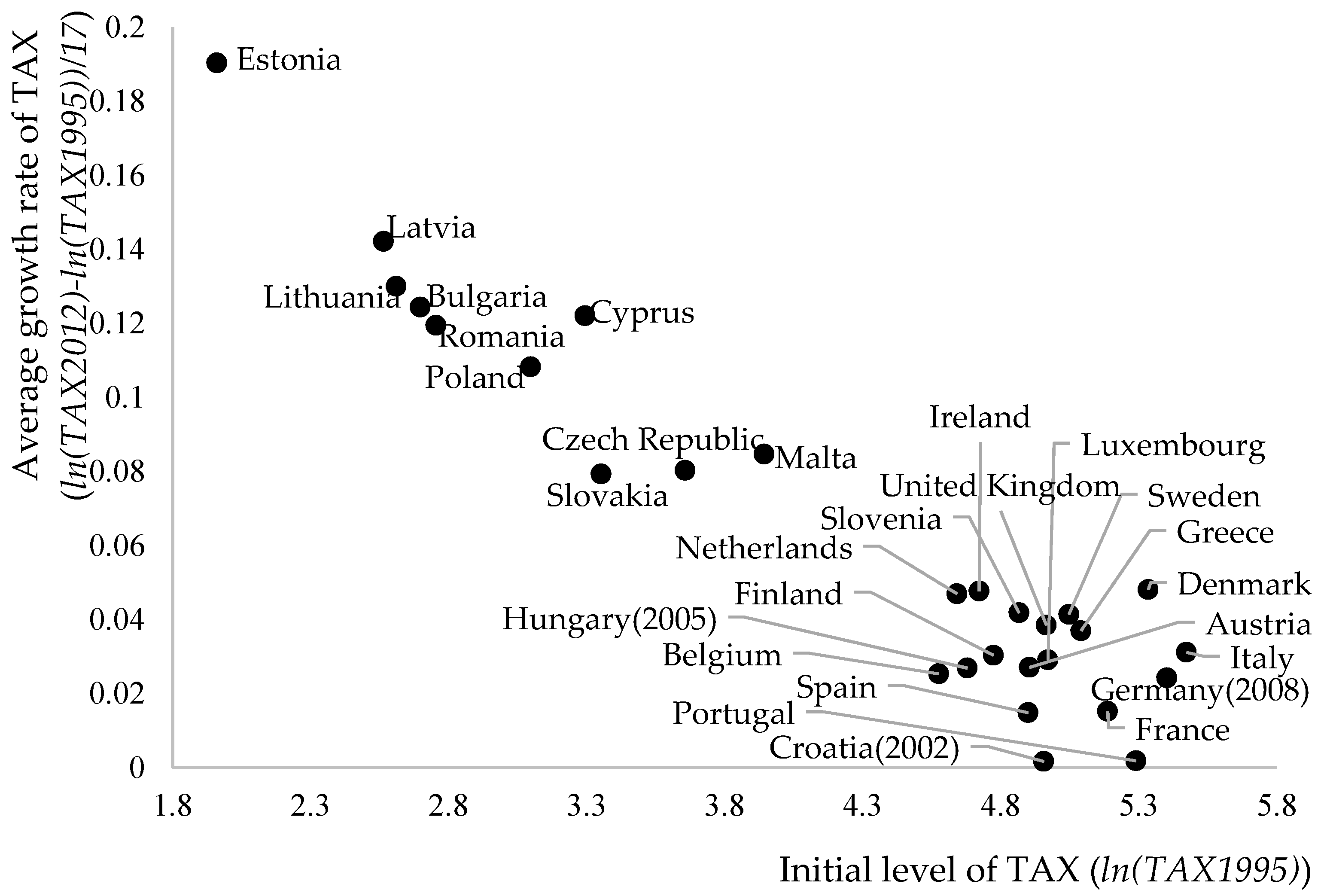
3. Data and Descriptive Statistics

For the analysis of the energy taxation impact on lowering energy intensity and fossil energy use, the promotion of renewable energy, and the final goal of reducing per capita GHG emissions, data were collected over the period 1995–2012 for 28 EU member states from the Eurostat and World Development Indicators (WDI) database to calculate the necessary variables (listed in

Table 1. Variables utilized in the analysis.

Variable Name	Short Variable Name	Explanation and Measurement Unit
Energy taxes	TAX	Euros per energy (except renewable and nuclear) ton of oil equivalent (TOE) consumed
Fossil energy consumption	FEC	Final energy (except renewable and nuclear) consumption per capita (tons of oil equivalent TOE)
Energy intensity	EI	Energy intensity of the economy (gross inland consumption of energy divided by gross domestic product (GDP) (kg of oil equivalent per 1000 EUR))
Renewable energy	REN	Share of renewable energy in gross inland consumption of energy (%)
Greenhouse gas emissions	GHG	Total greenhouse gas emissions per capita (tons of CO2 equivalent)

). The data for per capita GHG emissions were taken from the WDI database (http://data.worldbank.org). The data for all other variables were collected from the Eurostat database (https://ec.europa.eu/eurostat/data/database).

The descriptive analysis of these data is presented in

Table 2. Descriptive statistics.

Variable	Mean	Std. Dev.	Minimum	Maximum
TAX	162.7	83.0	6.6	502.9
FEC	7.1	25.1	0.9	163.2
EI	212.5	139.9	2.4	951.1
REN	8.49	6.5	0.1	27.2
GHG	11.03	4.2	4.9	28.9

. As can be seen, the mean of energy taxes in the EU was about 163 euro per energy ton, and the data were rather dispersive. During the analyzed period, one person in the EU on average consumed 7.1 tons of energy (TOE) and emitted 11 tons of GHGs. The average share of renewable energy in gross inland consumption of energy was 8.5%.

The changes in relative energy taxes in EU countries are presented in Figure 1. During the period 1995–2012, the relative taxation on energy grew in all EU member states. The most intensive growth was recorded in Estonia, where relative energy taxes increased even by 25 times. Meanwhile, the lowest growth of taxes was found in Croatia, Portugal, and Germany, where energy taxes increased only by 2%, 3%, and 10 %, respectively.

As we can see in Figure 2, the relationship between initial level of energy taxes and average growth rate over the analyzed period was negative, strong, and statistically significant (−0.948). This suggests that we observed a convergence of energy taxation levels between EU countries: i.e., the relative taxation on energy increased more in the countries where initially energy was not so heavily taxed.

4. Model and Estimation Method

Aiming to examine the impact that energy taxes (TAX) had on fossil energy consumption (FEC), energy intensity (EI) (that is reverse to energy efficiency), renewable energy (REN), and per capita greenhouse gas emissions (GHG) at a country level, we applied the Granger causality test to time series data. This test is a statistical hypothesis test for examining if one time series can be used to forecast another, and was proposed by Granger [57]. He argued that causality in economics could potentially be tested by assessing the capability to predict the future values of one time series by using the past values of another time series via ARDLM or ECM (ARDLM: Autoregressive distributed lag model; ECM: Error correction model; the selection of the model hinges on the presence of a cointegrated relationship). Energy taxes Granger-cause fossil energy consumption, energy intensity, renewable energy consumption, or GHG emissions if, through t-tests (in the cases where, besides a first-order lag model, a higher order lag of right-hand side variables is included, Granger causality is tested running an F-test on the joint insignificance of all estimated coefficients), once-lagged values of energy taxes give information about the future values of fossil energy consumption, energy intensity, renewable energy consumption, and GHG emissions that is statistically significant. This is quite intuitive if we take into account that for economic subjects, it takes time to adjust behavior to a new taxation policy (that could involve new tax rates or a broader tax base, as well as new tax rules), and this new policy could affect decisions with a time lag. Granger causality tests have been widely used to determine the direction of causal relationships between chosen variables. There have only been a few research works that have evaluated environmental tax impacts on reductions of greenhouse gas emissions at the EU level using the Granger causality method [58]. Previous research has usually analyzed the relationship between carbon emissions and economic growth ([59,60] among many others).

In the case of non-cointegrated time series for testing Granger causality, we applied ARDLM. We could detect that variables were cointegrated, also known as having a long-run stochastic trend, using a standard unit root test, e.g., an augmented (the level of augmentation is usually calculated as $\sqrt[3]{n}$) Dickey–Fuller (D-F) test following the Engel–Granger (E-G) four-step procedure (the unit–root hypothesis is not rejected for the individual time series, and the unit–root hypothesis is rejected for the residuals from the cointegrating regression). The general ARDLM takes the form of [61]

$$y_t=\gamma +\delta y_{t-1}+\phi x_{t-1}+{\epsilon }_t,$$

(1)

where y_t and x_t are stationary variables; γ, φ, and δ are parameters to be estimated; and ε_t is white noise. In cases where variables contain unit roots (but are not cointegrated), variables are used in first-differenced form to ensure stationarity. For capturing the possible nonlinear form of a relationship besides a level–level type of equation, we also estimated the equation in log–log form. Here, we were interested in φ, which, being statistically significant, would provide evidence that x Granger-causes y. Applying Equation (1) to our case, we have

$$FE{C}_t={\gamma }_1+{\delta }_{1}FE{C}_{t-1}+{\phi }_{1}TA{X}_{t-1}+{\epsilon }_t,$$

(2)

$$E{I}_t={\gamma }_2+{\delta }_{2}E{I}_{t-1}+{\phi }_{2}TA{X}_{t-1}+{\epsilon }_t,$$

(3)

$$RE{N}_t={\gamma }_3+{\delta }_{3}RE{N}_{t-1}+{\phi }_{3}TA{X}_{t-1}+{\epsilon }_t,$$

(4)

$$GH{G}_t={\gamma }_4+{\delta }_{4}GH{G}_{t-1}+{\phi }_{4}TA{X}_{t-1}+{\epsilon }_t,$$

(5)

$$TA{X}_t={\gamma }_5+{\delta }_{5}TA{X}_{t-1}+{\phi }_{5}FE{C}_{t-1}+{\epsilon }_t,$$

(6)

$$TA{X}_t={\gamma }_6+{\delta }_{6}TA{X}_{t-1}+{\phi }_{6}E{I}_{t-1}+{\epsilon }_t,$$

(7)

$$TA{X}_t={\gamma }_7+{\delta }_{7}TA{X}_{t-1}+{\phi }_{7}RE{N}_{t-1}+{\epsilon }_t,$$

(8)

$$TA{X}_t={\gamma }_8+{\delta }_{8}TA{X}_{t-1}+{\phi }_{8}GH{G}_{t-1}+{\epsilon }_t,$$

(9)

where γ, φ, δ, and ε are as explained in Equation (1); and FEC, TAX, EI, REN, and GHG are explained in Table 1.

The ECM is used in cases where cointegrated relationships are detected. The ECM is a theoretically driven approach that allowed us to estimate both the short- and long-term effects of energy taxes on fossil energy consumption, energy intensity, renewable energy consumption, and GHG emissions at a country level. The term “error correction” is related to the idea that a deviation from a long-run steady state, i.e., the error, over the last periods affects short-run dynamics. If this is true, then the ECM estimates the speed at which fossil energy consumption, energy intensity, renewable energy consumption, or GHG emissions return to a steady state after a change in energy taxes.

Given that time series usually appear to be stationary after first-differencing, using the Box–Jenkins approach we needed to estimate the ARIMA model with time series in first-differences. However, information on long-run adjustments that the data in levels may have contained would have been lost. This led us to use the ECM methodology developed by Sargan [18], which retains the level information.

Thus, if both variables appear to be integrated and cointegrated by the Engle–Granger theorem, the nexus between fossil energy consumption, energy intensity, renewable energy consumption, GHG emissions, and energy taxes is analyzed using the following equation [61]:

$$\Delta y_t=\gamma +\delta \Delta y_{t-1}+\phi \Delta x_{t-1}+\alpha \left(y_{t-1}-{\beta }_0-{\beta }_1{x}_{t-1}\right)+{\epsilon }_t,$$

(10)

where α is the speed at which y returns to its steady state after a change in x; β₀ and β₁ are parameters estimated regressing y in levels on x in levels; and the other parameters are as explained in Equation (1). The presence of a long-run effect can then be tested using a standard t-statistic on α. Despite the fact that this approach could be easily applied, it is not without the drawbacks that have been summarized by Vance et al. [62]. Applying Equation (10) to our case, we have:

$$\Delta FE{C}_t={\gamma }_1+{\delta }_1\Delta FE{C}_{t-1}+{\phi }_1\Delta TA{X}_{t-1}+{\alpha }_{1}E{C}_1+{\epsilon }_t,$$

(11)

$$\Delta E{I}_t={\gamma }_2+{\delta }_2\Delta E{I}_{t-1}+{\phi }_2\Delta TA{X}_{t-1}+{\alpha }_{2}E{C}_2+{\epsilon }_t,$$

(12)

$$\Delta RE{N}_t={\gamma }_3+{\delta }_3\Delta RE{N}_{t-1}+{\phi }_3\Delta TA{X}_{t-1}+{\alpha }_{3}E{C}_3+{\epsilon }_t,$$

(13)

$$\Delta GH{G}_t={\gamma }_4+{\delta }_4\Delta GH{G}_{t-1}+{\phi }_4\Delta TA{X}_{t-1}+{\alpha }_{4}E{C}_4+{\epsilon }_t,$$

(14)

$$\Delta TA{X}_t={\gamma }_5+{\delta }_5\Delta TA{X}_{t-1}+{\phi }_5\Delta FE{C}_{t-1}+{\alpha }_{5}E{C}_5+{\epsilon }_t,$$

(15)

$$\Delta TA{X}_t={\gamma }_6+{\delta }_6\Delta TA{X}_{t-1}+{\phi }_6\Delta E{I}_{t-1}+{\alpha }_{6}E{C}_6+{\epsilon }_t,$$

(16)

$$\Delta TA{X}_t={\gamma }_7+{\delta }_7\Delta TA{X}_{t-1}+{\phi }_7\Delta RE{N}_{t-1}+{\alpha }_{7}E{C}_7+{\epsilon }_t,$$

(17)

$$\Delta TA{X}_t={\gamma }_8+{\delta }_8\Delta TA{X}_{t-1}+{\phi }_8\Delta GH{G}_{t-1}+{\alpha }_{8}E{C}_8+{\epsilon }_t,$$

(18)

where EC is the error correction term and the other parameters are as explained previously.

To examine the taxation impact on a goal, i.e., to reduce greenhouse gas emissions at the EU level, we alternatively applied the panel data approach. Due to the fact that panel data contain two complementary dimensions of cross-section and time, these data typically provide more information and variability compared to one-dimensional time series data and thus allow the inclusion of more variables. Thereby, analyses conducted by using panel data provide an increased degree of freedom and a decreased degree in potential collinearity problems among the variables. Thus, panel data provide more effective estimates. As this research intended to examine the effect of taxation on greenhouse gas emissions, besides direct effects, we modeled the potential indirect effects of taxation on GHG emissions through lowering energy intensity and fossil energy use or promoting renewable energy.

Our adopted dynamic panel data model (in the form of unobserved effects) that, so far, has captured just the direct effect of energy taxes on GHG emissions with a time lag, takes the following general form:

$$GH{G}_{i,t}=\sigma GH{G}_{i,t-1}+{\beta }_0+{\beta }_{1}FE{C}_{i,t}+{\beta }_{2}E{I}_{i,t}+{\beta }_{3}RE{N}_{i,t}+{\beta }_{4}TA{X}_{i,t-1}+{\omega }_t+{\mu }_i+{\epsilon }_{i,t},$$

(19)

where i = 1, …, N represents a cross-sectional unit in the data panel and t = 1, …, T the time period. All variables enter the equation in the form of a natural logarithm: μ stands for unobserved country-specific effects that are fixed over time; ω stands for time-specific effects that vary over time but are common to all countries; β₁, …, β₄ are the long-run elasticity estimates of GHG emissions with respect to a corresponding factor; and ε is the error term assumed to be independent and identically distributed.

Equation (19) could be called an additive model, because the estimated effects (slopes) represented by β coefficients are considered to be being constant. We assumed that the effect of energy taxes on GHG emissions could be indirect through fossil energy consumption, energy intensity, and renewable energy consumption, i.e., the energy tax conditioning effects that FEC, EI, and REN have on GHG emissions. Thus, β (slopes) being constant is conditional and depends on the level of TAX. This is modeled by adding to Equation (19) corresponding to multiplicative terms $FE{C}_t\times TA{X}_{t-1}$, $E{I}_t\times TA{X}_{t-1}$ and $RE{N}_t\times TA{X}_{t-1}$. In the case of two interval-ratio independent variables involved in multiplicative terms, an interactive model can be factored and rearranged so as to yield two “sets” of regression equations. For example, including FEC_t × TAX_t−1, one set estimates the conditional relationship between GHG and FEC for a specific value of TAX, in which both the intercept and slope of GHG on FEC vary according to the value of TAX. Another set estimates the conditional relationship between GHG and TAX for a specific value of FEC, in which both the intercept and slope of GHG on TAX vary according to the value of FEC. The same logic could be applied to other multiplicative terms. Viewing the equation in conditional terms provides a straightforward interpretation of the coefficient on the interaction term. This can be interpreted in two ways: It is a change in the slope of GHG on FEC associated with a one-unit change in TAX, but also it is a change in the slope of GHG on TAX associated with a one-unit change in FEC. Similarly, this interpretation could be applied to other multiplicative terms.

The inclusion of multiplicative terms is traditionally seen as a source of collinearity, because multiplicative terms are highly correlated with their constituting parts and because adding the multiplicative term changes the standard errors of coefficients associated with the interaction. This traditional view has been challenged by Friedrich [16], who argued that the standard error of coefficients in an interactive model should be considered to be conditional, showing the variability of a coefficient at a particular level of values rather than being constant. Thus, the change of standard errors and significance of coefficients is not the consequence of collinearity.

Estimators such as OLS, fixed or random effects for panel regression in a dynamic framework do not seriously address the endogeneity issue. Theoretically, it is possible that higher GHG emissions would lead to incentives to reduce fossil energy consumption and energy intensity and to increase renewable energy consumption and energy taxes. This would lead to estimated effects of variables on GHG emissions that are probably biased.

The generalized method of moments (GMM) estimator was applied to estimate Equation (11), since this enabled dealing with the potential endogeneity of the regressors. This estimator uses the lagged observations of the first difference of the regressors as instruments for estimation. The GMM method was presented and discussed in detail by Arellano and Bond [63]. It is not necessarily the case that the internally predetermined instrumental variables are strong and valid. This issue was first recognized by Alonso-Borrego and Arellano [64] and Blundell and Bond [65], and the solution to overcome that problem by using additional moment conditions from the equation in levels for an equation expressed in first differences was proposed by Arellano and Bover [66] and was employed in our analysis (an estimator that combines an equation in differences with an equation in levels into one system is called a system GMM estimator (SGMM)). Bond et al. [67] and Hauk and Wacziarg [68] have highlighted that the SGMM estimator should be used for panel data regressions in order to estimate more consistent and efficient parameters, because GMM as well as LSDV estimators are usually downward, and OSL is upward-biased.

The use of many lags, particularly when the endogenous righthand-side variables are very persistent, is not a good strategy, because this can lead to a violation of the internally predetermined instruments’ validity in the SYS–GMM estimator. In this research, second to third lags of variables were used as the instruments to keep the number of instruments less than or equal to the number of countries. Panel unit–root tests were performed, and a heteroscedasticity robust covariance matrix estimator was used as a routine procedure dealing with the panel data.

To examine the overall validity of the SGMM estimator, following Arellano and Bond [63] and Blundell and Bond [65], two tests were carried out: (1) The Sargan test to test validity on internally predetermined instruments; and (2) the AR test absence of second-order serial correlation. The results of the SGMM estimator are valid only after passing the two tests mentioned above, but this does not necessarily mean that the instruments are valid. For robustness, additionally we performed Pesaran’s CD test to test for cross-sectional independence and Kao and Pedroni tests for panel cointegration.

5. Estimation Results

5.1. Time Series Data Analysis

Considering that energy taxes contribute to the reduction of GHG emissions in two ways—by using less fuel per unit of output (efficiency), or a reduction in energy intensity, and by using fuel with a lower carbon content (effectiveness)—Granger causalities among energy taxes, fossil energy consumption, energy intensity, and renewable energy consumption were analyzed in separate EU countries. The direct impact of energy taxes on GHG emissions was examined as well. The possible reverse causality was not tested, as it was beyond the scope of our research. The detailed estimation results of time series analyses on EU countries are provided in Appendix A, and the summarized findings are in

Table 3. Results of testing Granger causality between energy taxes, fossil energy consumption, energy intensity, renewable energy consumption, and greenhouse gas (GHG) emissions.

		Level–Level Type Model			Log–Log Type Model
		Null Hypothesis is not Rejected for *	Null Hypothesis is Rejected with		Null Hypothesis is not Rejected for	Null Hypothesis is Rejected with
			Negative Correlation for	Positive Correlation for		Negative Correlation in	Positive Correlation in
Null hypothesis:	TAX does not Granger cause FEC	AT, BE, BG, HR, CY, CZ, DK, EE, FI, FR, DE, EL, HU, IE, IT, LV, LU, MT, PL, PT, RO, SK, SI, ES(2), SE	LT(1)(4), NL(1)(4)	UK(1)(4)	AT, BE, BG, HR, CY, CZ, DK, EE, FI, FR, DE, EL, HU, IE, IT, LV, LU, MT, NL, PL, PT, RO, SK, SI, SE	LT(4), ES(1)(3),	UK(1)(4)
	TAX does not Granger cause EI	AT, BE, BG, HR, CZ(2), DE, EE, FI, FR, DE, EL, HU, IE, LV, LU, MT, NL, PL, PT, RO, SK, SI, ES, SE, UK	CY(4), IT(3)	LT(1)(3)	AT, BE, BG, HR, CZ, DE, EE, FI, FR(2), DE, EL, HU, IE, LV, LT, LU, MT, NL, PL, PT, RO, SK, SI, SE, UK	CY(4), IT(3),
	TAX does not Granger cause REN	AT, BE, BG, HR, CY, CZ, DE, EE, FI, FR, DE, EL, IE, IT, LV, LT, LU, MT, NL, PL, PT, RO, SK, SI, ES, SE, UK	HU(1)(4)		AT, BE, BG, HR, CY, CZ, DE, EE, FI, DE, EL, IE, IT, LV, LU, MT, NL, PL, PT, RO(2), SK, SI, SE, UK	HU(1)(4),	LT(4), FR(1)(4),
	TAX does not Granger cause GHG	AT, BE, BG, HR, CY, CZ, DK, EE, FI, FR, DE, EL, HU, IE, LV, LT, LU, NL, PL, PT, RO, SK, SI, ES, UK	MT(4), SE(1)(3)	IT(1)(4)	AT, BE, BG, HR, CY, CZ, DE, EE, FI, FR, DE, EL, HU, IE(2), LV, LU, NL, PL, PT, RO, SK, SI, SE, UK	LT(4), MT(1)(4)	IT(1)(4)

* Country codes: Austria (AT); Belgium (BE); Bulgaria (BG); Croatia (HR); Cyprus (CY); Czech Republic (CZ); Denmark (DK); Estonia (EE); Finland (FI); France (FR); Germany (DE); Greece (EL); Hungary (HU); Ireland (IE); Italy (IT); Latvia (LV); Lithuania (LT); Luxembourg (LU); Malta (MT); the Netherlands (NL); Poland (PL); Portugal (PT); Romania (RO); Slovakia (SK); Slovenia (SI); Spain (ES); Sweden (SE); United Kingdom (UK). (1) relationship is significant at the 10% level; (2) cointegrated relationship was found but long-run relationship was not proven by ECM model; (3) just long-run relationship was found; (4) just short-run relationship was found.

.

An augmented Dickey-Fuller test (ADF) test revealed that all time series in levels were nonstationary, but stationary in their first differences (for detailed results on the ADF test please refer to Appendix B). This provided evidence of first-order integrated, i.e., I (1), time series. Using the Engle–Granger, test we found that a cointegrated relationship between TAX and the remaining time series existed just in a few cases, which are discussed in more detail in the presentation of the results of the Granger causality test further in this subsection (for detailed results on the E-G test please refer to Appendix B).

Analyzing Granger causality between energy taxes and fossil energy consumption, we found weak statistical evidence for the Netherlands (in the case of just a level–level type of the model) and Spain (in the case of just a log–log type of the model) and strong evidence for Lithuania (when a log–log type of the model was used) that higher energy taxes contributed to a reduction in fossil energy consumption. The analysis revealed that only in these three EU countries did higher energy taxes contribute to a reduction in fossil energy consumption. Meanwhile, an analysis of data from the United Kingdom provided weak statistical evidence that a higher level of energy taxes corresponded to higher fossil energy consumption (in the case of both models).

In the rest of the EU countries, no causalities between taxes and energy consumption were observed (see Appendix A, Appendix B and Table 3).

In terms of Granger causality between energy taxes and energy intensity, we found strong statistical evidence of a negative short-run relationship between taxes and intensity level in Cyprus and a long-run form or relationship in Italy. These findings did not differ regarding the type of model we used. Thus, in Cyprus, an increase in energy taxes caused a reduction in energy intensity in the short run with no long-run implications, while in Italy energy taxes were associated with energy intensity just in the long run: i.e., after an increase in taxes, the initial level of energy intensity started to deviate from the steady state level and did not return to its initial level in the long run. However, weak statistical evidence of a positive correlation between energy taxes and energy intensity was observed in Lithuania. This result shows that in the case of energy tax growth, energy intensity increased as well, which from an environmental perspective is evaluated very negatively. Meanwhile, in the rest of the EU countries, there was observed an insignificant Granger causality between energy taxes and energy intensity (Appendix A and Table 3).

In the case of Granger causality between energy taxes and renewable energy consumption, we found weak statistical evidence of a negative correlation between taxes and renewable energy in Hungary (with both types of models used for estimation). Meanwhile, in Lithuania, we found strong and in France weak and positive evidence (just with the log–log type of the model) that showed that in these countries, an increase in energy taxes Granger-caused an increase in renewable energy consumption. In the rest of the EU countries, no Granger causality between energy taxes and renewable energy consumption was observed (Appendix A and Table 3).

Analyzing the Granger causality between energy taxes and GHG emissions, we found strong statistical evidence in Malta (using the level–level type of the model) and in Lithuania (using the log–log type of the model) and weak evidence in Sweden (using the level–level type of the model) that a higher energy tax was associated with lower GHG emissions. The results showed that just in these three EU countries energy taxes directly contributed to climate policy. However, a contrary result was found in Italy, where weak statistical evidence (using both types of models) of a positive correlation between taxes and GHG emissions was observed. In the rest of the EU countries, a relationship between taxes and GHG emissions was insignificant (Appendix A and Table 3).

Furthermore, with some time series pairs in the cases of a few countries (for example, in Spain in analyzing the relationship between energy taxes and fossil energy consumption; in the Czech Republic and France in analyzing the relationship between energy taxes and energy intensity; in Romania in analyzing the relationship between taxes and renewable energy consumption; and in Ireland in analyzing the relationship between energy taxes and GHG emissions), we found a cointegrated relationship that might suggest a long-run relationship, but these findings were not supported by estimations using the ECM model and thus were treated in our research as not reliable evidence of a relationship.

5.2. Panel Data Analysis

An estimation of Equation [19], i.e., the effect of direct energy taxes on GHG emissions, is presented in

Table 4. Estimation results of the direct energy tax effect on GHG emissions.

Variables	(I)	(II)	(III)	(IV)
Y(−1)	0.7999 *** (13.2505)	0.7469 *** (10.7328)	0.7455 *** (11.1713)	0.7201 *** (10.6530)
Const.	0.0670 (0.5521)	−0.2181 (−0.7935)	−0.3092 (−1.1728)	−0.2335 (−0.9707)
Fossil energy Consumption	0.1396 ** (2.2714)	0.1400 *** (2.7330)	0.1454 *** (2.9286)	0.1593 *** (3.1568)
Energy intensity	0.0963 ** (2.0435)	0.1013 ** (2.1963)	0.1110 ** (2.4624)	0.1131 *** (2.7101)
RENewable energy	−0.0194 ** (−2.1374)	−0.0196 ** (−2.1042)	−0.0190 ** (−2.0397)	−0.0203 ** (−2.0209)
relative TAXation on energy		0.0431 (1.4287)
(−1)			0.0533 * (1.9444)
(−2)				0.0459 * (1.9205)
Sample size	435	411	408	405
Number of countries	28	28	28	28
Number of instruments	26	26	23	27
Error AR (2) test	0.7346	0.7345	0.7420	0.5984
Sargan test	0.5151	0.8020	0.7402	0.8207
Pesaran CD test	0.0626	0.0816	0.0591	0.0517
Kao test	0.3744	0.4022	0.2975	0.1883
Pedroni test	0.1403	0.1005	0.1598	0.1701

Note: All estimations are one-step SGMM, including equations in levels, and all of them include time dummies. The statistics given in the parentheses under the coefficients of explanatory variables are Z-values using robust (Windmeijer-corrected) standard errors (taking into account the concern of Blundell and Bond [65] about the downward-biased tendency of standard errors estimated by the SGMM approach for small samples, we used the finite-sample corrections suggested by Windmeijer [69] to the asymptotic covariance matrix of the parameters, which are nowadays almost universally used). *, **, *** indicate statistical significance at the 10%, 5%, and 1% levels, respectively. The p-values are reported testing null hypotheses: No second-order serial correlation, internal IV is valid, cross-sectional independence and no cointegration for the AR (2), Sargan, CD, Kao, and Pedroni tests, respectively.

. Estimation (I) corresponds to Equation (19), but with an omitted energy taxes variable. It was done to have an idea of how adding core variables to our research changes the estimated effects of control variables, the ones that have been broadly used in studies examining the relationship between economic activity and environmental degradation in terms of greenhouse gas emissions. Therefore, estimation (I) shows a not surprising positive and statistically significant correlation between fossil energy consumption, energy intensity, and GHG emissions and a negative one between renewable energy consumption and GHG emissions. The magnitude of the estimated effect of fossil energy consumption, energy intensity, and renewable energy consumption on GHG emissions did not change much when adding an energy taxes variable with a different lag length: An increase in fossil energy consumption by 1% corresponded to an increase in GHG emissions by 0.14–0.15%, and for energy intensity the effect on GHG emissions was about 0.1–0.11%. In the case of renewable energy consumption, an increase of 1% led to a decrease in greenhouse gas emissions by 0.02%. Quite stable estimated effects in terms of their magnitude were evidence of robust estimation results.

Estimation (III) directly corresponds to Equation (19), i.e., it examines the one-year lagged effect of energy taxes on GHG emissions. Estimation (II) tests the instant effect of change in taxation policy on GHG emissions, and est. (IV) examines the two-year lagged effect. However, in all these estimations, the negative or statistically significant correlation between energy taxes and GHG emissions was not observed (Table 4). These results revealed that a higher tax rate on fossil energy did not directly correspond to lower GHG emissions. Besides the provided estimation results, we also estimated Equation (19) with a three-year lagged TAX variable as well as with up to one, up to two, and up to three lags of TAX, and ran an F-test to test the null hypothesis of jointly insignificant coefficients on TAX variables. In all cases, we did not find evidence of a negative or statistically significant correlation between TAX and GHG.

The estimation of augmented Equation (19), where the indirect energy tax effect on GHG emissions was modeled using interactions, is presented in

Table 5. Results of indirect energy tax effect on GHG emissions.

Variables	(V)	(VI)	(VII)	(VIII)	(IX)	(X)
Y(−1)	0.6367 *** (9.2912)	0.8450 *** (15.5058)	0.6884 *** (11.2957)	0.8164 *** (16.3240)	0.7708 *** (11.2318)	0.8322 *** (16.0842)
Const.	−0.4274 (−1.5066)	0.0603 (0.6627)	0.8665 (1.1760)	0.1856 ** (1.9928)	−0.2775 (−0.9927)	0.0993 (1.0229)
Fossil Energy Consumption	0.7623 (0.7673)		0.1491 *** (3.8035)	0.1562 *** (2.8163)	0.1312 *** (2.6379)	0.1485 ** (2.3817)
Energy intensity	0.1152 *** (2.6747)	0.12084 * (1.8876)	0.0701 (0.5940)		0.1012 ** (2.2909)	0.1138 ** (2.0399)
Renewable energy	−0.0207 ** (−1.9927)	−0.0181 ** (−2.0021)	−0.0225 ** (−2.0089)	−0.0199 ** (−2.1413)	−0.0272 (−0.4062)
relative TAXation on energy (−1)	0.1058 *** (3.8149)		−0.1687 (−1.2961)		0.0462 (1.2746)
FECˣTAX (−1)	−0.1102 *** (−3.0753)	0.0156 (1.1610)
EIˣTAX(-1)			0.0387 * (1.9534)	0.0090 * (1.8908)
RENˣTAX(-1)					0.0021 (1.2746)	0.0420 (0.6607)
Sample size	408	408	408	408	408	408
Number of countries	28	28	28	28	28	28
Number of instruments	25	24	26	28	27	27
Error AR (2) test	0.6396	0.7487	0.7214	0.7907	0.7497	0.7377
Sargan test	0.7695	0.6020	0.5645	0.5451	0.5738	0.6709
Pesaran CD test	0.0814	0.0755	0.0792	0.0638	0.0729	0.0521
Kao test	0.3853	0.3002	0.4187	0.3749	0.4460	0.4093
Pedroni test	0.0932	0.1287	0.1638	0.1033	0.1857	0.1052

Note: All estimations are one-step SGMM, including equations in levels, and all of them include time dummies. The statistics given in the parentheses under the coefficients of explanatory variables are Z-values using robust (Windmeijer-corrected) standard errors (taking into account the concern of Blundell and Bond [65] about the downward-biased tendency of standard errors estimated by the SGMM approach for small samples, we used the finite-sample corrections suggested by Windmeijer [69] to the asymptotic covariance matrix of the parameters, which are nowadays almost universally used). *, **, *** indicate statistical significance at the 10%, 5%, and 1% levels, respectively. The p-values are reported testing null hypotheses: No second-order serial correlation, internal IV is valid, cross-sectional independence and no cointegration for the AR (2), Sargan, CD, Kao, and Pedroni tests, respectively.

.

Estimation (V) shows the results of the indirect energy tax effect via fossil energy consumption, est. (VII) via energy intensity, and est. (IX) via renewable energy consumption on GHG emissions. Adding interaction terms to the base equation markedly changed the estimated effect as well as its significance on separate variables involved in the interactions compared to those we had without an interaction term in Table 4. Following Friedrich [16], we argue that this was not due to the correlation between the interaction term and separate variables that interacted, but because coefficients and their standard errors in the interactive model should be considered as conditional. Nevertheless, to reduce collinearity (the VIF was above 50 for multiplicative terms and associated variables, but below 4 for others), we alternatively estimated Equation (19) with interactions, but omitted separate variables that were involved in interactions (see estimations VI, VII, and X in Table 5). All interaction terms did not show negative or statistically significant relationships with GHG emissions, providing no evidence of an indirect energy tax effect on GHG emissions. Besides the estimations provided in Table 5, we modeled the indirect effect of TAX on GHG, interacting FEC, EI, and REN with two- and three-times-lagged TAX. In all cases, we found no statistically significant indirect effect.

6. Discussion and Policy Implications

An energy tax is the main market-based tool that can contribute to climate change policy. First of all, due to increases in energy costs, it should reduce energy consumption and increase energy efficiency [6,17,40,45,46,47], which should reduce GHG emissions. In this article, which analyzed the impact of energy taxes on fossil energy consumption, our results showed that only in some EU countries (such as Lithuania, the Netherlands, and Spain) did the growth of energy taxes significantly reduce energy consumption. Thus, in these countries, energy taxes are effective and could influence the price elasticity of energy demand. Furthermore, in these countries, due to an increase in energy taxes, investments and developed abatement technologies are triggered to reduce fossil energy consumption. Meanwhile, only in one country, the United Kingdom, energy taxes significantly increase fossil energy consumption, and the effect of taxes was reversed, which environmentalists could expect. This could be related to the fact that the level of energy taxes was rather low in the U.K., so producers were not motivated to implement new technologies nor consumers to change their habits of energy consumption, and even the cost of fossil energy slightly grew. Moreover, in this country, it could be that the demand of fuel energy was inelastic to changes in prices [2]. Thus, taxes could have stimulated product innovation, which in turn raised the demand for products [51]. In the residual EU countries, the effect of energy taxes on fossil energy consumption was insignificant, revealing that energy taxes did not contribute to a decrease in energy consumption. This also could have been related to the fact that due to inelastic demand and oil monopolies, energy taxes had no effect on current energy production [2,70]. However, it is worth mentioning that an increase in energy taxes is not enough to reduce energy consumption in households, particularly where people are not sensitive to price changes. An enhancement of environmental awareness and the development of energy-efficient tools, such as building renovations and electrical transport, are the main targets of climate policy (to which particular attention should be paid).

Furthermore, in analyzing the impact of energy taxes on energy intensity, we found that only in two EU countries (Cyprus and Italy) did an increase in energy taxes reduce energy intensity. Thus, in these countries, due to the increase in energy taxes, energy efficiency programs were successfully implemented. Meanwhile, in Lithuania, the relationship between energy taxes and energy intensity was positive, which means that the growth of taxes decreased energy efficiency. This result revealed that despite energy taxes decreasing fossil energy consumption in Lithuania, the effect on energy intensity was negative. However, in seeking the mitigation of climate change, it is more important to reduce fossil energy consumption than energy intensity. In the residual EU countries, the effect of a carbon tax policy was insignificant. These results showed that despite growing energy taxes, producers were not motivated to develop technologies that help to increase energy efficiency, nor were consumers motivated to tackle energy-saving behavior. Moreover, an increase in taxes could condition the occurrence of a leakage phenomenon [20]. Thus, the most effective tool in EU countries should be that revenues generated by energy taxes are directed more toward programs designed to enhance energy efficiency.

The majority of authors [6,17,40,45] have also declared that energy taxes could promote the use of fuel with a lower carbon content. Thus, placing a tax on fossil fuels could make alternative fuels more attractive. However, our results confirmed that the growth of energy taxes increased renewable energy consumption only in two EU countries (Lithuania and France). Therefore, in these countries, energy taxes created incentives to develop and use alternative low-carbon fuels and technologies, and consumers had the possibility of choosing renewable energy. Furthermore, in Hungary, the growth of energy taxes reduced the consumption of renewable energy. In other EU countries, an insignificant impact of energy taxes on renewable energy consumption was observed. Thus, taxes on polluted energy sources did not motivate a substitution effect and a shift from carbon-intensive fuels to renewable fuels. In these cases, it is important that low-carbon renewable resources would have been more profitable. Moreover, in all EU countries, collected energy taxes should be used to support the development of renewable energy by subsidizing environmental protection projects.

In the analysis of the direct effect of energy taxes on GHG emissions in separate EU countries, the results showed that only in three EU countries (Lithuania, Malta, and Sweden) did the growth in energy taxes reduce GHG emissions. Meanwhile, in Italy, the relationship between energy taxes and GHGs was significant and positive, and in the rest of the EU countries the effect was insignificant. Thus, considering the time series analysis, the overall results showed (with some minor exceptions) that energy taxes did not reduce GHG emissions and did not contribute much to the implementation of climate change policy in EU countries. Therefore, almost all EU countries should initiate and implement energy tax reform, and relationships with other taxes need to be considered, because these taxes should contribute to climate change policy more effectively by influencing a growth in energy efficiency and renewable energy consumption and a decrease in energy consumption and GHG emissions. Moreover, tax policies should be matched with an emissions trading system in seeking climate change mitigation [2,56].

Regarding the panel analysis, the results showed that in all EU countries, a higher tax rate on fossil energy did not directly or indirectly (via fossil energy consumption, energy intensity, and renewable energy consumption) correspond to lower GHG emissions. These results contradict the findings of Jeffrey and Perkins [43], Lapinskiene et al. [56], and Sterner [52], which revealed that energy taxes reduced GHG emissions. Meanwhile, the main determinants that lowered GHG emissions were a higher share of renewable energy consumption and a decrease in fossil energy consumption and energy intensity. These findings are in line with a lot of studies [43,71,72,73,74,75,76,77,78,79,80]. Therefore, in seeking the mitigation of climate change, the improvement of technological progress, which helps to reduce fossil energy consumption, and the promotion of renewable energy consumption are essential tools in climate policy. Considering that energy taxes practically had no effect on the growth of energy efficiency and renewable energy consumption, tax policies should be combined with other market-based tools, such as subsidies for renewable energy sources and technology installations. Moreover, EU countries can help increase private sector investments in renewable energy and energy efficiency by providing low-interest loans and other innovative financing products to assist customers with developing clean energy and reducing their energy bills. However, in order to reduce GHG emissions jointly with market-based tools, information tools (such as environmental education) should be implemented to seek climate change mitigation at consumer levels.

7. Conclusions

An energy tax is the most applied market-based initiative enacted to mitigate climate change and can be found in most EU countries. Thus, this article analyzed direct and indirect (via the reduction of fossil energy consumption and energy intensity and increases in renewable energy consumption) general energy tax impacts on GHG emissions in separate EU countries and in all of the EU. These results should reveal whether general energy taxes really contribute to the reduction of territorial GHG emissions and successful implementation of climate change policies.

Analyzing the Granger causality between energy taxes and GHG emissions in separate EU countries, we found that (with some minor exceptions in Lithuania, Malta, and Sweden) general energy taxes did not reduce GHG emissions at all. Moreover, energy taxes in the majority of cases did not Granger-cause fossil energy consumption, energy intensity, and renewable energy consumption. Regarding the panel analysis, the results also showed that in all EU countries, higher tax rates on fossil energy did not directly or indirectly correspond to lower GHG emissions. Thus, despite energy taxes that contributed to price growth in almost all EU countries, producers were not motivated to implement new technologies, and consumers were not motivated to change their habits in seeking an enhancement in energy efficiency. In these countries, energy taxes did not create incentives to develop and use alternative low-carbon fuels and technologies. Therefore, almost all EU countries should initiate and implement energy tax reforms to channel revenues generated by energy taxes in order to direct them to programs designed for the enhancement of energy efficiency and the promotion of renewable energy consumption. Moreover, energy taxes should be combined with other market-based tools, such as an emissions trading system, subsidies, or low-interest loans for renewable energy sources and technology installations, in order to implement more successfully climate change policies. Information tools should also be jointly implemented in seeking climate change mitigation.

In this paper, we analyzed the general energy tax impact on territorial GHG emissions. Future research should consider separate economic sectors in order to reveal the efficiency of energy taxes in different economic activities. It could be that despite the ineffectiveness of energy taxes in general, sector energy taxes in particular are very efficient. Furthermore, future research analyzing tax impacts on climate change mitigation also should take into account changes in the cost of wind generation or photovoltaics and government policies other than taxes, including feed-in tariffs and commitments to emissions reduction targets.

References

1. Rocchi, P.; Serrano, M.; Roca, J. The reform of the European energy tax directive: Exploring potential economic impacts in the EU 27. Energy Policy 2014, 75, 341–353. [Google Scholar] [CrossRef]
2. Morley, B. Empirical evidence on the effectiveness of environmental taxes. Appl. Econ. Lett. 2012, 19, 1817–1820. [Google Scholar] [CrossRef]
3. Borozan, D. Efficiency of Energy Taxes and the Validity of the Residential Electricity Environmental Kuznets Curve in the European Union. Sustainability 2018, 10, 2464. [Google Scholar] [CrossRef]
4. Baumol, W.J. On taxation and the control of externalities. Am. Econ. Rev. 1972, 62, 307–322. [Google Scholar]
5. Pigou, A.C. The Economics of Welfare, 1st ed.; Routledge: New York, NY, USA, 1932; ISBN 9781351304351. [Google Scholar]
6. Bhandaria, V.; Giacomonic, A.M.; Wollenberga, B.F.; Wilsona, E.J. Interacting policies in power systems: Renewable subsidies and a carbon tax. Electr. J. 2017, 30, 80–84. [Google Scholar] [CrossRef]
7. Donga, H.; Daib, H.; Genga, Y.; Fujitad, T.; Liue, Z.; Xied, Y.; Wuf, R.; Fujiid, M.; Masuid, T.; Tangg, L. Exploring impact of carbon tax on China’s CO2 reductions and provincial disparities. Renew. Sustain. Energy Rev. 2017, 77, 596–603. [Google Scholar] [CrossRef]
8. Freedman, M.; Freedman, O.; Stagliano, A.J. Greenhouse gas disclosures. Evidence from the EU response to Kyoto. Int. J. Crit. Account. 2012, 4, 237–264. [Google Scholar] [CrossRef]
9. Stram, B.N. A new strategic plan for a carbon tax. Energy Policy 2014, 73, 519–523. [Google Scholar] [CrossRef]
10. Lin, B.; Li, X. The effect of carbon tax on per capita CO2 emissions. Energy Policy 2011, 39, 5137–5146. [Google Scholar] [CrossRef]
11. Liang, Q.M.; Fan, Y.; Wei, Y.M. Carbon taxation policy in China: How to protect energy- and trade-intensive sectors? J. Policy 2007, 29, 311–333. [Google Scholar] [CrossRef]
12. Zhang, Z.Y.; Li, Y. The impact of carbon tax on economic growth in China. Energy Procedia 2011, 5, 1757–1761. [Google Scholar] [CrossRef]
13. Eurostat. Environmental Statistics and Accounts in Europe; Publications Office of the European Union: Luxembourg, 2010. [Google Scholar]
14. Goulder, L.H. Carbon Taxes vs. Cap and Trade; Working Paper; Stanford University: Stanford, CA, USA, 2009. [Google Scholar]
15. Taylor, D.D.J.; Paiva, S.; Slocum, A.H. An alternative to carbon taxes to finance renewable energy systems and offset hydrocarbon based greenhouse gas emissions. Sustain. Energy Technol. Assess. 2017, 19, 136–145. [Google Scholar] [CrossRef]
16. Friedrich, R.J. In defense of multiplicative terms in multiple regression equations. Am. J. Pol. Sci. 1982, 26, 797–833. [Google Scholar] [CrossRef]
17. Barker, T.; Lutz, C.; Meyer, B.; Polliitt, H.; Speck, S. Modelling an ETR for Europe. In Environmental Tax Reform (ETR): A Policy for Green Growth; Ekins, P., Speck, S., Eds.; Oxford University Press: Oxford, UK, 2011; ISBN 9780199584505. [Google Scholar]
18. Sargan, J.D. Wages and Prices in the United Kingdom: A Study in Econometric Methodology, 16. In Econometric Analysis for National, Economic Planning; Hart, P.E., Mills, G., Whittaker, J.N., Eds.; Butterworths: London, UK, 1964; pp. 25–54. [Google Scholar]
19. Fang, G.; Tian, L.; Fu, M.; Sun, M. The impacts of carbon tax on energy intensity and economic growth—A dynamic evolution analysis on the case of China. Appl. Energy 2013, 110, 17–28. [Google Scholar] [CrossRef]
20. Liang, Q.M.; Wei, Y.M. Distributional impacts of taxing carbon in China: Results from the CEEPA model. Appl. Energy 2012, 92, 545–551. [Google Scholar] [CrossRef]
21. Kim, H.G. On the Views of Carbon Tax in Korea. Am. J. Appl. Sci. 2008, 5, 1558–1561. [Google Scholar] [CrossRef]
22. Lu, C.; Tong, Q.; Liu, X. The impacts of carbon tax and complementary policies on Chinese economy. Energy Policy 2010, 38, 7278–7285. [Google Scholar] [CrossRef]
23. Conefrey, T.; Fitz Gerald, J.D.; Malaguzzi Valeri, L.; Tol, R.S.J. The impact of a carbon tax on economic growth and carbon dioxide emissions in Ireland. J. Environ. Plan. Manag. 2012, 1–19. [Google Scholar] [CrossRef]
24. Cabalu, H.; Koshy, P.; Corong, E.; Rodriguez, U.-P.E.; Endriga, B.A. Modelling the impact of energy policy on the Philippine economy: Caron tax, energy efficiency, and changes in the energy mix. Econ. Anal. Pol. 2015, 48, 222–237. [Google Scholar] [CrossRef]
25. Zhang, Z.; Zhang, A.; Wang, D.; Li, A.; Song, H. How to improve the performance of carbon tax in China? J. Clean. Prod. 2017, 142, 2060–2072. [Google Scholar] [CrossRef]
26. Gonseth, C.; Cadot, O.; Mathys, N.A.; Thalmann, P. Energy-tax changes and competitiveness: The role of adaptive capacity. Energy Econ. 2015, 48, 127–135. [Google Scholar] [CrossRef]
27. Peretto, P.F. Energy taxes and endogenous technological change. J. Environ. Econ. Manag. 2009, 57, 29–283. [Google Scholar] [CrossRef]
28. Cosmo, V.D.; Hyland, M. Carbon tax scenarios and their effects on the Irish energy sector. Energy Policy 2013, 59, 404–414. [Google Scholar] [CrossRef]
29. Dissou, Y.; Siddiqui, M.S. Can carbon taxes be progressive? Energy Econ. 2014, 42, 88–100. [Google Scholar] [CrossRef]
30. Oueslati, W.; Zipperer, V.; Rousselière, D.; Dimitropoulos, A. Energy taxes, reforms and income inequality: An empirical cross-country analysis. Int. Econ. 2017, 150, 80–95. [Google Scholar] [CrossRef]
31. Eisemack, K.; Edenhofter, O.; Kalkuhl, M. Resource rents: The effects of energy taxes and quantity instruments for climate protection. Energy Policy 2012, 48, 159–166. [Google Scholar] [CrossRef]
32. Wesseh, P.K.; Lin, B.; Atsagli, P. Carbon taxes, industrial production, welfare and the environment. Energy 2017, 123, 305–313. [Google Scholar] [CrossRef]
33. Vera, S.; Sauma, E. Does a carbon tax make sense in countries with still a high potential for energy efficiency? Comparison between the reducing-emissions effects of carbon tax and energy efficiency measures in the Chilean case. Energy 2015, 88, 478–486. [Google Scholar] [CrossRef]
34. Oikonomou, V.; Jemta, C.; Becchis, F.; Russolillo, D. White certificates for energy efficiency improvement with energy taxes: A theoretical economic model. Energy Econ. 2008, 30, 3044–3062. [Google Scholar] [CrossRef]
35. Kuo, T.C.; Hong, I.H.; Lin, S.C. Do carbon taxes work? Analysis of government policies and enterprise strategies in equilibrium. J. Clean. Prod. 2016, 139, 337–346. [Google Scholar] [CrossRef]
36. Carl, J.; Fedor, D. Tracking global carbon revenues: A survey of carbo taxes versus cap-and-trade in the real world. Energy Policy 2016, 96, 50–77. [Google Scholar] [CrossRef]
37. Komanoff, C.; Gordon, M. British Columbia’s Carbon Tax: By the Numbers; Carbon Tax Centre: New York, NY, USA, 2015; Available online: https://www.carbontax.org/wp-content/uploads/CTC_British_Columbia’s_Carbon_Tax_By_The_Numbers-2.pdf (accessed on 8 August 2018).
38. Bruvoll, A.; Larsen, B.M. Greenhouse gas emissions in Norway: Do carbon taxes work? Energy Policy 2004, 32, 493–505. [Google Scholar] [CrossRef]
39. Vollebergh, H.R.J. Lessons from the polder: Energy tax design in the Netherlands from a climate change perspective. Ecol. Econ. 2008, 64, 660–672. [Google Scholar] [CrossRef]
40. Wu, L.; Liu, S.; Liu, D.; Fang, Z.; Xu, H. Modelling and forecasting CO2 emissions in the BRICS (Brazil, Russia, India, China, and South Africa) countries using a novel multi-variable grey model. Energy 2015, 79, 489–495. [Google Scholar] [CrossRef]
41. Antanasijevic, D.; Pocajt, V.; Ristic, M.; Peric-Grujic, A. Modeling of energy consumption and related GHG (greenhouse gas) intensity and emissions in Europe using general regression neural networks. Energy 2015, 84, 816–824. [Google Scholar] [CrossRef]
42. Hwang, J.J. Policy review of greenhouse gas emission reduction in Taiwan. Renew. Sustain. Energy Rev. 2011, 15, 1392–1402. [Google Scholar] [CrossRef]
43. Jeffrey, C.; Perkins, J.D. The association between energy taxation, participation in an emissions trading system, and the intensity of carbon dioxide emissions in the European Union. Int. J. Account. 2015, 50, 397–417. [Google Scholar] [CrossRef]
44. Webster, A.; Ayatakshi, S. The effect of fossil energy and other environmental taxes on profit incentives for change in an open economy: Evidence from the UK. Energy Policy 2013, 61, 1422–1431. [Google Scholar] [CrossRef]
45. Eide, J.; De Sisternes, F.J.; Herzog, H.J.; Webster, M.D. CO2 emission standards and investment in carbon capture. Energy Econ. 2014, 45, 53–65. [Google Scholar] [CrossRef]
46. Markandya, A.; Ortiz, R.A.; Mudgal, S.; Tinetti, B. Analysis of tax incentives for energy-efficiency durables in the EU. Energy Policy 2009, 37, 5662–5674. [Google Scholar] [CrossRef]
47. Orlov, A.; Grethe, H.; McDonald, S. Carbon taxation in Russia: Prospects for a double dividend and improved energy efficiency. Energy Econ. 2013, 37, 128–1240. [Google Scholar] [CrossRef]
48. Zhang, Z.X.; Baranzinic, A. What do we know about carbon taxes? An inquiry into their impacts on competitiveness and distribution of income. Energy Policy 2004, 32, 507–518. [Google Scholar] [CrossRef]
49. Enervoldsen, M.K.; Ryelund, A.; Andersen, M.S. The impact of energy taxes on competitiveness: A panel regression study of 56 European industry sectors. In Carbon-Energy Taxation: Lessons from Europe; Andersen, M.S., Ekins, P., Eds.; Oxford University Press: New York, NY, USA, 2009; pp. 100–119. [Google Scholar]
50. Choi, J.K.; Bakshi, B.R.; Hubacek, K.; Nader, J. A sequential input-output framework to analyze the economic and environmental implications of energy policies: Gas taxes and fuel subsidies. Appl. Energy 2016, 384, 830–839. [Google Scholar] [CrossRef]
51. Telli, C.; Voyvoda, E.; Yeldan, E. Economics of environmental policy in Turkey: A general equilibrium investigation of the economic evaluation of sectoral emission reduction policies for climate change. J. Policy Model. 2008, 30, 321–340. [Google Scholar] [CrossRef]
52. Sterner, T. Distributional effects of taxing transport fuel. Energy Policy 2012, 41, 75–83. [Google Scholar] [CrossRef]
53. Yoshino, N.; Taghizadeh-Hesary, F. Alternatives to Private Finance: Role of Fiscal Policy Reforms and Energy Taxation in Development of Renewable Energy Projects. Financing for Low-carbon Energy Transition: Unlocking the Potential of Private Capital; Anbumozhi, V., Kalirajan, K., Kimura, F., Eds.; Springer: Tokyo, Japan, 2018; pp. 335–357. [Google Scholar]
54. Tchórzewska-Cieślak, B.; Pietrucha-Urbanik, K.; Urbanik, M.; Rak, J.R. Approaches for Safety Analysis of Gas-Pipeline Functionality in Terms of Failure Occurrence: A Case Stdudy. Energies 2018, 11, 1589. [Google Scholar] [CrossRef]
55. Tchórzewska-Cieślak, B.; Pietrucha-Urbanik, K. Approaches to Methods of Risk Analysis and Assessment Regarding the Gal Supply to a City. Energies 2018, 11, 3304. [Google Scholar] [CrossRef]
56. Lapinskiene, G.; Peleckis, K.; Nedelko, Z. Testing environmental Kuznets curve hypothesis: The role of enterprise’s sustainability and other factors on GHG in European countries. J. Bus. Econ. Manag. 2017, 18, 54–67. [Google Scholar] [CrossRef]
57. Granger, C.W.J. Investigating Causal Relations by Econometric Models and Cross-spectral Methods. Econometrica 1969, 37, 424–438. [Google Scholar] [CrossRef]
58. Shmelev, S.E.; Speck, S.U. Green fiscal reform in Sweden: Econometric assessment of the carbon and energy taxation scheme. Renew. Sustain. Energy Rev. 2018, 90, 969–981. [Google Scholar] [CrossRef]
59. Abdullah, S.; Morley, B. Environmental taxes and economic growth: Evidence from panel causality tests. Energy Econ. 2014, 42, 27–33. [Google Scholar] [CrossRef]
60. Wang, M. A Granger Causality Analysis between the GDP and CO2 Emissions of Major Emitters and Implications for International Climate Governance. Chin. J. Urban Environ. Stud. 2018, 6, 1850004. [Google Scholar] [CrossRef]
61. Granger, C.W.J. Time Series Analysis, Cointegration, and Applications. Am Econ Rev. 2004, 94, 421–425. [Google Scholar] [CrossRef]
62. Vance, M.; Stan, H.; David, H. Econometric Modelling with Time Series; Cambridge University Press: New York, NY, USA, 2013; pp. 662–711. ISBN 978-0-521-13981-6. [Google Scholar]
63. Arellano, M.; Bond, S. Some tests of specification for panel data: Monte Carlo evidence and an application to employment equations. Rev. Econ. Stud. 1991, 58, 277–297. [Google Scholar] [CrossRef]
64. Alonso-Borrego, C.; Arellano, M. Symmetrically Normalized Instrumental Variable Estimation Using Panel Data. J. Bus. Econ. Stat. 1999, 17, 36–49. [Google Scholar] [CrossRef]
65. Blundell, R.; Bond, S. Initial conditions and moment restrictions in dynamic panel-data models. J. Econ. 1998, 87, 115–143. [Google Scholar] [CrossRef]
66. Arellano, M.; Bover, O. Another Look at the Instrumental Variable Estimation of Error-components Models. J. Econ. 1995, 68, 29–51. [Google Scholar] [CrossRef]
67. Bond, S.; Bowsher, C.; Windmeijer, F. Criterion-based Inference for GMM in Autoregressive Panel Data Models. Econ. Lett. 2001, 73, 379–388. [Google Scholar] [CrossRef]
68. Hauk, W.; Wacziarg, R. A Monte Carlo study of growth regressions. J. Econ. Growth 2009, 14, 103–147. [Google Scholar] [CrossRef]
69. Windmeijer, F. A finite sample correction for the variance of linear efficient two-step GMM estimators. J. Econ. 2005, 126, 25–51. [Google Scholar] [CrossRef]
70. Yao, C.; Feng, K.; Hubacek, K. Driving forces of CO2 emissions in the G20 countries: An index decomposition analysis from 1971 to 2010. Ecol. Inf. 2015, 26, 93–100. [Google Scholar] [CrossRef]
71. Bölük, G.; Mert, M. Fossil and renewable energy consumption, GHGs (greenhouse gases) and economic growth: Evidence from a panel of EU (European Union) countries. Energy 2014, 74, 439–446. [Google Scholar] [CrossRef]
72. Sebri, M.; Ben-Salha, O. On the causal dynamics between economic growth, renewable energy consumption, CO2 emissions and trade openness: Fresh evidence from BRICS countries. Renew Sustain Energy Rev. 2014, 39, 4–23. [Google Scholar] [CrossRef]
73. Marrero, G.A. Greenhouse gases emissions, growth and the energy mix in Europe. Energy Econ. 2010, 32, 1356–1363. [Google Scholar] [CrossRef]
74. Wang, S.; Li, Q.; Fang, C.; Zhou, C. The relationship between economic growth, energy consumption, and CO2 emissions: Empirical evidence from China. Sci. Total Environ. 2016, 542, 360–371. [Google Scholar] [CrossRef]
75. Pacesila, M.; Burcea, S.G.; Colesca, S.E. Analysis of renewable energies in European Union. Renew. Sustain. Energy Rev. 2016, 56, 156–170. [Google Scholar] [CrossRef]
76. Ghouli, Y.Z.; Belmokaddem, M.; Sahraoui, M.A.; Guellil, M.S. Factors Affecting CO2 Emissions in the BRICS Countries: A panel data analysis procedia. Econ. Financ. 2015, 26, 114–125. [Google Scholar] [CrossRef]
77. Liobikienė, G.; Butkus, M. The European Union possibilities to achieve targets of Europe 2020 and Paris agreement climate policy. Renew. Energy 2017, 106, 298–309. [Google Scholar] [CrossRef]
78. Liobikienė, G.; Butkus, M. Environmental Kuznets Curve of greenhouse gas emissions including technological progress and substitution effects. Energy 2017, 135, 237–248. [Google Scholar] [CrossRef]
79. Hong, S.; Sim, S. Inelastic Supply of Fossil Energy and Competing Environmental Regulatory Policies. Sustainability 2018. [Google Scholar] [CrossRef]
80. Hintermann, B. Allowance price drivers in the first phase of the EU ETS. J. Environ. Econ. Manag. 2010, 59, 43–56. [Google Scholar] [CrossRef]
Figure 1. Change in relative taxation on energy use 1995–2012. The level from 1995 is equal to 100 (data for Croatia were available from 2002, for Germany from 2008, and for Hungary from 2005, and the level of corresponding year for these countries is equal to 100).
Resources 08 00063 g001
Figure 2. Relationship between initial energy tax level and its growth rate.
Resources 08 00063 g002