Groundwater Flow Model and Statistical Comparisons Used in Sustainability of Aquifers in Arid Regions


Abstract
:1. Introduction
2. Study Area
3. Geology and Hydrogeology
San Jose del Cabo Aquifer
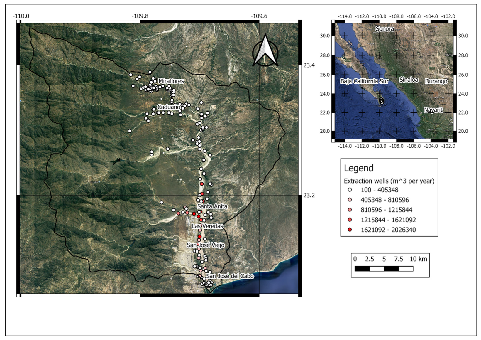
4. Social Importance and Historical Balance
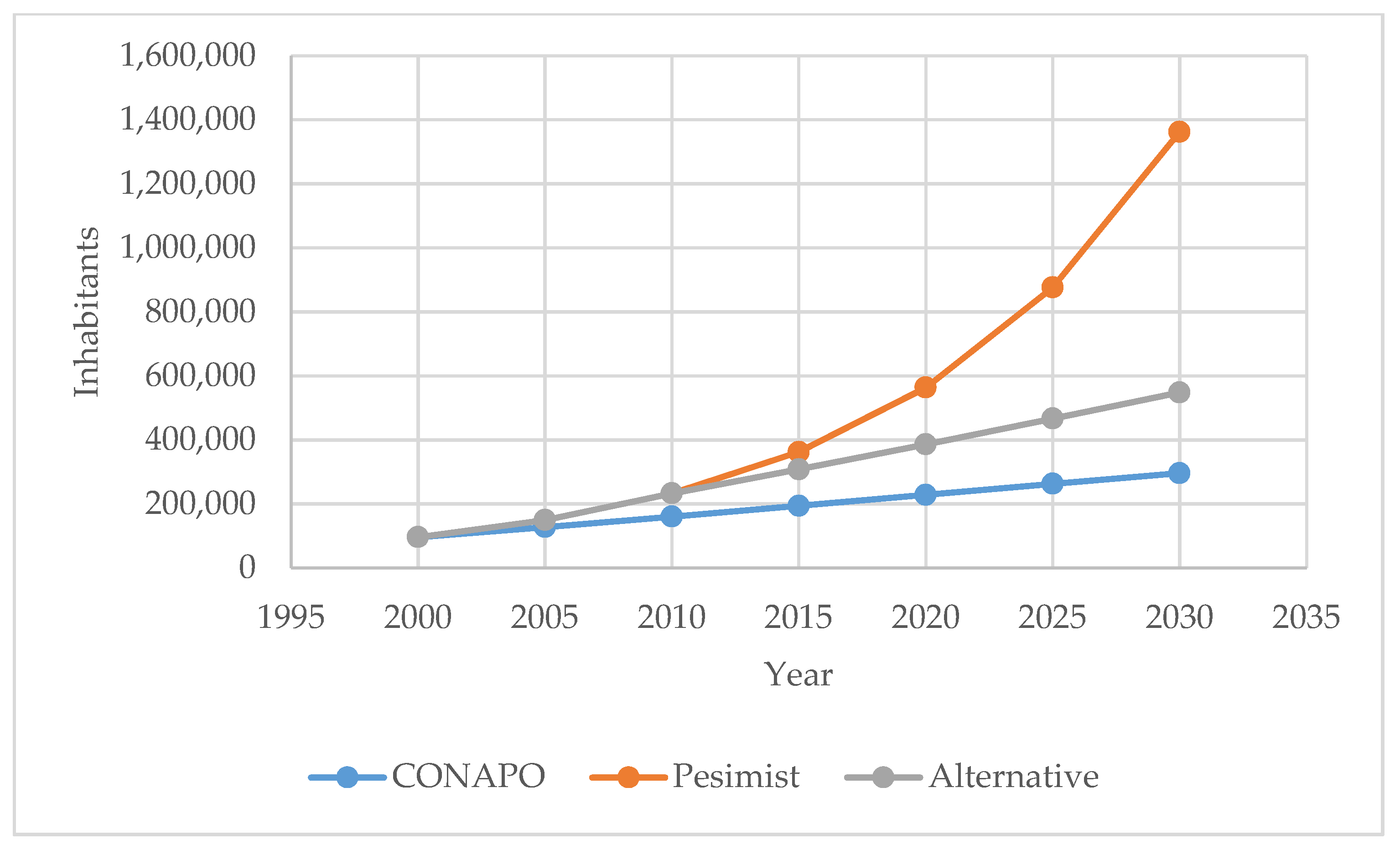
Population Growth Scenarios
5. Model Creation
- Scenario 1. Alternative extractions with recharge equal to the one registered in 2002 [8].
- Scenario 2. Alternative extractions with recharge equal to the one registered in 2011 [7].
- Scenario 3. Pessimistic extractions with recharge equal to the one registered in 2002 [8].
- Scenario 4. Pessimistic extractions with recharge equal to the one registered in 2011 [7].
- Scenario 5. Conservative extractions with recharge equal to the one registered in 2002 [8].
- Scenario 6. Conservative extractions with recharge equal to the one registered in 2011 [7].
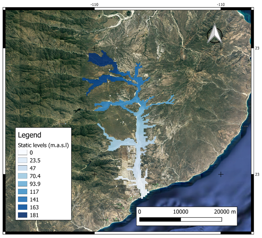
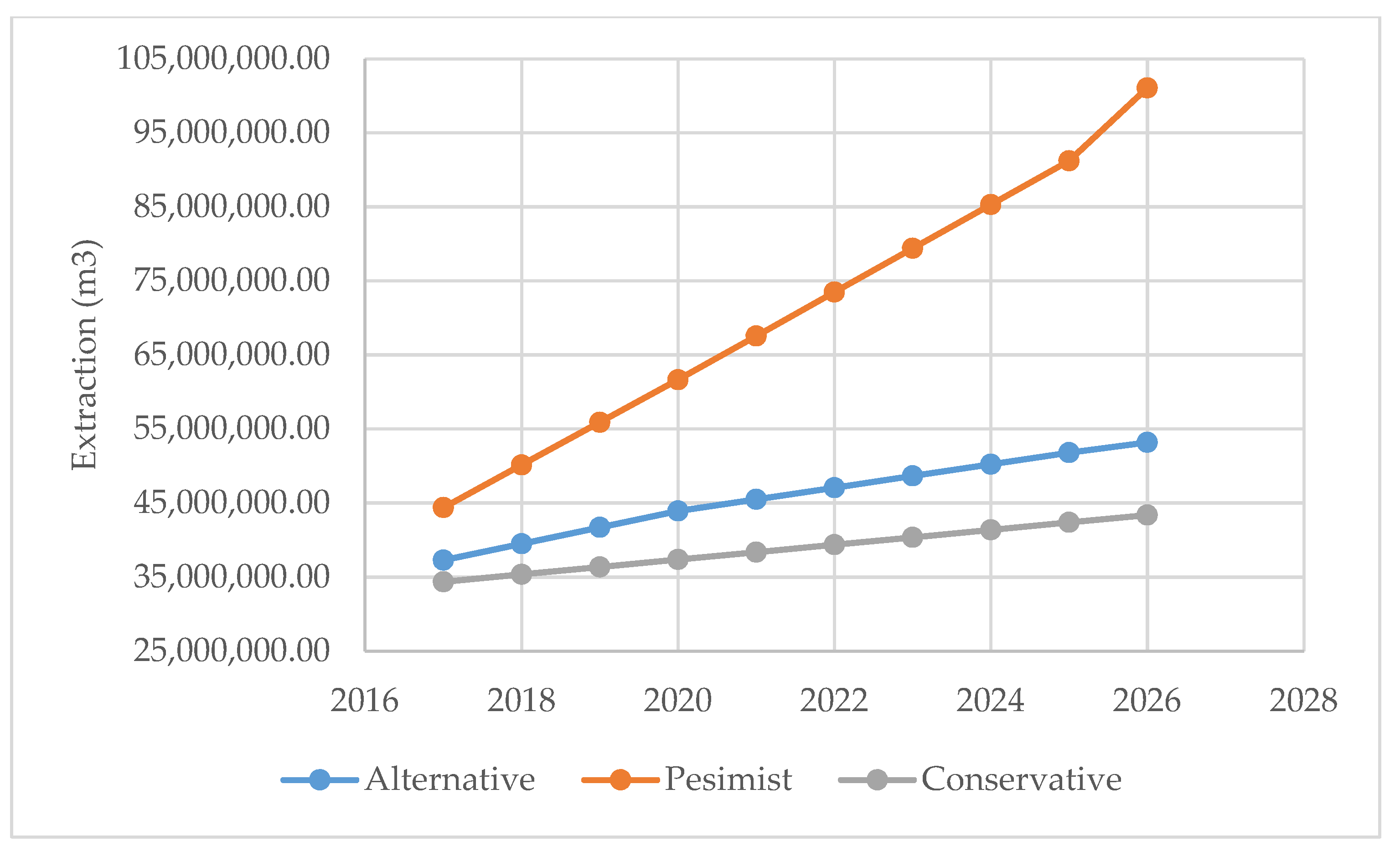
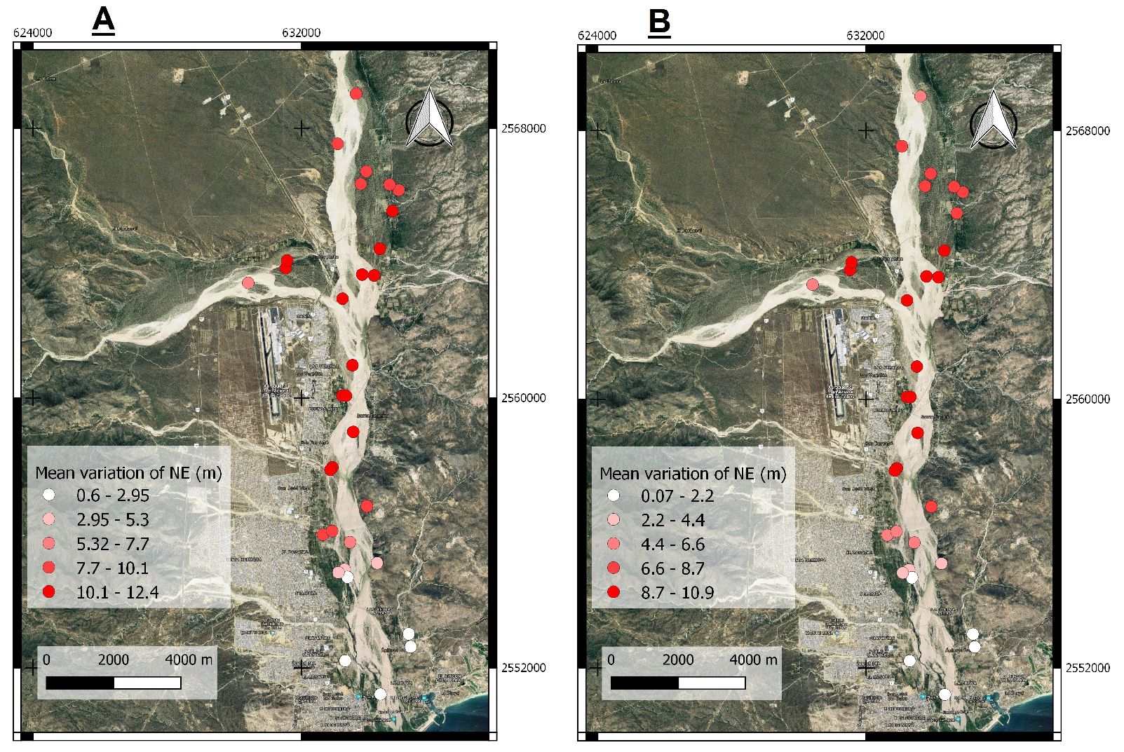
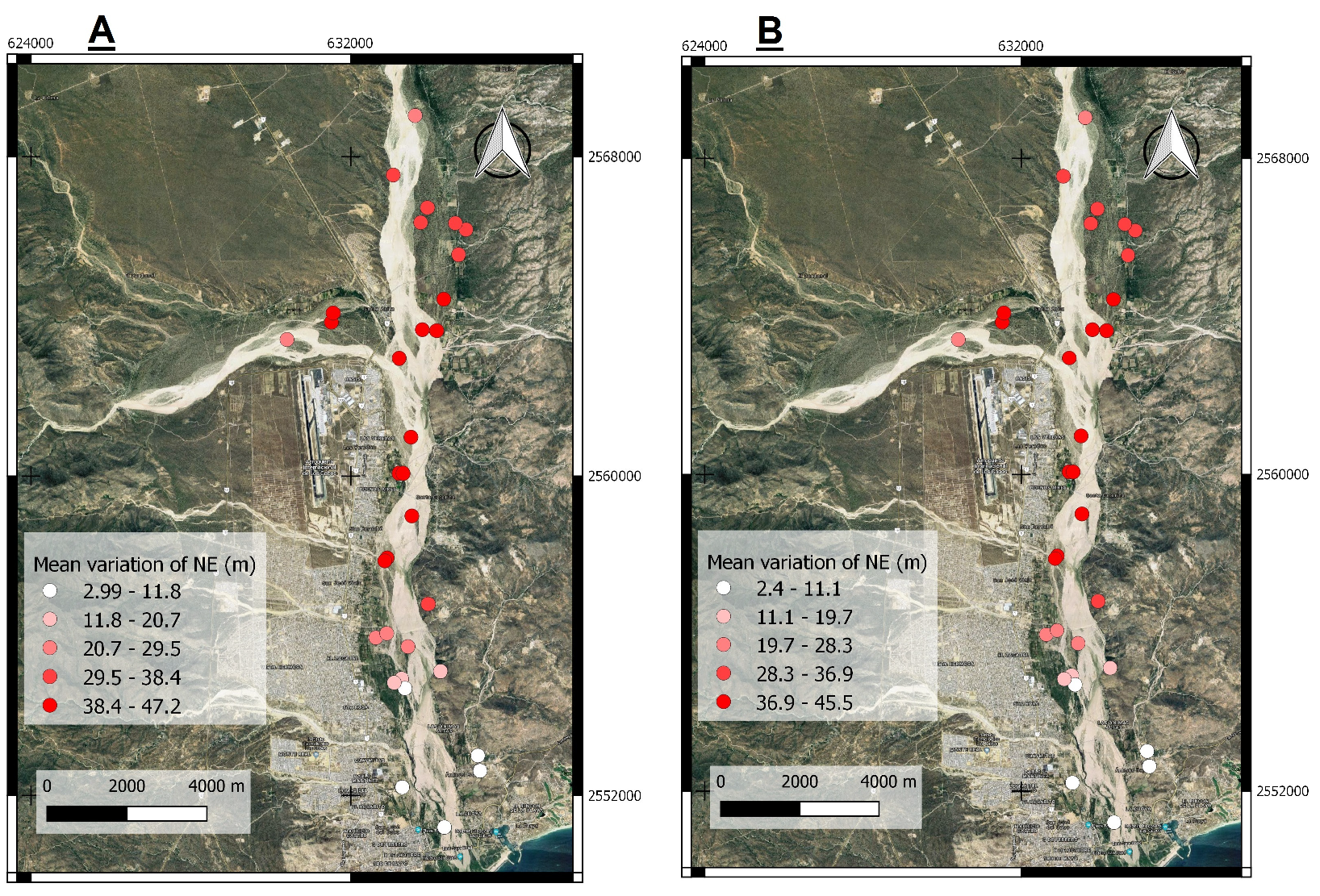
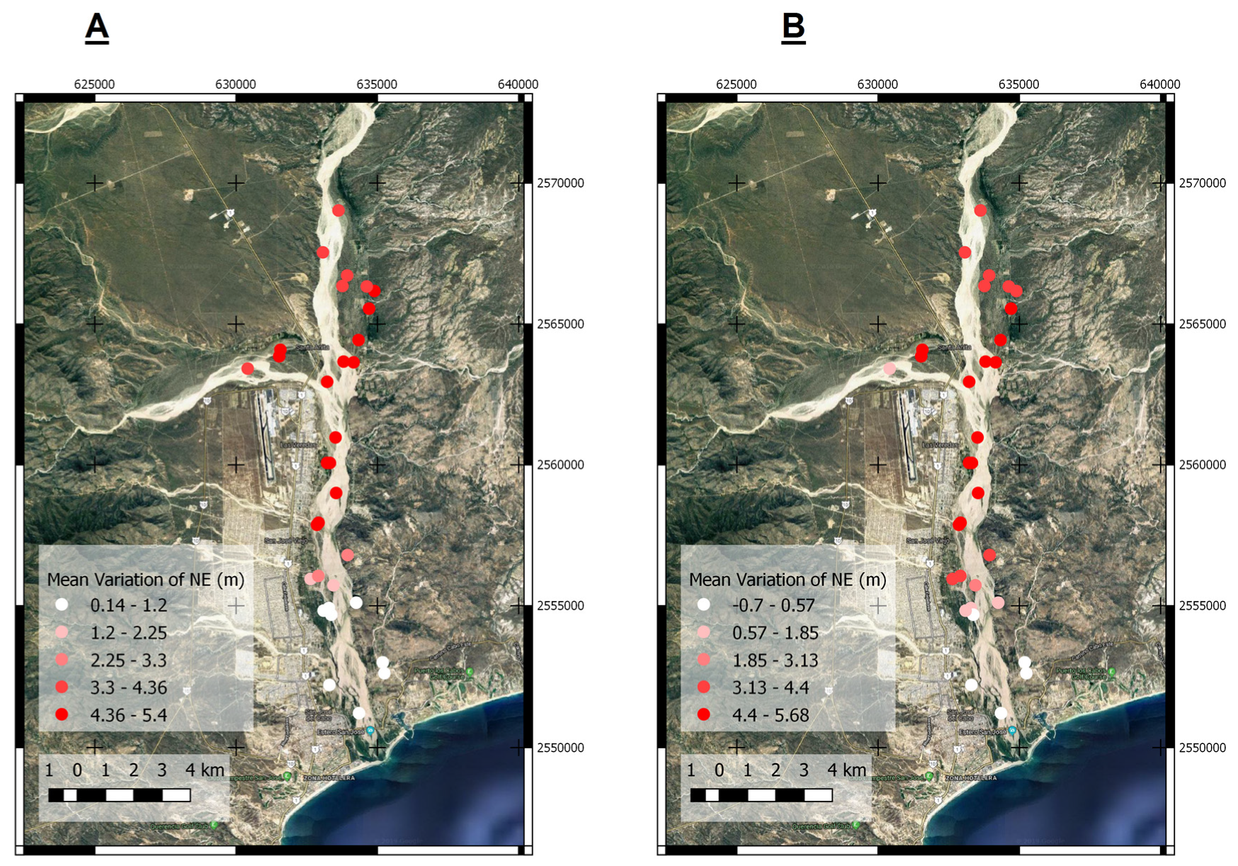
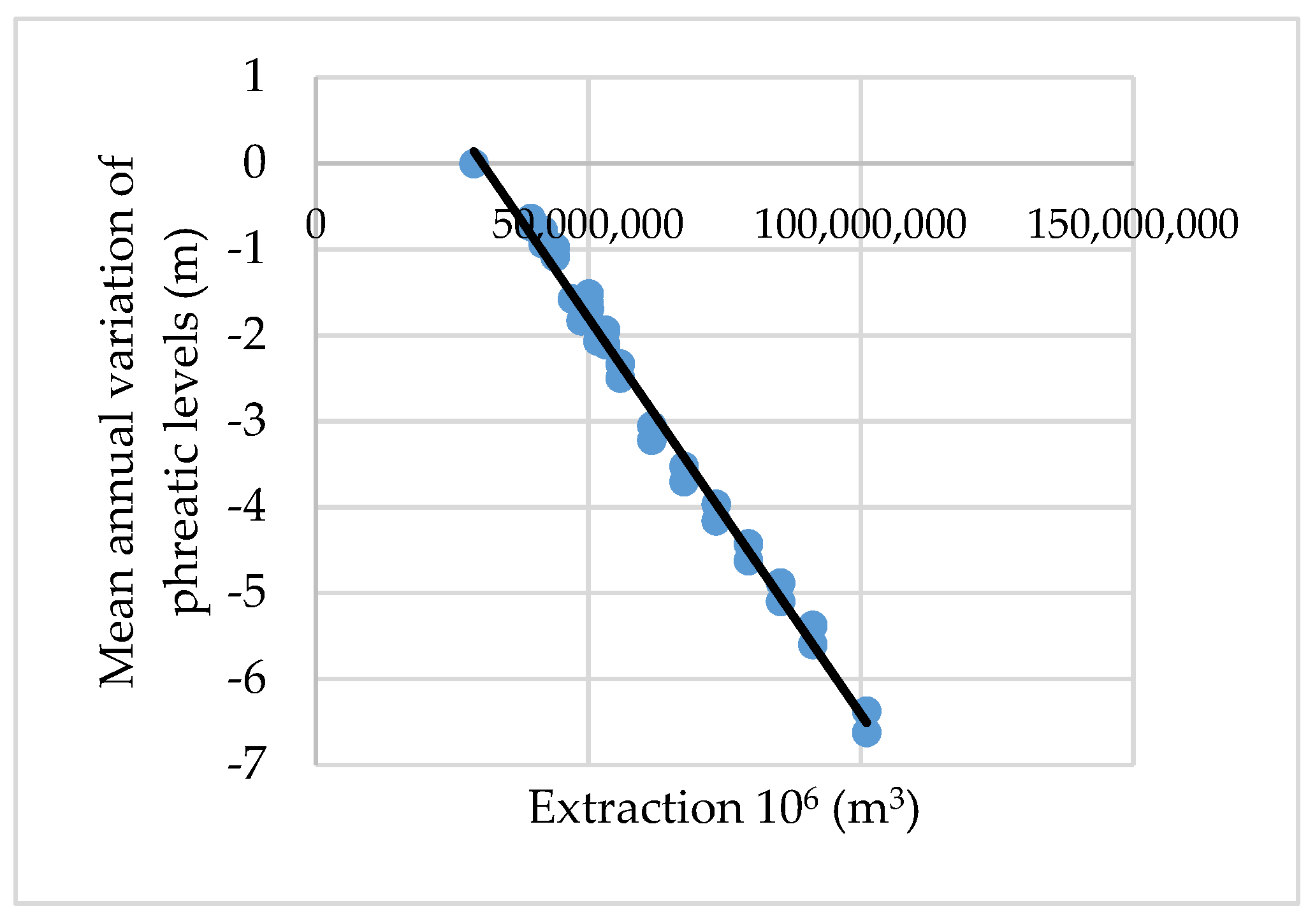
6. Results
7. Discussion
8. Conclusions
Author Contributions
Funding
Acknowledgments
Conflicts of Interest
References
- WWAP. The United Nations World Water Development Report 2015: Water for a Sustainable World, 1st ed.; UNESCO Publishing: Paris, France, 2015; Volume 1, p. 122. [Google Scholar]
- Wheater, H.S.; Mathias, S.A.; Li, X. Groundwater Modelling in Arid and Semi-Arid Areas, 1st ed.; Cambridge University Press: New York, NY, USA, 2010; p. 158. ISBN 978-0-521-11129-4. [Google Scholar]
- Weight, W.D. Hydrogeology Field Manual, 2nd ed.; McGraw-Hill: New York, NY, USA, 2008; p. 751. ISBN 0071477497. [Google Scholar]
- Merz, S.K.; Barnett, B.; Townley, L.R.; Post, V.; Evans, R.E.; Hunt, R.J.; Peeters, L.; Richardson, S.; Werner, A.D.; Knapton, A.; et al. Australian Groundwater Modelling Guidelines; Waterlines Report; National Water Commission: Camberra, Australia, 2012; ISBN 978-1-921853-91-3. [Google Scholar]
- Valdez-Aragón, A.R. Diagnóstico, Servicios Ambientales y Valoración Económica del Agua en el Corredor Turístico-Urbano de Los Cabos, BCS. Master’s Thesis, Universidad Autónoma de Baja California Sur, Baja California Sur, Mexico, 2006. (In Spanish). [Google Scholar]
- Pérez Ibáñez, R.M. Crecimiento económico, desarrollo sustentable y turismo: Una aproximación del posicionamiento de Baja California Sur (BCS) en el Barómetro de Sustentabilidad. Periplo Sustentable 2011, 20, 75–118. (In Spanish) [Google Scholar]
- CONAGUA. Actualización de la Disponibilidad Media Anual de Agua en el Acuífero San José Del Cabo (0319), Estado de Baja California Sur. 2015. Available online: https://www.gob.mx/cms/uploads/attachment/file/102821/DR_0319.pdf (accessed on 22 June 2019). (In Spanish)
- CONAGUA. Actualización de la Disponibilidad Media Anual de Agua Subterránea Acuífero (0319) San José del Cabo Estado de Baja California Sur. 2009. Available online: https://drive.google.com/open?id=1QVouI1lkNt5oHh1lIWHPRoADzhZQIwak (accessed on 22 June 2019). (In Spanish).
- Wurl, J.; Imaz Lamadrid, M.Á. Las Condiciones Hidrogeológicas en la Cuenca San José del Cabo, Baja California Sur, México. Áreas Nat. Protegidas Scr. 2016, 2, 91–102. (In Spanish) [Google Scholar] [CrossRef]
- INEGI. Memoria: XI Censo General de Población y Vivienda, 1990. Available online: http://internet.contenidos.inegi.org.mx/contenidos/Productos/prod_serv/contenidos/espanol/bvinegi/productos/historicos/2104/702825490416/702825490416_1.pdf (accessed on 22 June 2019). (In Spanish).
- INEGI. Memoria del Conteo de Población y Vivienda 1995. Available online: http://internet.contenidos.inegi.org.mx/contenidos/Productos/prod_serv/contenidos/espanol/bvinegi/productos/metodologias/est/702825000746.pdf (accessed on 22 June 2019). (In Spanish).
- INEGI. Memoria XII Censo General de Población y Vivienda 2000. Available online: http://internet.contenidos.inegi.org.mx/contenidos/Productos/prod_serv/contenidos/espanol/bvinegi/productos/historicos/1329/702825006519/702825006519_1.pdf (accessed on 22 June 2019). (In Spanish).
- INEGI. Censo General de Población y Vivienda 2010. Available online: http://internet.contenidos.inegi.org.mx/contenidos/productos/prod_serv/contenidos/espanol/bvinegi/productos/censos/poblacion/2010/perfil_socio/uem/702825047610_1.pdf (accessed on 22 June 2019). (In Spanish).
- INEGI. Tabulados de Encuesta Intercensal 2015. Available online: http://www.coespo.sonora.gob.mx/indicadores/sociodemograficos/tabulados-de-la-encuesta-intercensal-2015-inegi.html (accessed on 22 June 2019). (In Spanish)
- CONAGUA. Información Climatológica. Available online: http://smn.cna.gob.mx/es/climatologia/informacion-climatologica (accessed on 5 June 2019). (In Spanish)
- Martínez Gutiérrez, G.M.; Díaz Gutiérrez, J.J.; Cosío González, O.G. Geología. Informe final. In Programa de Manejo para la Cuenca Hidrológica-Forestal San José del Cabo, B.C.S.; Center for Biological Research of the Northwest, S.C. (CIBNOR): Baja California Sur, Mexico, 2007; pp. 1–40. ISBN 9701307976. (In Spanish) [Google Scholar]
- Valdez-Aragón, A.; Breceda, A.; Pombo, A. Capítulo 8 Diagnostico del Uso del Agua. In Programa de Manejo para Cuenca Hidrológica-Forestal San José del Cabo, B. C. S.; CIBNOR-UABCS: Baja California Sur, Mexico, 2002; pp. 314–387. (In Spanish) [Google Scholar]
- Wurl, J.; Valdez-Aragón, A.R. Clima. Informe Final. In Programa de Manejo para Cuenca Hidrológica-Forestal San José del Cabo, B. C. S; CONAFOR-2002-C01-5671; CIBNOR-UABCS: Baja California Sur, Mexico, 2007; pp. 46–56. (In Spanish) [Google Scholar]
- Imaz-Lamadrid, M.A.; Wurl, J.; Ramos-Velázquez, E. Future of coastal lagoons in arid zones under climate change and anthropogenic pressure. A case study from San Jose Lagoon, Mexico. Resources 2019, 8, 57. [Google Scholar] [CrossRef]
- Harbaugh, A.W. MODFLOW-2005, the US Geological Survey Modular Ground-Water Model: The Ground-Water Flow Process; US Department of the Interior, US Geological Survey: Reston, VA, USA, 2005.
- Winston, R.B. ModelMuse: A Graphical User Interface for MODFLOW-2005 and PHAST; US Geological Survey: Reston, VA, USA, 2009.
- García, E. Modificaciones al Sistema de Clasificación Climática de Köeppen (para Adaptarlo a las Condiciones de la República Mexicana); Instituto de Geografía Universidad Nacional Autónoma de México: México City, Mexico, 1973. (In Spanish) [Google Scholar]
- Maderey-Rascón, L.E. Mapa de Evapotranspiración Real, Escala: 1:4,000,000. Available online: http://www.conabio.gob.mx/informacion/gis/?vns=gis_root/clima/evapot/evaprv4mgw (accessed on 22 June 2019). (In Spanish)
- Wurl, J.; Hernández Morales, P.; Gaytán García, J.; Martínez Meza, J.E.; Imaz Lamadrid, M.A. Hidrogeológia. Informe final. In Programa de Manejo para Cuenca Hidrológica-Forestal San José del Cabo, B. C. S.; Center for Biological Research of the Northwest, S.C. (CIBNOR): Baja California Sur, Mexico, 2002; pp. 69–159. (In Spanish) [Google Scholar]
- Strahler, A.N. Quantitative analysis of watershed geomorphology. Trans. Am. Geophys. Union 1957, 38, 913–920. [Google Scholar] [CrossRef]
- Maya, Y.; Marín, B.; Argueta, A. Capítulo 5 Suelos y erosión. In Programa de Manejo para Cuenca Hidrológica-Forestal San José del Cabo, B. C. S.; CIBNOR-UABCS: Baja California Sur, Mexico, 2002; pp. 160–174. (In Spanish) [Google Scholar]
- Stock, J.M.; Hodges, K.V. Pre-Pliocene extension around the Gulf of California and the transfer of Baja California to the Pacific plate. Tectonics 1989, 8, 99–115. [Google Scholar] [CrossRef]
- Martinez-Gutierrez, G.; Sethi, P.S. Miocene-Pleistocene sediments within the San Jose del Cabo Basin, Baja California Sur, Mexico. Spec. Pap. Geol. Soc. Am. 1997, 318, 141–166. [Google Scholar]
- Piña-Arce, M. Bioestratigrafía con Nanofósiles Calcáreos en el Área Los Algodones, B. C. S. Ph.D. Thesis, Universidad Autónoma de Baja California Sur, Baja California Sur, Mexico, 2010. (In Spanish). [Google Scholar]
- Busch, M.M.; Arrowsmith, J.R.; Umhoefer, P.J.; Coyan, J.A.; Maloney, S.J.; Gutierrez, G.M. Geometry and evolution of rift-margin, normal-fault-bounded basins from gravity and geology, La Paz-Los Cabos region, Baja California Sur, Mexico. Lithosphere 2011, 3, 110–127. [Google Scholar] [CrossRef]
- Arreguín-Rodríguez, G.D.J.; Schwennicke, T. Estratigrafía de la margen occidental de la cuenca San José del Cabo, Baja California Sur. Boletín Soc. Geológica Mex. 2013, 65, 481–496. (In Spanish) [Google Scholar] [CrossRef]
- Benton y Asesores, S.C. Estudio y Diseño de Captaciones y Conducciones a los Acueductos Existentes en el Valle de San José del Cabo y el Corredor Entre Esta Población y Cabo San Lucas. Cabo Baja California Sur; National Water Commission: México City, Mexico, 1998; 322p. (In Spanish) [Google Scholar]
- INEGI. Zona Hidrogeológica San José del Cabo, Escala 1:150,000; Instituto Nacional de Estadística y Geografía: México City, Mexico, 2013. (In Spanish)
- SARH. Resultados de las Pruebas de Bombeo, Zona del Valle de San José del Cabo, Baja California Sur, Escala 1: 50,000; Secretaría de Agricultura y Recursos Hidráulicos: México City, Mexico, 1979. (In Spanish) [Google Scholar]
- INEGI. Conteo de Población y Vivienda 2005. Indicadores del Censo Gen. Población y Vivienda, México; Instituto Nacional de Estadística y Geografía: México City, Mexico, 2005. (In Spanish)
- Middlemis, H. Groundwater Flow Modelling Guideline; Murray-Darling Basin Commission: South Pert, Australia, 2001; p. 133.
- Kumar, C.P. Modelling of groundwater flow and data requirements. Int. J. Mod. Sci. Eng. Technol. 2015, 2, 18–27. [Google Scholar]
- Martínez-Gutiérrez, G.; Díaz, J.J. Morfometría en la cuenca hidrológica de San José del Cabo, Baja California Sur, México. Rev. Geogr. Am. Cent. 2011, 44, 83–100. (In Spanish) [Google Scholar]
- CONAGUA. Registro Público de Derechos de Agua (REPDA). Available online: https://app.conagua.gob.mx/Repda.aspx (accessed on 24 June 2019). (In Spanish)
- R Core Team. R: A Language and Environment for Statistical Computing; R Core Team: Viena, Austria, 2018. [Google Scholar]
- Heath, R. Basic Ground-Water Hydrology; USGS Publications Warehouse: Washington, DC, USA, 1983; Volume 2220.
- Morris, D.A.; Johnson, A.I. Summary of Hydrological and Physical Properties of Rock and Soils Material; USGS Publications Warehouse: Washington, DC, USA, 1967.
- Bear, J. Dynamics of Fluids in Porous Media; American Elsevier Publishing Company, Inc.: New York, NY, USA, 1972. [Google Scholar]
- SEA. Guía para el uso de Modelos de Aguas Subterráneas en el SEIA; SEA (Servicio de Evaluación Ambiental): Santiago de Chile, Chile, 2012. (In Spanish)
- Kumar, C.P. Basic Guidelines for Groundwater Modelling Studies. ISH J. Hydraul. Eng. 2003, 9, 11–21. [Google Scholar] [CrossRef]
- Reilly, T.E.; Harbaugh, A.W. Guidelines for Evaluating Ground-Water Flow Models; US Department of the Interior, US Geological Survey: Reston, VA, USA, 2004.
- Wels, C.; Mackie, D.; Scibek, J. Guidelines for Groundwater Modelling to Assess Impacts of Proposed Natural Resource Development Activities; Ministry of Environment, Water Protection & Sustainability Branch: British Columbia, BC, Canada, 2012.
- Sahoo, S.; Jha, M.K. On the statistical forecasting of groundwater levels in unconfined aquifer systems. Environ. Earth Sci. 2015, 73, 3119–3136. [Google Scholar] [CrossRef]
- Bulla-cruz, L.A.; Ruge, J.C. Assessment of groundwater level variations using multivariate statistical methods. Ing. Investig. 2019, 39, 1–7. [Google Scholar]
- Cruz Falcón, A.; Ramírez-Hernández, J.; Vázquez-González, R.; Nava-Sánchez, E.H.; Troyo-Diéguez, E.; Fraga-Palomino, H.C. Estimación de la Recarga y Balance Hidrológico del Acuífero de La Paz, BCS, México, Universidad y Ciencia. Available online: http://www.redalyc.org/articulo.oa?id=15426919007 (accessed on 22 June 2019). (In Spanish).
- Wurl, J.; Imaz-Lamadrid, M.A. Coupled surface water and groundwater model to design managed aquifer Coupled surface water and groundwater model to design managed aquifer recharge for the valley of Santo Domingo, B.C.S., Mexico. Sustain. Water Resour. Manag. 2017, 4, 361–369. [Google Scholar] [CrossRef]
- Suryanarayana, C.; Mahammood, V. Groundwater-level assessment and prediction using realistic pumping and recharge rates for semi-arid coastal regions: A case study of Visakhapatnam city, India. Hydrogeol. J. 2019, 27, 249–272. [Google Scholar] [CrossRef]
- Rozman, D.; Hrkal, Z.; Tesař, M. Artificial recharge of a shallow hard rock aquifer as a climate change mitigation method: Model solution from the Czech Republic. Model. Earth Syst. Environ. 2019, 5, 605–612. [Google Scholar] [CrossRef]
- Chunn, D.; Faramarzi, M.; Smerdon, B.; Alessi, D.S. Application of an Integrated SWAT—MODFLOW Model to Evaluate Potential Impacts of Climate Change and Water Withdrawals on Groundwater—Surface Water Interactions in West-Central Alberta. Water 2019, 11, 110. [Google Scholar] [CrossRef]
- Zhu, J.; Wang, Y.; Guo, H.; Zang, X.; Qin, T. Application of Groundwater Model to Groundwater Regulation in Cangzhou Area. E3S Web Conf. 2019, 79, 03014. [Google Scholar] [CrossRef]


| Unit | Hydraulic Conductivity (ms−1) | Specific Storage (%) | Specific Yield (%) | Thickness (m) |
|---|---|---|---|---|
| A | 0.007 to 0.00005 | 3 | 15 to 20 | 500 to 50 |
| B | 1 × 10⁻⁶ | 0.08 | 0.09 | 180~280 |
| C | 12 × 10−12 | 0.01 | 0.09 | 100 |
| R | Ind. R | DIS | EVT | Wells | In | Out | Balance | Mid | Low | |
|---|---|---|---|---|---|---|---|---|---|---|
| E1.-2017 | 24 | 1.50 | 3.48 | 1.10 | 37.28 | 25.50 | 41.86 | −16.36 | ||
| E1.-2026 | 24 | 1.50 | 3.24 | 1.10 | 53.18 | 25.50 | 57.52 | −32.02 | −10.49 | −2.20 |
| E2.-2017 | 30 | 1.50 | 3.59 | 1.10 | 37.28 | 31.50 | 41.96 | −10.46 | ||
| E2.-2026 | 30 | 1.50 | 3.56 | 1.10 | 53.18 | 31.50 | 57.85 | −26.35 | −9.07 | −1.50 |
| E3.-2017 | 24 | 1.50 | 3.45 | 1.10 | 44.37 | 25.50 | 48.93 | −23.43 | ||
| E3.-2026 | 24 | 1.50 | 2.26 | 1.10 | 101.08 | 25.50 | 104.44 | −78.94 | −37.16 | −8.80 |
| E4.-2017 | 30 | 1.50 | 3.59 | 1.10 | 44.37 | 31.50 | 49.06 | −17.56 | ||
| E4.-2026 | 30 | 1.50 | 2.61 | 1.10 | 101.08 | 31.50 | 104.79 | −73.29 | −35.47 | −8.10 |
| E5.-2017 | 24 | 1.50 | 3.40 | 1.10 | 34.35 | 25.50 | 38.85 | −13.35 | ||
| E5.-2026 | 24 | 1.50 | 3.23 | 1.10 | 43.37 | 25.50 | 47.87 | −22.37 | −4.53 | −1.78 |
| E6.-2017 | 30 | 1.50 | 3.60 | 1.10 | 34.35 | 31.50 | 39.05 | −7.55 | ||
| E6.-2026 | 30 | 1.50 | 3.55 | 1.10 | 43.37 | 31.50 | 48.12 | −16.62 | −4.24 | −1.37 |
| Parameters | B | SE | t | p-Level | Cor. Pearson | |
|---|---|---|---|---|---|---|
| A | ||||||
| Int | 3.2 | 2.57 × 10+5 | 12.435 | 7.81 × 10⁻¹⁶ | ||
| Ext | −1.21 × 10⁻² | 1.231.61 × 10−3 | −9.795 | 1.61 × 10⁻¹² | ||
| Re | 2.83 × 10⁻² | 8.29 × 10⁻³ | 3.41 | 0.00142 | ||
| B | ||||||
| Int | 2.23 | 2.22 × 10⁻¹ | 10.079 | 6.79 × 10⁻¹³ | ||
| Ext | −9.17 × 10⁻⁸ | 1.06 × 10⁻⁹ | −86.319 | 2.00 × 10⁻¹⁶ | ||
| Re | 1.92 × 10⁻⁸ | 7.14 × 10⁻⁹ | 2.689 | 0.0102 | ||
| C | ||||||
| Int | 1.03 | 2.67 × 10⁻¹ | 3.856 | 0.000372 | ||
| Ext | −2.77 × 10⁻⁸ | 1.24 × 10⁻⁹ | −22.367 | 2.00 × 10⁻¹⁶ | ||
| Re | 1.27 × 10⁻⁹ | 8.70 × 10⁻⁹ | 0.146 | 0.884 | ||
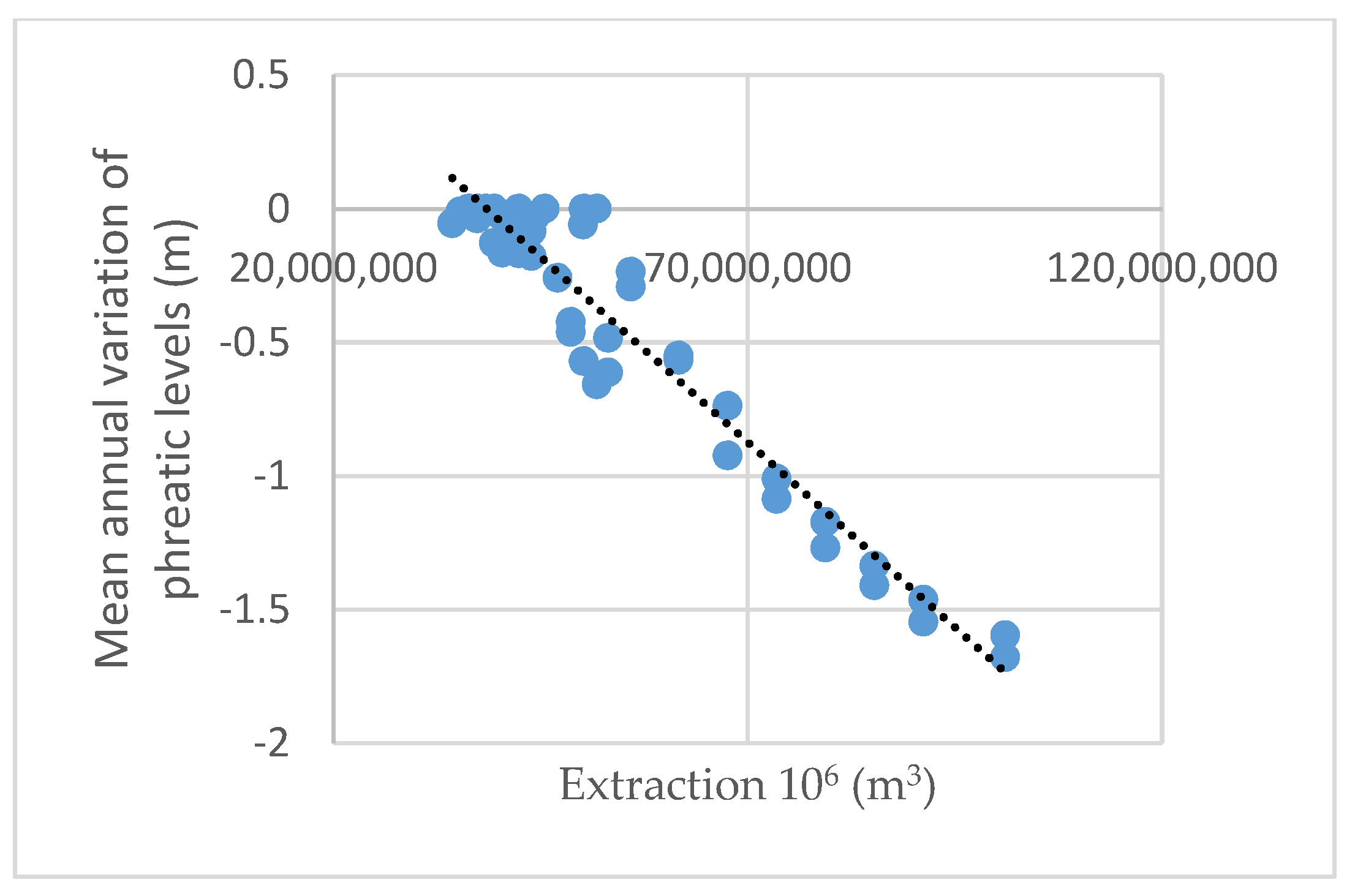
| Regression Equation A | df = 3.2 − 0.01209 x ext + 0.02827 x re | 0.857 | ||||
| Regression Equation B | df = 2.233 − 9.17 × 10⁻⁸ x ext + 1.92 × 10⁻⁸ x re | 0.997 | ||||
| Regression Equation C | df = 1.029 − 2.77 × 10⁻⁸ x ext + 1.27 × 10⁻⁹ x re | 0.963 | ||||
© 2019 by the authors. Licensee MDPI, Basel, Switzerland. This article is an open access article distributed under the terms and conditions of the Creative Commons Attribution (CC BY) license (http://creativecommons.org/licenses/by/4.0/).
Share and Cite
Trasviña-Carrillo, J.A.; Wurl, J.; Imaz-Lamadrid, M.A. Groundwater Flow Model and Statistical Comparisons Used in Sustainability of Aquifers in Arid Regions. Resources 2019, 8, 134. https://doi.org/10.3390/resources8030134
Trasviña-Carrillo JA, Wurl J, Imaz-Lamadrid MA. Groundwater Flow Model and Statistical Comparisons Used in Sustainability of Aquifers in Arid Regions. Resources. 2019; 8(3):134. https://doi.org/10.3390/resources8030134
Chicago/Turabian StyleTrasviña-Carrillo, Javier Alexis, Jobst Wurl, and Miguel Angel Imaz-Lamadrid. 2019. "Groundwater Flow Model and Statistical Comparisons Used in Sustainability of Aquifers in Arid Regions" Resources 8, no. 3: 134. https://doi.org/10.3390/resources8030134