AMC2N: Automatic Modulation Classification Using Feature Clustering-Based Two-Lane Capsule Networks

Abstract

The automatic modulation classification (AMC) of a detected signal has gained considerable prominence in recent years owing to its numerous facilities. Numerous studies have focused on feature-based AMC. However, improving accuracy under low signal-to-noise ratio (SNR) rates is a serious issue in AMC. Moreover, research on the enhancement of AMC performance under low and high SNR rates is limited. Motivated by these issues, this study proposes AMC using a feature clustering-based two-lane capsule network (AMC2N). In the AMC2N, accuracy of the MC process is improved by designing a new two-layer capsule network (TL-CapsNet), and classification time is reduced by introducing a new feature clustering approach in the TL-CapsNet. Firstly, the AMC2N executes blind equalization, sampling, and quantization in trilevel preprocessing. Blind equalization is executed using a binary constant modulus algorithm to avoid intersymbol interference. To extract features from the preprocessed signal and classify signals accurately, the AMC2N employs the TL-CapsNet, in which individual lanes are incorporated to process the real and imaginary parts of the signal. In addition, it is robust to SNR variations, that is, low and high SNR rates. The TL-CapsNet extracts features from the real and imaginary parts of the given signal, which are then clustered based on feature similarity. For feature extraction and clustering, the dynamic routing procedure of the TL-CapsNet is adopted. Finally, classification is performed in the SoftMax layer of the TL-CapsNet. This study proves that the AMC2N outperforms existing methods, particularly, convolutional neural network(CNN), Robust-CNN (R-CNN), curriculum learning(CL), and Local Binary Pattern (LBP), in terms of accuracy, precision, recall, F-score, and computation time. All metrics are validated in two scenarios, and the proposed method shows promising results in both.

1. Introduction

In wireless communication, the contribution of automatic modulation classification (AMC) has grown dramatically because of its convenience in a wide range of applications [1]. The AMC technique reduces the overhead caused by sharing modulation scheme between transmitter and receiver [2]. For example, many military applications demand automatic detection of modulation schemes utilized by the signal from adversaries [3,4]. This type of application also incorporates signal jamming and interception. As a result, AMC plays an essential role in civilian and military applications regarding the recognition of received signals. For instance, digital modulation classification (MC) methods have had a paradigm shift from manual operational systems to automatic systems because of their several advantages. Manual modulation clarification (MMC) requires manual measurement of parameters of intercepted signals to recognize modulation types. In MMC, four types of information, namely, intermediate frequency time waveform, average and instantaneous spectra of signal, sound and signal, and instantaneous amplitude, are available for the search operator. Manual analysis becomes problematic and inaccurate when the number of intercepted modulation types increases. This method also requires experienced analyzers and does not guarantee reliable classification results. However, these shortcomings can be addressed via AMC. AMC is more powerful than MMC because it integrates an automatic modulation recognizer into an electronic receiver.

In prior works, two traditional processes have been executed to identify the modulation type of the received signal [5,6,7]. They are maximum likelihood- and feature extraction-based modulation identification. The maximum likelihood-based classification method executes the likelihood function on the received signal [8]. Examples of systems that use this approach are (i) faster maximum likelihood function-based MC [9], (ii) expectation conditional maximization algorithm [10], and (iii) sparse coefficient-based expectation maximization algorithm [11].

Although the maximum likelihood-based classification method provides an optimal solution in AMC, it suffers from substantial computational complexity issues. It also demands the prior information of the transmitter. On the contrary, the feature-based AMC (FB-AMC) method has less computation time and does not require prior information about the transmitter. It relies on two significant processes, namely, feature extraction and classification [7]. The higher-order statistics (HOS) features present in the time domain were considered by authors in [12,13] for MC. The authors in [14] introduced compressive sensing aided FB-AMC, in which the cyclic feature was extracted to classify the modulation type of the signal.

Machine learning (ML)-based feature classification methods such as support vector machine (SVM), K-nearest neighbor (KNN), neural networks, and so on have been studied in many preceding papers associated with AMC. The authors in [15] utilized the long short-term memory (LSTM) algorithm to classify the modulation type of the given signal. The deep hierarchical network-based algorithm was exploited in [16] to perform effective MC. The extreme learning machine algorithm was utilized to classify the modulation type of the given signal in [17]. Reference [18] used a linear discriminant analysis (LDA) classifier to detect the accurate modulation type of the signal acquired from the transmitter.

From the detailed literature review (discussed in Section 2), it can be seen that FB-AMC still faces drawbacks in the detection of accurate modulation type of the given signal. The reasons are as follows:

• Significant preprocessing steps, such as blind equalization and sampling, are not considered before MC.
• The lack of consideration of significant features, such as time and frequency, during the feature extraction process leads to a reduction in accuracy in feature extraction and classification.
• Most FB-AMC methods cannot achieve high accuracy at low signal-to-noise ratio (SNR) rate due to the lack of concentration in enhancing the performance of ML-based classification algorithms.

AMC has gained much interest owing to its wide range of applications, such as electronic surveillance and electromagnetic signal monitoring. Nevertheless, it faces many difficulties during modulation detection [19] because it does not utilize any prior knowledge, such as channel state information, signal-to-noise ratio (SNR), and noise characteristics. In the literature, many works have concentrated on feature-based MC. However, they did not consider effective preprocessing mechanisms to enhance the quality of the received signal [20]. Likewise, ML-based feature extraction and classification have been exploited in many AMC-related works. Still, they are insufficient in enhancing accuracy in high and low SNR rates. Furthermore, ML-based algorithms introduce complexity into MC [21]. Here, the machine learning algorithm uses high-order cumulant features with standard decision criteria. This issue has been resolved by a few works in FB-AMC. To address these downsides in current AMC studies, a new AMC, called AMC by using two-layer capsule network (TL-CapsNet) (AMC2N), is proposed. It has the following objectives:

• To increase the quality of the received signal, before the MC process;
• To increase the accuracy in feature extraction, even at a low SNR rate;
• To enhance the performance of ML-based MC;
• To enhance the accuracy, during classification for low and high SNR rates.

To achieve improved performance in MC, our AMC2N method contributes the following processes:

• This work presents a novel TL-CapsNet model for the accurate classification of modulation schemes. The proposed TL-CapsNet differs from existing works by analyzing the real and imaginary parts of received signals.
• Firstly, the AMC2N enhances received signal quality using a trilevel preprocessing method. This work executes three processes, namely, blind equalization, sampling, and quantization. The binary constant modulus algorithm (BCMA) is employed for the blind equalization, which evades the intersymbol interference (ISI) of the signal. Furthermore, sampling and quantization are performed to reduce aliasing effects and the bits necessary to represent the given signal. This proposed preprocessing method can enhance AMC accuracy.
• Secondly, a novel TL-CapsNet is introduced to process the preprocessed signal. The TL-CapsNet has three major responsibilities, i.e., (i) feature extraction, in which the TL-CapsNet extracts all important features from the real and imaginary parts of the signal in parallel; (ii) feature clustering, in which all extracted features are clustered based on feature similarity factors in the TL-CapsNet to boost the classification process; and (iii) modulation classification.

Finally, the performance of the AMC2N method is evaluated using five validation metrics, including accuracy, precision, recall, F-Score, and computation time. The simulation results are compared with those of existing methods.

The rest of this paper is organized as follows: In Section 2, we review prior works related to FB-AMC; in Section 3, we provide a signal model of the proposed AMC2N method; in Section 4, we explain the proposed AMC2N method with the proposed algorithms; in Section 5, we elucidate the experimental evaluation of the proposed AMC2N method; and in Section 6, we conclude the contribution of this study and discusses future directions.

2. State-of-the-Art Methods

This section reviews state-of-the-art works associated with FB-AMC. AMC systems are generally divided into two groups. The first group is AMC without ML, in which features are not extracted using ML techniques. The second group is AMC with ML, in which features are extracted using ML techniques.

2.1. Automatic Modulation Classification (AMC) without Machine Learning (ML)

Ali et al. [22] applied principal component analysis (PCA) to the modulation scheme classification of phase shift keying (PSK), frequency shift keying (FSK), and quadrature amplitude modulation (QAM). The PCA method was used to extract features from the received signal. Then, the feature vector from the PCA method was directly provided to k-nearest neighbour (k-NN) and SVM classifiers. Features were generated by utilizing the distinct characteristics of modulated signals in the ambiguity domain to classify the modulation scheme of the given signal. The data used were at values of SNR equal to −4 dB and 16 dB. Classification mean accuracy of 80% was achieved at −4 dB to 16 dB SNR range. Nonetheless, PCA has the issue of information loss, and thus degrades the AMC performance. Kosmowski et al. [23] introduced the average likelihood ratio test (ALRT)-based AMC approach. A cumulant-based approach was exploited to extract features, in which higher-order cumulant features were utilized in MC. On the basis of these features, the modulation scheme of the received signal was obtained. During simulation, this method achieved mean accuracy of 75% at −5 dB to 20 dB. However, the probability of correct classification (PCC) still needed high SNR to obtain high PCC, and this method required a complex computation process.

A feature weighting (FW) method-based AMC was proposed by Daldal et al. [24]. Twelve time-domain features and four frequency-domain features were extracted from the received signal. Then, the features were fed into neutrosophic c-means (NCM) clustering to provide weights to each feature. The weighted features were considered for the MC process. Five classifiers, namely, LDA, SVM, k-NN, AdaBoostM1, and random forest, were analyzed to detect the optimal modulation scheme of the given signal. This study achieved a mean of 83% in precision and recall and a mean of 88% in accuracy at 0 to 25 dB SNR rate. Random forest was determined to be the best classifier for AMC. Nevertheless, this method needed a complex computational process for constructing a decision tree, which was highly difficult when the number of features increased. Daldal et al. [25] contributed to the determination of modulation scheme by using time and frequency-based information. The short-term Fourier transform (STFT) algorithm was utilized to extract features from the given signal, whilst the CNN algorithm was utilized to classify the extracted features. The proposed method successfully achieved mean accuracy of 92% at 0 to 25 dB. However, this method lacked an effective preprocessing mechanism, such as blind equalization and quantization, which led to slow processing. This problem was due to the difficulties introduced (such as intersymbol interference (ISI) and infinite values) during the feature extraction process. Zhang et al. [26] introduced the modulation detection scheme M-QAM with the aid of the adaptive fuzzy clustering (AFC) model. Preprocessing was performed before feature extraction. Then, features extracted were clustered using the AFC model. From the clustered result, the modulation type of the given signal was finally classified. The proposed method showed high accuracy of 93% at high SNR rate, i.e., 20 dB, but produced ineffective results under low SNR rate, i.e., −10 dB.

Li et al. [27] introduced the FB-AMC approach. Two types of feature sets, namely, statistical and spectral features, were considered for modulation detection. Then, these feature sets were processed into the SVM classifier to detect the modulation type of the received signal. The result showed good recognition at low SNR with accuracy up to 90%. Nonetheless, this method required a complex computation process due to the lack of capability in handling large datasets in the SVM classifier. In another research, the cyclic correntopy spectrum-based MC approach was introduced by Ma et al. [28]. Cycle frequencies (CF) were utilized to classify the modulation type of the signal. These features were processed via PCA before the modulation detection process. In the proposed research, a radial basis function (RBF)-based neural network was utilized to classify the modulation type of the given signal. It achieved high accuracy above 90% at −5 dB to 10 dB SNR rate. However, CF required a complex computation process and resulted in slow processing for classification. In addition, the proposed method was not robust at low SNR because of the slow performance of the RBF-based neural network, given that every node in the hidden layer needed to compute RBF for each input.

2.2. AMC with ML

Guan et al. [29] concentrated on utilizing an extensible neural network (ENN) to classify the modulation scheme. The utilized ENN algorithm extracted features, such as amplitude, frequency, and phase, by using its nonlinear function. It also considered the amplitude, frequency, and phase information of the received signal during the demodulation process. The PCC was 90% at 5 dB. Nevertheless, this method required complex computation and showed low classification accuracy under low SNR values. These limitations were due to the large parameter computation in ENN-based classification process, and thus increased complexity. Nihat et al. [30] introduced AMC under varying noise conditions. A new deep LSTM network (DLSTM) was used to recognize the modulation type of the signal. The modulated signals were directly given as input to the DLSTM network features that were firstly learnt, and then further classification processes were executed. The softmax activation function was used to detect the modulation type of the signal. It achieved 97.22% success rate in the classification of noiseless modulated signals and 94.72% success rate in the classification of noise-modulated signals from 0 to 25 dB. However, the DLSTM required high training time whilst classifying the modulation scheme of the signal. Long-term information was sequentially travelled through all cells to reach its processing cell.

Ali et al. [31] offered autoencoders (AEs) to classify the modulation scheme. Firstly, an AE was used to learn features from the given signal. The features learnt from the AE layers were given as input to the softmax classifier. The features were extracted from in-phase and quadrature components of the signal. Then, the softmax classifier was used to classify the modulation scheme. The recognition rates of BPSK, 4-QAM, 16-QAM, and 64-QAM were more than 90% when the SNR was greater than 5 dB. Nonetheless, the performance of the AEs decreased for a large-scale dataset due to high computation processes. Chieh-Fang et al. [32] exploited a channel compensation network (CCN) to detect the modulation type of the signal. Polar features were learnt through polar transform. Then, the learnt features were provided to the CCN to classify the modulation scheme of the given signal. With the aid of the learnt features, CCN detected the modulation type of the signal. This approach reduced the training overhead and improved the recognition process of signals. However, it had low classification accuracy under low SNR ratio.

Sharan et al. [33] applied a fast deep learning (FDL) method to classify the modulation type. Three deep learning (DL) architectures, namely, convolutional long short-term deep neural network, LSTM, and deep residual network (deep ResNet), were investigated to achieve improved results in classification. The authors also analyzed the performance of PCA in MC. The training complexity was reduced from the perspective of reducing the input signal dimensions. Nevertheless, high accuracy of classification was achieved when no dimension reduction of input signals at low SNR was performed. The accuracy was low if the dimension reduction was high at low SNR. Xu et al. [34] offered MC of the given signal. CNN architectures were used to learn features from the given signal, and then classified them. The real part of the signal was considered for feature extraction and classification. The learnt features were given as input to the softmax classifier for the modulation-type detection process. CCN was simplified to reduce the complexity of training and improve the accuracy at low SNR.

Ali et al. [35] emphasized unsupervised feature learning and classification using a DL model. The AE algorithm was exploited to learn features from the signal. The learnt features were given as input to a deep neural network, which defined the modulation scheme of the given signal. Good classification accuracy was achieved. However, this technique required high SNR to achieve high accuracy. Wang et al. [36] introduced MC by using ML techniques. The features in the given signal were extracted via discrete wavelet transform (DWT) and given as input to SVM. The modulation type of the given signal was detected by considering extracted features. Nonetheless, this approach produced low performance in feature extraction under low SNR ratio. Zhou et al. [37] proposed a capsule network (CapsNet) for blind modulation classification. This paper addressed the main issue of overlapped co-channel signals. However, the conventional capsule network was unable to process the large number of signals and features and had higher time consumption.

2.3. Research Gaps

The works reviewed in Section 2.1 and Section 2.2 are summarized in

Table 1. Research strength and gaps of state-of-the-artwork.

Types of AMC	Methods Used	Strengths	Research Gaps
AMC without ML Techniques	PCA [22]	Rapid performance during classification	Ineffective feature extraction process because of information loss
	ALRT [23]	Enhanced accuracy under high and low SNR rates (−5 dB to 20 dB)	Long computation time
	FW [24]	Efficiency in abnormal conditions, such as ISI, because of effective preprocessing steps, including noise removal and blind equalization	Long computation time
	STFT [25]	Improved performance at high SNR rate (5 dB to 20 dB)	Lack of effective preprocessing mechanisms, such as blind equalization and quantization
	AFC [26]	Fast feature extraction process	Low accuracy under low SNR rate
	FB-AMC [27]	Enhanced performance under unstructured data	Low scalability to large datasets
	CF [28]	Reduced over fitting during feature extraction	Long computation time
AMC with ML Techniques	ENN [29]	Easy detection of features	Poor classification performance under low SNR rate
	DLSTM [30]	Flexibility	High training time
	AE [31]	Enhanced feature extraction performance	Increased complexity of the ML-based classification algorithm
	CCN [32]	Fast processing	Time consuming during classification
	FDL [33]	Minimal computational complexity	Low classification accuracy under low SNR rate
	CNN [34]	Good classification performance	Low feature extraction performance under low SNR rate
	DL [35]	Fast processing during feature extraction and classification	Not robust to SNR variations
	ML [36]	Minimal tedious process in classification	Low performance in feature extraction

. The table indicates the information about the method utilized, as well as strength and research gaps of the state-of-the-art works.

As shown in Table 1, AMC without ML techniques require minimal capacity and memory. However, this type of methods lacks effective preprocessing mechanisms, such as blind equalization and quantization, which are important to ease the feature extraction and classification processes. AMC without ML also has high processing time and a complex computation process, and it produces ineffective results under SNR variations. On the contrary, AMC with ML techniques is more flexible to improve its capability, allows easy detection of features and has faster processing. Nevertheless, this type of techniques produces low accuracy in feature extraction under low SNR rate. It also increases the complexity of ML.

2.4. Research Problems

The overall problem statement of this work is formulated as “lack of accurate feature extraction and classification leads to inaccurate recognition of modulation schemes.” This problem statement is derived from numerous studies that have contributed to FB-AMC. However, enhancing accuracy under low and high SNR rates is highly difficult because of the lack of significant processes before the MC. Signal quality enhancement, essential feature extraction, and reduction of the complexity of ML algorithms are disregarded during the classification process. The main problems of previous works can be summarized as follows:

• Most of the works that utilize CNN for AMC are ineffective to deviations in input signals and cannot capture the spatial information of the given signal, thus, affecting the feature extraction efficiency and reducing the classification accuracy [38,39].
• Curriculum learning (CL) is used in some of the works, but it has low classification accuracy at low SNR rate, thereby showing its inefficiency towards generalization. Training time is excessively high whilst predicting the modulation scheme of the given signal (i.e., it trains StudentNet and MentorNet, of which StudentNet is trained twice) [40].
• Feature extraction algorithms, such as LBP and DWT [41,42], have high false positive results that lead to a reduction in classification accuracy. They also extract limited features from the given signal that tends to degrade the efficacy of feature extraction.

Figure 1, demonstrates the proposed work plan to be executed in this work. Here, the main research problems addressed are connected with concerned solution. Overall, this work is going to achieve better accuracy even in low SNR scenarios.

3. Automatic Modulation Classification Signal

In wireless communication systems, a digitally modulated signal is represented as [43]:

$$\mathfrak{Y} \left(t\right)=I_c+\left\{j{Q}_c{e}^{j\left(2\pi \left(f_c+△f\right)t+△\theta \right)}\right\}$$

(1)

where $I_c$ represents the inphase component, $Q_c$ represents the quadrature component, $f_c$ represents the carrier frequency, $△f$ denotes the carrier frequency offset, and $△\theta$ represents the phase offset. $Q_c$= 0 for ASK and FSK. Carrier frequency varies in FSK. The amplitude of the modulated signal is static, and the phase is variable for PSK modulation scheme. Hence, $I_c$ and $Q_c$ components are changeable when $\left|I_c+j{Q}_c\right|$ is constant in PSK modulation. QAM is the integration of ASK and PSK modulations, in which amplitude and phase are changeable.

Figure 2 depicts the communication system model of the AMC process at the receiver. In general, the deficiencies of the transmitter and receiver of the system introduce noise during signal transmission. Among numerous noises, Rayleigh fading and additive white Gaussian noise (AWGN) are the most common ones. AWGN does not cause phase offset and amplitude attenuation on the transmitted signal. Hence, the received signal is expressed as:

$$\mathfrak{R}\left(t\right)=I_c+\left\{j{Q}_c{e}^{j\left(2\pi \left(f_c+△f\right)t+△\theta \right)}+n\left(t\right)\right\}$$

(2)

where $n\left(t\right)$ represents the additive white noise, which obeys the zero mean Gaussian distribution. This model is effective to portray the propagation of wired and communication frequency signals.

Rayleigh fading elucidates the Doppler shift and amplitude attenuation caused by refraction, reflection, and relative motion between the transmitter and receiver in the promulgation of a wireless signal. The received signal under this type of noisy environment is represented as:

$$\mathfrak{R}\left(t\right)={\displaystyle \sum }_{l=1}^n{G}_l\left(t\right)\left(I_c+j{Q}_c\right)e^{j\left(2\pi \left(f_c+△f\right)\left(t-{\tau }_l\left(t\right)\right)+△\theta \right)}+n\left(t\right)$$

(3)

where $G_l\left(t\right)$ denotes the path gain of the transmitted path ‘l’ and ${\tau }_l$ represents the path gain of ‘l’ delay.

This study focuses on the classification of six modulation schemes, namely, ASK, FSK, QPSK, BPSK, 16-QAM, and 64-QAM. These modulation schemes are considered because they are widely utilized in civilian- and military-related applications [43].

4. Proposed AMC Using a Feature Clustering-Based Two-Lane Capsule Network (AMC2N)

The design of the proposed AMC2N method is discussed in this section. This section is further segregated into multiple subsections for enhanced understanding of the proposed concept.

4.1. Conceptual Overview

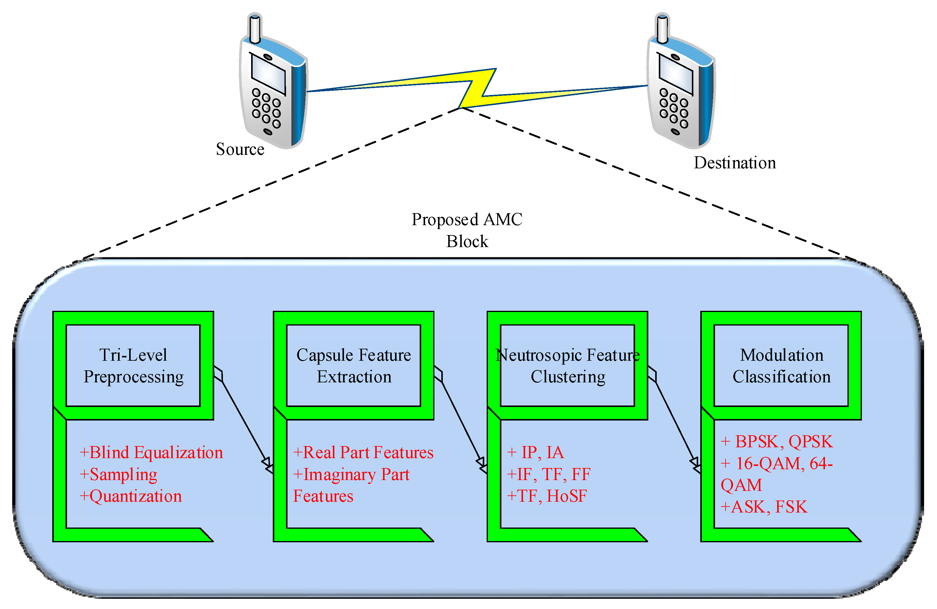
The aim of this study is to design a robust AMC method to provide improved results under low and high SNR rates. To achieve this goal, AMC2N formulates four sequential stages, namely, trilevel preprocessing, capsule-based feature extraction, feature clustering, and classification, as depicted in Figure 3.

In the first stage, three successive preprocessing steps, namely, blind equalization, sampling, and quantization, are applied. This stage is specifically designed to enhance the quality of the received signal. It executes the binary constant modulus algorithm (BCMA) to perform blind equalization, which evades the ISI of the signal. Sampling and quantization processes are performed to reduce the aliasing effects and bits required to represent the given signal.

In the second stage, the TL-CapsNet is used to improve feature extraction. To the best of our knowledge, no existing AMC utilizes a TL-CapsNet in FB-AMC. The TL-CapsNet algorithm is employed because it demonstrates satisfactory performance under low and high SNR rates. The preprocessed signal and estimated SNR value of the given signal are provided as input in the proposed TL-CapsNet. Seven essential features, namely, instantaneous amplitude, instantaneous phase, instantaneous frequency, time-domain features, frequency-domain features, transformation-domain features, and HOS features (cumulant and moment) are extracted. The features are extracted from the real and imaginary parts of the preprocessed signal to obtain enhanced results in the modulation recognition process. The TL-CapsNet uses two lanes to extract the features in parallel. Next, the extracted features are clustered based on feature similarity. The neutrosophic c-means (NCM) algorithm clusters the features from the real and imaginary parts of the signal. In general, the real part of a signal has a group of data, that is, the real-valued function, whereas the imaginary part contains zero. It can be determined by using complex Fourier transform [44] on the received signal. In terms of the real and imaginary parts, the signal can be represented as:

$$\mathbb{S}=\mathbb{R}+\mathbb{I}\mathbb{R}+(𝕚)I\mathbb{I}$$

(4)

where $\mathbb{R}$ represents the real part and $\mathbb{I}$ represents the imaginary part. In addition, $𝕚=-1$. Thus, implementing the MC process is easy, because NCM reduces the vast feature set of the signal. If a vast number of features are processed in the classifier, then, the performance of the classifier will degrade owing to the considerable amount of data processing. This work concentrates on six modulation schemes, specifically, QPSK, BPSK, ASK, FSK, 16-QAM, and 64-QAM. Subsequently, the performance of the proposed method is evaluated using six performance metrics, namely, feature extraction accuracy, classification accuracy, precision, recall, F-score, and computation time.

4.2. Trilevel Preprocessing

In FB-AMC scheme, preprocessing, plays a vital role because signal transmitted from the transmitter contains interference and noise, and thus degrades the performance of the FB-AMC system. Accordingly, the proposed AMC2N starts the process by improving the signal quality via trilevel preprocessing procedures, namely, blind equalization, sampling, and quantisation.

4.2.1. Blind Equalization

The main objective of blind equalization is to remove the ISI of the received signal, for example, in wireless communications systems, ISI occurs frequently because of limited bandwidth and multipath propagation [45]. The BCMA method is used to perform equalization in the AMC2N method. BCMA is chosen because it has been proven to perform better than the existing CMA method [46].

The BCMA method develops a new cost function and its iterative formula to eradicate the errors introduced by traditional CMA, such as excess and steady-state errors.

A received signal is expressed as [46]:

$$\mathfrak{x}\left(k\right)= \mathfrak{h}\left(k\right) ⨂ 𝓈\left(k\right)+n\left(k\right)$$

(5)

where $\mathfrak{h}\left(k\right)$ represents the channel impulse response, $𝓈\left(k\right)$ represents the transmitted data sequence, and $𝓈\left(k\right)$ represents the noise.

To remove ISI, an equalizer is imposed on the received signal. The output acquired from the proposed blind equalizer is approximated as follows:

$$𝕪\left(k\right)= {\displaystyle \sum }_{z=0}^{z_e - 1}{𝕨}^{*}\left(z\right)\mathfrak{x}\left(k-z\right)={𝕨}^h\mathfrak{x}\left(k\right)$$

(6)

where $\mathfrak{x}\left(k\right)=\left[\mathfrak{x}\left(k\right), \mathfrak{x}\left(k-1\right),\dots ,\mathfrak{x}\left(k-z_e+1\right)\right]$ signifies the input signal vector of the equalizer. The vector $𝕨={\left[w\left(0\right), w\left(1\right),..w\left(z_e-1\right)\right]}^T$ denotes the blind equalizer tap coefficient. The blind equalizer order is denoted as $z_e$. For each modulus value $M_v$, the respective attained samples are expressed as follows:

$$\phi =\left\{\mathfrak{x}\left(k\right)\Vert {𝕨}^h\mathfrak{x}\left(k\right)\left|- M_v\right|\le \zeta \right\}$$

(7)

where $\zeta$ signifies the discriminate threshold, and $\zeta =\min \left\{{\zeta }_n\right\}$ represents the partial discriminate value between $M_v$ and the residual modulus values.

The cost function generated using the BCMA method is represented as:

$$\underset{𝕨}{\min }{\left(\left|{𝕨}^h{\mathfrak{x}}_n\left(k\right)\right|-M_v\right)}^2$$

(8)

where ${\mathfrak{x}}_n\left(k\right)\in \phi$ and $M_v$ are the modulus values of the constellation points.

The proposed BCMA method updates the cost functions by using the following equation:

$${𝕨}_{i+1}={𝕨}_i-\delta \left(\left|{𝕨}_i^h{\mathfrak{x}}_n\left(i\right)\right|-M_v\right)\frac{{({𝕨}_i^h{\mathfrak{x}}_n\left(i\right))}^{*}}{\left|({𝕨}_i^h{\mathfrak{x}}_n\left(i\right)\right|}{\mathfrak{x}}_n\left(i\right)$$

(9)

where $\delta$ denotes the step size and the sample ${\mathfrak{x}}_n\left(i\right)$ represented in Equation (8) belongs to the upcoming set:

$${\phi }_i=\left\{\mathfrak{x}\left(k\right)\Vert {𝕨}_i^h\mathfrak{x}\left(k\right)\left|-M_v\right|\le \zeta \right\}$$

(10)

where ${\phi }_i$ signifies the group of utilized samples at the $i^{th}$ iteration process.

All of the above-mentioned processes and equations are utilized in the blind equalization process. The received signal is firstly processed with the blind equalization process by using a blind equalizer before the decision-making process is performed to remove the ISI from the received signal.

4.2.2. Sampling

Sampling is performed to reduce the aliasing effect of the given signal. The sampling signal provides the discrete time signal from the continuous time signal [47]. The notation $\mathbb{T}$ signifies the time interval amongst the samples, then, the moment at which the samples obtained are provided as $\mathfrak{N}\mathbb{T}$, where$\mathfrak{N}=-2, -1, 0, 1, 2$. Hence, the discrete time signal $x\left(\mathfrak{N}\right)$ related to the continuous time signal is denoted as [47]:

$$x\left(\mathfrak{N}\right)= x\left(\mathfrak{N}\mathbb{T}\right)$$

(11)

If a single sample occurs in each $\mathbb{T}$second, then, the sampling frequency ${\mathcal{F}}_s$ is defined as:

$${\mathcal{F}}_s=\frac{1}{\mathbb{T}}$$

(12)

The sampling frequency can also be defined in terms of the radians denoted by ${\varpi }_s$ as:

$${\varpi }_s=2\pi {\mathcal{F}}_s=2\pi /\mathbb{T}$$

(13)

From these processes, the sampling of the received signal is conducted, in which the discrete time signal is converted into a continuous signal. The values of the continuous function for every $\mathbb{T}$ second are also measured.

4.2.3. Quantization

Quantization is a significant process in modulation recognition [48]. It produces a received signal that has a range of discrete finite values. This study focuses on performing nonuniform quantization because it provides less quantization error as compared with the uniform quantization process [49]. We consider fixed signal $\overrightarrow{x}$ and utilize fixed positive integer $\varrho$. The Lloyd-Max quantizer [50] is adopted; it exploits two sets of parameters, as shown as follows:

• Bin boundaries $\overrightarrow{b}=\left(b_1, b_2,\dots , b_{n+1}\right)$ with min $\overrightarrow{x}=b_1<\dots b_n<b_{n+1}=1+\max \overrightarrow{x}$
• Replacement values $\overrightarrow{R_v}=\left(R_1, R_2,\dots , R_n\right)$

The quantization function changes $x$ values present in the bin (i.e., represented as ($b_j,b_{j+1}$)) with the value of $R_j$, which is expressed as [49]:

$$Q\left(x_i\right)=R_j; \mathrm{where} x_i\in \left[b_j,b_{j+1}\right]$$

(14)

The main goal of the Lloyd-Max quantizer is to reduce the quantization error, which is achieved via the following equation:

$$\mathcal{E}\left(\overrightarrow{b}, \overrightarrow{R}\right)={\displaystyle \sum }_{i=1}^m{\left|x_i-Q\left(x_i\right)\right|}^2$$

(15)

with these processes, the proposed Lloyd-Max quantizer algorithm quantizes the received signal, approximates the original signal, and separates the original signal from the added noise. It eases the further feature extraction and classification processes.

Figure 4 depicts the trilevel preprocessing steps. Briefly, blind equalization removes unwanted ISI from the signal. Next, sampling and quantization are performed to reduce aliasing and approximate the original signal. With the aid of these preprocessing procedures, the proposed AMC2N can improve the quality of received signals and enhance MC performance.

4.3. Two-Layer Capsule Network (TL-CapsNet)-Based AMC

Feature extraction and classification play a vital role in the MC of a given system. Most previous studies have concentrated on exploiting the CNN algorithm to extract features from a signal. Nonetheless, CNN loses the spatial information of a given signal during feature extraction, which leads to an inaccurate result in MC [51]. To solve this issue in conventional CNN, this study proposes a TL-CapsNet.

The TL-CapsNet is a recent deep learning algorithm that functions better than conventional CNN in feature extraction and classification [52]. We improve a TL-CapsNet by designing a novel TL-CapsNet architecture, as our work requires processing the real and imaginary parts of a signal. The proposed TL-CapsNet architecture is shown in Figure 5.

As shown in the figure, the input signal (modulated signal) is fed into our TL-CapsNet model. In the proposed model, the real and imaginary parts of the signal are processed in two separate lanes, that is, the real lane and imaginary lane. Consideration of the real and imaginary parts of the signal improves the robustness of the work in low SNR scenarios. Each lane consists of a convolutional (Conv) layer, a convolutional capsule layer (with PrimaryCaps), and a hidden caps layer (DigitCaps). The proposed TL-CapsNet performs the following major processes:

• Feature extraction;
• Feature clustering;
• Classification.

4.3.1. Feature Extraction

Unlike conventional CNN, the TL-CapsNet considers spatial information during feature extraction, which can lead to an improvement in feature extraction accuracy during AMC. The dynamic routing process of the TL-CapsNet assists in feature extraction. In general, dynamic routing is performed in the DigitCaps layer. As shown in Figure 5, the real and imaginary parts and SNR of the signal are fed into the convolution layer of the TL-CapsNet. Next, a conventional integer encoding method is used for encoding. Encoding is the process of converting each input signal into codes. Each input signal is mapped into integer values. Next, the features in the signal are extracted in the primary caps, which match the ultimate caps in the DigitCaps layer. Ultimate high-level features can be extracted from the signal (real and imaginary parts) by processing the signal in the primary caps and DigitCaps. From the DigitCaps, we extract the features used in the NCM clustering. Figure 3 illustrates the proposed TL-CapsNet for feature extraction. To the best of our knowledge, this study is the first to exploit a TL-CapsNet in FB-AMC. The proposed TL-CapsNet performs better than existing CNNs by producing an effective feature extraction process, which does not lose any spatial-related information of the signal [53]. The convolutional layer comprises 256 × 9 convolutional kernels and a rectified linear unit (ReLU) activation function with stride 1. It primarily performs a convolutional operation to extract low-level features from the real and imaginary parts of a signal. After the low-level features are extracted, the output of the convolutional network is fed into two layers, namely, the primary cap and digit cap. The primary capsule refers to multidimensional entities at the lowest level and comprises the convolutional capsule layer incorporating 32 8D capsule channels individually for each primary capsule. The digit cap layer comprises 16D capsules for every digit class with 10 vectors.

It also requires less training time and data requirements to train the network. Furthermore, the TL-CapsNet can work under a new or unseen variation of a given input class without being trained with the data. This capability is essential in the proposed MC, because the received signal has large SNR rate variations (i.e., changes between low and high SNR rates). Thus, the proposed AMC2N can extract features under different SNR variations. The SNR is computed by considering the signal power ($P_S$) and noise power ($P_N$) extracted from the received signal as ($SNR=P_S/P_N$). For the SNR calculation, this work uses a conventional method, namely, split-symbol moment estimation, which is discussed in [54]. The SNR is estimated through the following formulation:

$$SNR=\frac{U^{+}-U^{-}}{U^{-}}$$

(16)

where $U^{+}$ is the average total power and $U^{-}$ is the average power of the signal, which can be represented as:

$$U^{\pm }=\frac{1}{N}{\displaystyle \sum }_{j=1}^N{\left|u_j^{\pm }\right|}^2$$

(17)

The SNR is estimated for $N$ number of samples and $j\in N$. To extract features, the proposed TL-CapsNet considers input such as the preprocessed signal and estimated SNR of the given signal. SNR information is given as input to the TL-CapsNet to extract features under different SNR variations and increase the robustness of the proposed AMC2N to work within large SNR variations.

The TL-CapsNet considers the real (${\mathfrak{r}}_p$) and imaginary (${\mathfrak{T}}_p$) parts of the preprocessed signal. The real and imaginary parts of the signal are considered, because modulated signals change in phase and amplitude information with respect to the shape of the constellation diagram. This variation affects the imaginary and real parts of a complex signal. Thus, the proposed technique can work properly in such varied conditions by considering both parts. In the TL-CapNet, the dynamic routing procedure assists in the feature extraction. Feature extraction is performed by the PrimaryCaps. Furthermore, the features are matched in the hidden caps layer through the dynamic routing process. The dynamic routing process assists in providing the output of the primary capsules to the hidden capsules. The routing agreement works on the ability of the hidden capsules to predict the parent’s output.

Dynamic routing is performed between the two successive capsule layers (i.e., the primary cap and digit cap). It is exploited to resolve the issue in which a high-rate capsule transfers the output value of a low-rate capsule. All routing logits denoted as ${𝓀}_{\mathcal{U},\mathcal{V}}$ are initialised as 0. The routing logits are updated by increasing the iteration level. The formula for updating the routing logits is given in [51] as:

$${𝓀}_{\mathcal{U},\mathcal{V}}={𝓀}_{\mathcal{U},\mathcal{V}}+{\widehat{𝓊}}_{\mathcal{V}|\mathcal{U}}.{\mathfrak{V}}_{\mathcal{V}}$$

(18)

where:

$${\widehat{𝓊}}_{\mathcal{V}|\mathcal{U}}={𝓊}_{\mathcal{V}|\mathcal{U}} \times {\mathcal{W}}_{\mathcal{U}\mathcal{V}}$$

(19)

where ${\widehat{𝓊}}_{\mathcal{V}|\mathcal{U}}$ represents the predicted vectors from the capsule layer $\mathcal{U}$ in the network, ${𝓊}_{\mathcal{U}}$ represents the output from the capsule layer, and ${\mathcal{W}}_{\mathcal{U}\mathcal{V}}$ represents the weighted matrix.

The total input in the first layer of the capsule is expressed as:

$${\mathcal{S}}_{\mathcal{U}}={\mathcal{C}}_{\mathcal{U}\mathcal{V}} \times {\widehat{𝓊}}_{\mathcal{V}|\mathcal{U}}$$

(20)

where ${\mathcal{C}}_{\mathcal{U}\mathcal{V}}$ signifies the coupling coefficient obtained during the iterative process using the following equation:

$${\mathcal{C}}_{\mathcal{U}\mathcal{V}}=\frac{e^{{\mathcal{C}}_{\mathcal{U}\mathcal{V}}}}{{{\displaystyle \sum }}_{i=1}^n{e}^{{\mathcal{C}}_{\mathcal{U}i}}}$$

(21)

The pseudocode for the proposed TL-CapsNet-based feature extraction is given as follows:

Pseudocode 1 depicts the processes involved in the capsule-based feature extraction and initializes the input and output nodes of the network. The aforementioned processes are used to extract features from the real and imaginary parts of the signal. Seven features, namely, instantaneous amplitude, instantaneous frequency, instantaneous phase, time-domain features, frequency-domain features, transformation-domain features, and HOS features are extracted from the received signal using the TL-CapsNet. HOS features play a vital role in MC, because they are robust under different SNR rates, thereby, increasing the efficacy of the proposed capsule-based feature extraction. Likewise, the extracted instantaneous features are highly significant in MC, because they provide the accurate condition of the received signal. On the basis of five primary features, this study further introduces 15 subfeatures. These features are considered to attain enhanced results in the classification process. Features are important to attain high accuracy during the classification process. The considered features are indicated in

Table 2. Feature description.

Features	Subfeatures	Formula [24]
Instantaneous Features	Amplitude	$X\left(t\right)=a\left(t\right)cos\left({\omega }_{0}t\right)$
	Phase	$X\left(t\right)=a\left(t\right)\cos \left(\varnothing t\right)$
	Frequency	$F\left(t\right)=\frac{d}{dt}\varnothing t$
Time-domain Features	Variance	$F_{var}=\left[X\left(t\right)-F_m\right]$
	Standard deviation	$F_{std}=\sqrt{\frac{{{\displaystyle \sum }}_{i=1}^n{\left(X\left(t\right)-F_m\right)}^2}{n-1}}$
	Skewness	$F_{skew}=\frac{{{\displaystyle \sum }}_{i=1}^n{\left(X\left(t\right)-F_m\right)}^3}{\left(n-1\right)F_R^3}$
	Kurtosis	$F_{kur}=\frac{{{\displaystyle \sum }}_{i=1}^n{\left(X\left(t\right)-F_m\right)}^4}{\left(n-1\right)F_R^4}$
Frequency-domain Features	Mean frequency	$F_m=\frac{{{\displaystyle \sum }}_{i=1}^{ n}(X\left(t\right)}{n}$
	Median frequency	$F_{me}=\frac{{{\displaystyle \sum }}_{i=1}^{ n}X\left(t\right)}{2}$
	Power bandwidth	$F_p=\frac{{{\displaystyle \sum }}_{i=1}^{ n}(pX\left(t\right)}{n}$
	Zero cross rate	$F_z={\displaystyle {\displaystyle \sum }_{i=1}^{ n}}sgn X\left(t\right).x\left(t+1\right)$
Transformation Features	Mean absolute value	$F_{ma}=\frac{1}{n}{\displaystyle {\displaystyle \sum }_{i=1}^n}\left|X\left(t\right)\right|$
	Root mean square	$F_R=\frac{{{\displaystyle \sum }}_{i=1}^{ n}(X{\left(t\right)}^2}{n}$
HOS Features	Cumulant	$F_{cu}=logE\left[e^{X\left(t\right)}\right]$
	Moment	$F_{mo}={\displaystyle {\displaystyle \sum }_{i=1}^n}\frac{X\left(t\right)}{t}$

Note: $X\left(t\right)$ is represented as signal series, where t = 1, 2, …, n.

.

Pseudocode 1. Dynamic routing-based feature extraction in TL-CapsNet.

Require:${\mathfrak{r}}_p,{\mathfrak{T}}_p$, SNR Ensure: Extracted Features

Initialize$\to$ nodes (input and output); Add$\to$ Edges of nodes using broadcasting; Design two-lanes Divide $Signal$ into ${\mathfrak{r}}_p , {\mathfrak{T}}_p,$ Compute SNR For each lane //Routing------------ For all capsule $\mathcal{U}$ in layer$𝓁$ and capsule $\mathcal{V}$ in layer ($𝓁+1$): ${𝓀}_{\mathcal{U},\mathcal{V}}\leftarrow 0;$ For (each iteration $\mathcal{I}$) do    Compute$\to$softmax function for all capsule $\mathcal{U}$ in layer $𝓁$; Compute$\to$softmax function for all capsule $\mathcal{V}$ in layer $𝓁+1$;    Update$\to$weight ${𝓀}_{\mathcal{U},\mathcal{V}}$ using Equation (15);  End for Emit (${\mathfrak{V}}_{\mathcal{V}}$);

4.3.2. Feature Clustering

Once the features are extracted in the primary caps and mapped in the DigitCaps, the features are clustered by computing similarity in the concatenate layer. In this stage, the NCM clustering process is proposed to restructure and reorganize the extracted features to improve the accuracy of the proposed AMC. If raw extracted features are directly given to the classification, then, the SoftMax layer must process the raw features on its own. Its performance could degrade if the features are affected by noises. Thus, clustering the features can help in grouping them into predetermined groups. In addition, this process can group noises into one specific group. By providing substantial systematically processed features, classification is believed to improve the classification of modulation schemes. As previously mentioned, a limited number of works have focused on reducing the difficulty faced by the classification module during modulation detection. In the present work, the AMC2N concentrates on reducing AMC difficulties via the feature clustering process. The clustering of feature vectors from real and imaginary parts is achieved by implementing the NCM algorithm. The proposed NCM clustering method is chosen, because it has been proven to demonstrate better performance than the fuzzy c-means clustering algorithm in terms of avoiding inaccurate results [24].

Pseudocode 2 describes the procedures involved in the feature clustering process using the NCM algorithm. It requires three membership functions, namely, the truth set${\mathbb{T}}_i$, indeterminate set${\mathbb{I}}_i$, and false set${\mathbb{F}}_i$. It initially estimates the cluster center by using the following equation [24]:

$$C_c=\frac{{{\displaystyle \sum }}_{i=1}^n{({\sigma }_1{\mathbb{T}}_i)}^m.f_i}{{{\displaystyle \sum }}_{i=1}^n{({\sigma }_1{\mathbb{T}}_i)}^m}$$

(22)

where ${\sigma }_1$ represents the weight vector and $m$ denotes the constant value.

Pseudocode 2. Feature clustering in TL-CapsNet.

Require:$\mathbb{T}, \mathbb{I},\mathbb{F},{\sigma }_1,{\sigma }_2,{\sigma }_3$ Ensure: Clustered features

Initialize$\to \mathbb{T}, \mathbb{I},\mathbb{F},{\sigma }_1,{\sigma }_2,{\sigma }_3$;  For (each feature $f_i\in f_n)$ do    Estimate$\to$Cluster center ($C_c$) vector using Equation (22);    Estimate$\to C_{ci}$ using Equation (23);    Update$\to {\mathbb{T}}_i$, ${\mathbb{I}}_i$, ${\mathbb{F}}_i$ using Equations (25)–(27) respectively;    $T{M}_i=[{\mathbb{T}}_i$, ${\mathbb{I}}_i$, ${\mathbb{F}}_i]$;    If $(T{M}_i>TM)$       Assign$\to f_i\to C^{th} cluster$;      End If    If ($\left|{\mathbb{T}}_{i+1}-{\mathbb{T}}_i\right|<\partial )$       Stop$\to$Clustering Process;     Else       Continue$\to C_c$ estimation;     End If  End for

The proposed NCM algorithm formulates the objective function to form clusters. The function is given as:

$$\left(\mathbb{T}, \mathbb{I},\mathbb{F},C\right)= {\displaystyle \sum }_{i=1}^n{\displaystyle \sum }_{j=1}^C{({\sigma }_1{\mathbb{T}}_{ij})}^m.\Vert f_i-C_j\Vert {}^2+{({\sigma }_2{\mathbb{I}}_{ij})}^m.\Vert f_i-{\widehat{C}}_{ci}\Vert {}^2+{\alpha }^2{({\sigma }_3{\mathbb{F}}_i)}^m.\Vert f_i-{\widehat{C}}_{ci}\Vert {}^2$$

(23)

where ${\widehat{C}}_{ci}$ is estimated with respect to the indices of the first and second largest values of ${\mathbb{T}}_{ij}$ obtained via comparison using the following equation:

$${\widehat{C}}_{ci}= \frac{C_{gi}+C_{hi}}{2}$$

(24)

where $C_{gi}$ and $C_{hi}$ are cluster members.

The first part of Equation (23) signifies the degree with respect to the main clusters, whilst the second part of the equation represents the degree with respect to the cluster boundary. The third part of the equation denotes the outlier or noise of the clusters.

The three membership functions are then updated using the following expressions:

$${\mathbb{T}}_{ij}=\frac{𝓀}{{\sigma }_1}{\left(f_i-C_c\right)}^{\frac{2}{m-1}}$$

(25)

$${\mathbb{I}}_i= \frac{𝓀}{{\sigma }_2}{\left(f_i-{\widehat{C}}_{ci}\right)}^{\frac{2}{m-1}}$$

(26)

$${\mathbb{F}}_i= \frac{𝓀}{{\sigma }_3}{\left(\alpha \right)}^{\frac{2}{m-1}}$$

(27)

$$𝓀= {\left(\frac{\rho }{m}\right)}^{\frac{1}{m-1}}$$

(28)

where $\rho$ signifies the constant parameter in the NCM clustering process.

With the aid of these processes, the proposed NCM algorithm clusters the features from the real and imaginary parts. It initially estimates the cluster center, and then formulates the objective function to cluster the features extracted from the real and imaginary parts of the signal. This study reduces the considerable feature set processing during classification through clustering.

In Figure 6, NCM cluster-based feature clustering is depicted. The features extracted from each signal are clearly clustered into seven clusters. In the testing phase, comparing the features with the cluster centers instead of comparing each feature is possible.

4.3.3. Modulation Classification at Softmax Layer

After the feature clustering process in the concatenate layer, the signal is classified in the SoftMax layer. The output vector of the capsule is constructed using the squash function, which is expressed as:

$${\mathfrak{V}}_{\mathcal{V}}=\frac{\Vert {\mathcal{S}}_{\mathcal{U}}\Vert {}^2\Vert {\mathcal{S}}_{\mathcal{U}}\Vert }{1+ \Vert {\mathcal{S}}_{\mathcal{U}}\Vert {}^2\Vert {\mathcal{S}}_{\mathcal{U}}\Vert }$$

(29)

where ${\mathfrak{V}}_{\mathcal{V}}$ represents the vector output of the capsule layer $\mathcal{U}$. It is expressed in a probability manner; thus, it is adjustable between the values [0, 1]. Based on the squash function, the SoftMax layer determines the output-proposed modulation. The output is delivered by the fully connected dense layer with 128 units. For each class, margin loss is computed. For class $k$, the margin loss is given as:

$$M{L}_k=T_{k}max{\left(0,m^{+}-v_k\right)}^2+\lambda \left(1-T_k\right)max{\left(0,v_k-m^{-}\right)}^2$$

(30)

where $T_k$ is 1 if a sample is presented for class $k$ and 0 otherwise. All other variables are the upper and lower bounds set in the range of [0, 1]. In this work, we consider $m^{+}$ as 0.9 and $m^{-}$ as 0.1. In the decoder unit, the features are reconstructed, and reconstruction loss is computed as follows:

$$RL=MSELoss\left(X,X^{\prime }\right)$$

(31)

Reconstruction loss is computed in terms of the mean squared error between the original signal $X$ and reconstructed signal $X^{\prime }$. In our proposed TL-CapsNet, the current extracted features are compared with the cluster centroid, which is computed in the concatenate layer to produce the final classification output. Involvement of the feature clustering process in the TL-CapsNet minimizes classification time by reducing comparisons made among features. In Figure 7, we provide the detailed pipeline architecture of the proposed work. When two nodes communicate with each other, the proposed AMC block is executed at the destination to identify the modulation scheme accurately.

In summary, the proposed AMC2N technique firstly performs trilevel preprocessing, namely, blind equalization, sampling, and quantization. ISI, aliasing, and noise in the received signal are removed to ease the proceeding processes. The proposed AMC2N technique extracts features from the real and imaginary parts of the signal using a TL-CapsNet, thereby, making the proposed AMC2N the first AMC technique to utilize a TL-CapsNet in three aspects. Firstly, features are extracted in parallel through two lanes for the real and imaginary parts. Secondly, the extracted features are clustered in the concatenate layer to boost the classification process. Lastly, the SoftMax layer classifies the benefits of the algorithms included in the proposed AMC2N, which are summarized in

Table 3. Benefits of the proposed algorithm in automatic modulation classification using a feature clustering-based two-lane capsule network (AMC2N).

Algorithms	Benefits
BCMA	This algorithm is used to reduce the ISI of the received signal. It enhances the quality of the signal and exhibits improvement under heavy-noise conditions. These benefits can improve the performance of the feature extractor and classifier.
TL-CapsNet	This algorithm is used to improve feature extraction accuracy. It provides enhanced performance under low and high SNR rate variations. It also requires minimal data during training and consumes minimal processing time. It considers the real and imaginary parts of a signal to enhance feature extraction performance. Moreover, it considers the SNR of a given signal as input to provide robust performance under SNR variations. Accuracy of the modulation classification is improved through feature clustering and modified loss function. Feature clustering also minimizes the time for classification.

.

5. Result and Discussion

This section is dedicated to a description of the investigation of the performance of the proposed AMC2N method by using the simulation results. To characterize the efficacy of the proposed AMC2N method, this section is further divided into three subtopics, namely, experimental setup, result analysis, and research summary.

5.1. Experimental Setup

In this subsection, the simulation scenario of the proposed AMC2N method is discussed. For evaluation purposes, this study generates simulated training and test signals with 1024 samples for MC by using the parameters presented in

Table 4. Modulation.

Parameter	Value
Carrier frequency	30 MHz
Sampling rate	1.25 MHz
Symbol rate	300 kHz
Number of symbol	1024

. Signals with six modulation schemes, namely, QPSK, BPSK, ASK, FSK, 16-QAM, and 64-QAM are generated. In

Table 5. Two-layer CapsNet (TL-CapsNet) algorithm parameters setting.

Parameter	Value
Number of capsules	32
Activation function	ReLU
Number of fully connected layers	3

, the value of all parameters proposed method are included.

The generated signals are incorporated with AWGN for SNR rates between −10 and 10 dB. The objective of incorporating AWGN is to evaluate the capability of the proposed AMC2N to work under a noisy environment.

To validate the performance of the proposed AMC2N approach, five performance metrics, namely, accuracy, precision, recall, F-score, and computation time, are considered.

Accuracy ($\mathcal{A}$) is the most instinctual metric to measure the system performance. It is measured by computing the ratio of the correctly estimated modulation scheme to the original modulation scheme of the received signal. It can be approximated as follows:

$$\mathcal{A}=\frac{{\mathcal{T}}_1+{\mathcal{T}}_2}{{\mathcal{T}}_1+{\mathcal{T}}_2+{\mathcal{F}}_1+{\mathcal{F}}_2}$$

(32)

where ${\mathcal{T}}_1$ represents the true positive, ${\mathcal{T}}_2$ represents the true negative, ${\mathcal{F}}_1$ represents the false positive, and ${\mathcal{F}}_2$ represents the false negative. As the work is about multi-class classification, we construct confusion matrix by considering actual class and predicted class for all classes. Then, we compute the metrics from the confusion matrix.

Precision ($\mathcal{P}$) is one of the crucial metrics to measure the exactness of the AMC2N approach. It is measured by estimating the ratio of the relevant MC result to the total obtained modulation result. It is expressed as follows:

$$\mathcal{P}=\frac{{\mathcal{T}}_2}{{\mathcal{T}}_1+{\mathcal{F}}_1}$$

(33)

Recall ($\mathcal{R}$) is a significant metric to measure the completeness of the proposed AMC2N approach. It is estimated by calculating the total amount of the relevant MC results that are actually retrieved. It is expressed in mathematical form as follows:

$$\mathcal{R}= \frac{{\mathcal{T}}_1}{{\mathcal{T}}_1+{\mathcal{F}}_2}$$

(34)

F-score ($F_S$) validation is used to measure the accuracy of the test results. It is defined as the joint evaluation of the precision and recall parameters. It is expressed as follows:

$$F_S=\frac{2\ast \mathcal{P}\ast \mathcal{R}}{\mathcal{P}+\mathcal{R}}$$

(35)

Computation time is essential to validate the efficacy of the proposed AMC2N approach in terms of providing computational processing time that is as low as possible. It is measured by considering time elapsed to complete the MC process.

5.2. Result Analysis

The simulation results of the proposed AMC2N are compared with those of existing methods, in particular, CNN [38], R-CNN [39], CL [40], and LBP [41]. The reason behind selecting these methods for comparison is that the contributions of these methods are similar to the contributions, i.e., preprocessing, feature extraction, and classification of the proposed method.

Table 6. Comparison of extraction methods.

.	Core Intention	Modulation Schemes Considered for Evaluation	Performance under SNR Variations		Downsides
			Low SNR	High SNR
CNN [38]	To provide an end-to-end process in FB-AMC	2-PSK, 4-PSK, 16-QAM, 16-APSK, 32-APSK, 64-QAM	×	√	Unrobust to SNR variations Loss of spatial information of the signal
R-CNN [39]	To create MC robust to SNR variations	ASK, FSK, PSK, QAM	×	√	High difficulty during MC Lack of significant features, including instantaneous and time features
CL [40]	To introduce CL into FB-AMC	ASK, FSK, PSK, QAM	×	√	Considerable training time Lack of essential preprocessing steps
LBP [41]	To implement LBP-based feature extraction and ML-based classification in AMC	BPSK, QPSK, 8-PSK, QAM	×	√	Unoptimal features extracted due to high false positive result Slow classification process

describes the comparison of the existing methods with their core intention, modulation scheme considered, performance under SNR variations, and downsides. The notations of × and √ signify the poor and moderate performance, respectively, of the existing methods under SNR variations.

All parameters are tested under two scenarios, as follows:

Scenario 1 (with varying SNR rates): In this scenario, the SNR range is varied, and the number of samples is fixed. This scenario is considered to prove the efficacy of our proposed work in varying SNR ranges, that is, low and high SNR scenarios from −10 dB to 10 dB with an increasing step of 2 dB.

Scenario 2 (with varying sample numbers): In this scenario, the SNR value is fixed, and the number of samples is varied. In this scenario, the efficacy of the proposed TL-CapsNet is tested using low and high numbers of samples from 25 to 200 with an increasing step of 25.

5.2.1. Effect of Accuracy

Accuracy is examined in both scenarios to evaluate the efficacy of our proposed work. Feature extraction and classification accuracy is determined in both scenarios. The accuracy of the proposed method is compared with that of existing methods, such as CNN, R-CNN, CL, and LBP. Figure 8 and Figure 9 present the results of the percentage accuracy of the feature extraction process for Scenarios 1 and 2.

As presented in Figure 8, the proposed AMC2N approach demonstrates better performance than the existing methods in Scenario 1. The results show that the proposed TL-CapsNet demonstrates a high performance of more than 95% under low and high SNR rates. The introduction of the real and imaginary parts of a given signal assists the proposed AMC2N to extract accurate features, which enhances the feature extraction performance. In general, in prior works, feature extraction is performed by neglecting the imaginary parts of a signal, which is the reason behind low accuracy. In addition, we compute the SNR as a feature and include it in the feature extraction process to improve accuracy. As a result, performance is enhanced from 80% to 90% for −10 dB to −2 dB values and up to more than 90% subsequently. The analysis shows that accuracy increases as the SNR range increases. Similarly, when the SNR is reduced to lower than −10 dB, accuracy will degrade. However, variation in the accuracy range is 16% for SNR variations. Thus, the proposed AMC2N can maintain accuracy better than the existing methods even in low SNR ranges. Moreover, the feature extraction performance of the other methods is poor. This result can be attributed to their inefficiency in extracting features under low SNR rates (i.e., feature extraction accuracy is less than 50% for an SNR from −10 dB to −2 dB). On the basis of the results, the proposed method can successfully increase accuracy to a maximum of 58% under low SNR rates and to 20% in high SNR rates as compared with the other methods.

In Figure 9, the accuracy of the proposed and existing methods is compared in Scenario 2, that is, based on varying sample sizes. The sample size denotes the number of samples considered for classification. The proposed method achieves better accuracy than the existing methods. This result also supports the advantage of the proposed work processes for the real and imaginary parts of the signal. Moreover, the proposed model can learn more features than the existing methods. Thus, the proposed method achieves improved accuracy up to 70% even with small sample sizes. Furthermore, the proposed work can achieve feature extraction accuracy of over 45%, which is greater than that of the existing CNN, R-CNN, CL, and LBP models at 25 samples.

In Figure 10, classification accuracy is compared in Scenario 1, and as expected, the proposed AMC2N is the best AMC method. It can successfully demonstrate accuracy of more than 95% for all SNR rates. This result is observed, because feature extraction is a significant classification process. Moreover, the proposed work attains superior accuracy in feature extraction in both scenarios, which indicates that classification accuracy is likewise improved. Feature clustering reduces classification complexity and helps improve the performance of the proposed AMC2N. CNN, R-CNN, and CL demonstrate a classification accuracy of only more than 75% for 8 dB and 10 dB SNR rates. The LBP method produces the worst classification rate, in which classification accuracy for 8 dB and 10 dB tested SNR rates is less than 72%. The existing methods demonstrate poor classification accuracy as compared with the proposed AMC2N approach, especially under low SNR rates (i.e., accuracy of less than 50% from −10 dB to −2 dB SNR rates). These methods use raw extracted features, which are large in number. This condition leads to an increment in the model complexity of the existing methods, which affects their classification accuracy. The main issue to note is that the proposed AMC2N method achieves accuracy of up to 95%. The analysis shows that the proposed work achieves the objective of accurate classification in low SNR scenarios. This result is obtained, because the proposed AMC2N initially augments the received signal through optimum preprocessing steps. Next, the noiseless signal is obtained and further processed for classification. In the classification, the proposed TL-CapsNet classifier considers the SNR range of the current signal as input. In addition, the separation of the real and imaginary parts of the signal for feature extraction improves accuracy. In general, the proposed AMC2N method successfully increases the accuracy percentage by up to 59% under low SNR rates and up to 18% under high SNR rates as compared with the existing methods.

In Figure 11, classification accuracy is verified based on varying sample sizes. When the sample size is small, the existing methods (i.e., CNN, R-CNN, and so on) demonstrate accuracy, as they require enormous amounts of samples for effective classification. In real time, a signal is affected by noises, which are not processed in prior works. However, the proposed work demonstrates accuracy higher than 65%, even with 25 samples, owing to the involvement of optimum feature learning and feature clustering processes.

In Figure 12, the accuracy confusion matrix for the proposed AMC2N is presented. Most of the different types of modulation signals are classified correctly, which is above 90%. This result shows that the proposed AMC2N demonstrates high capability in classifying different types of modulation signals.

5.2.2. Effect of Precision

Precision is measured in both scenarios to evaluate the efficacy of our proposed work. The precision performance of the proposed AMC2N method is compared with that of the existing methods. Figure 13 and Figure 14 present the results of the precision percentage.

Figure 13 and Figure 14 show that the performance of the proposed AMC2N method is better than that of the existing methods in both scenarios. This superiority is achieved via our proposed mechanisms before the MC process. Our work initially improves the quality of the received signal through trilevel preprocessing. Three preprocessing steps, namely, blind equalization, sampling, and quantization, are performed to enhance the quality of the received signal. The three processes remove ISI, aliasing, and noise from the signal. If these deficiencies are removed from the received signal, then, signal quality is improved. This process of enhancing received signal quality provides improved feature extraction and classification results. Thus, performance is enhanced under the proposed work even for signals with low SNR rates. Moreover, we achieve improved results with small sample amounts.

The existing methods perform poorly as compared with our proposed work. In addition, they lack effective preprocessing steps, such as blind equalization, sampling, and quantization. Thus, the precision measure is affected during the evaluation process. CNN, R-CNN, and CL achieve high precision of more than 80%, and LBP has a precision rate of less than 80% at an SNR of 10 dB. These state-of-the-art methods achieve less than 30% at −10 dB and less than 85% at 10 dB. By contrast, our proposed method increases accuracy by up to a maximum of 58% at −10 dB and a minimum of 20% at 10 dB as compared with the existing methods. Furthermore, our proposed work achieves accuracy higher than 65% with 25 samples.

5.2.3. Effect of Recall

The recall validation metric is measured by varying the sample size and SNR range to prove the efficacy of the proposed work. The recall metric of the proposed method is compared with that of the existing methods.

Figure 15 and Figure 16 show that the recall performance of the proposed method is better than that of the other methods, with varying SNR ranges and sample sizes. Substantial features are required to achieve an improved recall result in AMC. Hence, our proposed AMC2N method extracts features from real and imaginary parts of the signal. Six different features, namely, instantaneous features (amplitude, frequency and phase), time-domain features, frequency-domain features, transformation-domain features, and HOS features are extracted. These features play a vital role in the classification of modulation schemes. Among them, HOS features are robust to SNR variations, and thus can enhance classification performance.

The existing methods provide poor results in recall performance as compared with the proposed work owing to their inefficiency in extracting effective features in the feature extraction process. CNN, R-CNN, CL, and LBP achieve recall lower than 30% when the sample size is small and 50% under low SNR rates. In the worst scenario, the proposed work demonstrates better performance than the existing works.

5.2.4. Effect of F-Score

The F-score measure is evaluated in the two scenarios. The F-score metric of the proposed method is compared with that of the existing methods.

Figure 17 and Figure 18 show that the performance of the proposed work, in terms of the F-score measure, is better than that of the existing methods. This superiority is attributed to our proposed similar feature clustering-based modulation scheme classification process. Clustering extracted features reduces the difficulty of the ML-based classifier. We provide input as the center value of each cluster feature, and thus avoid substantial feature processing in the ML-based classifier. Hence, our work enhances F-score performance during MC.

The existing methods demonstrate poor F-score performance as compared with the proposed work owing to their poor performance in handling the substantial number of features extracted from the given signal. They achieve less than 83% at an SNR of −10 dB and more than 95% at an SNR of 10 dB. Moreover, they achieve more than 60% with low sample amounts and 96% with high sample amounts. The proposed method increases F-score performance by up to a maximum of 26% at 10 dB and a minimum of 58% at −10 dB as compared with the existing methods.

5.2.5. Effect of Computation Time

Computation time is measured by increasing the sample size considered in the classification. The computation time of the proposed method is compared with that of the existing methods.

As shown in Figure 19, the proposed method requires less computation time than the existing methods. Our proposed TL-CapsNet performs fast and reduces training time. Furthermore, involvement of the feature clustering process reduces the time needed to classify the modulation scheme of the given signal. Our proposed model processes only cluster center feature values, and thus requires less time as compared with vast feature processing. Hence, our method reduces computation time as compared with the existing methods.

The existing methods require considerable computation time to implement the FB-AMC. They require 112 ms for 25 samples and 312 ms for 200 samples. Specifically, CL and LBP need more than 500 ms for 200 samples. By contrast, our proposed method reduces computation time to a maximum of 255 ms for 200 samples and a minimum of 72 ms for 25 samples as compared with the existing methods.

5.2.6. Impact of TL-CapsNet in Results

This research introduces a new capsule-based feature extraction procedure to boost AMC accuracy. The results show that the proposed method achieves improved accuracy and performs well even in low SNR scenarios. In this section, we compare the results of our proposed work with those of the existing methods.

In the absence of a TL-CapsNet, that is, with CapsNet, accuracy is low, specifically, lower than 75%. By incorporating a TL-CapsNet, accuracy can be improved by up to 96%. In

Table 7. Numerical result of proposed.

Method	Accuracy (%)		Precision (%)	Recall (%)	F-Score (%)	Computation Time (ms)
	FE	C
ACM2N with CapsNet	73	75	70	72	70	63
AMC2N without feature clustering	88	87.5	75	77	74	62
Proposed AMC2N	97	96.5	85	89	85	50

, we compare the proposed work with the base algorithms. At the same time, the absence of NCM clustering directly affects feature extraction accuracy by up to 88%. This accuracy level is achieved with the help of a TL-CapsNet with reconstruction mechanisms. Classification accuracy is also affected, as it relies on extracted features. In addition, the feature clustering process directly affects computation time, that is, the proposed method with a feature clustering process reduces computation time by up to 50 ms, which is 12 ms less than that of the base algorithms. Overall, the proposed work achieves improved performance in terms of accuracy and time consumption.

5.2.7. Complexity Analysis

In this subsection, we analyse the complexity of the proposed AMC approach and compare the complexity with the existing works. The comparison is summarized in

Table 8. Complexity analysis.

Method	Complexity
Proposed AMC2N	$O\left(\mathrm{N}+3\right)N$
ML	$O\left(N^n\right)+1$
RCNN	$O\left(N^2\right)+O\left(N\right)$
CNN	$O\left(3N+N^2\right)$
LBP	$O\left(2N+N^2\right)$

.

The analysis summarizes the complexity of proposed and existing works. It can be seen that the complexity of proposed approach is lower than the existing works. The complexity of the proposed work includes computations needed by preprocessing ($N+3$) and classification $(N$). Thus, the proposed approach achieves promising outcomes with lower complexity.

6. Conclusions

The contributions of AMC to digital wireless communication systems have increased dramatically. This study aims to achieve improved MC accuracy under low and high SNR rates. In this regard, a robust AMC method, namely, the AMC2N, is proposed. The AMC2N executes four significant processes to achieve enhanced performance. Moreover, preprocessing is executed to enhance the quality of the received signal by applying three sequential processes, namely, blind equalization, sampling, and quantization. We design a novel TL-CapsNet that performs feature extraction, feature clustering, and classification. Seven sets of significant features are extracted from the imaginary and real parts of the signal, which are clustered to boost the classification. Finally, classification is performed in the SoftMax layer with a modified loss function. It considers six modulation schemes for classification, specifically, QPSK, BPSK, ASK, FSK, 16-QAM, and 64-QAM. The experiment results show that the proposed AMC method demonstrates superior performance. The fusion of four important phases in the proposed work supports the improved efficiency. The acquired results are compared with those of existing methods (i.e., CNN, R-CNN, CL, and LBP) in terms of accuracy, precision, recall, F-score, and computation time. The results prove that the proposed AMC2N method outperforms the existing methods in all the metrics.