Abstract
The SOGI-FLL (second-order generalized-integrator frequency-locked-loop) is a well-known and simple adaptive filter that allows estimation of the parameters of the grid voltage with a small computational burden. However, this structure has shown to be sensitive to the events of voltage sags and swell faults, especially to voltage sags that deeply distort the estimated frequency. In this paper an algorithm is proposed to face the fault that modifies the SOGI-FLLs gains in order to achieve a better transient response with a reduced perturbation in the estimated frequency. The algorithm uses the SOGI’s instantaneous and absolute error to detect the fault and change the SOGI-FLL gains during the fault. Moreover, the average of the absolute error is used for returning to normal operating conditions. The average value is obtained by means of a single low pass filter (LPF). The approach is easy to implement and represents a low computational burden for being implemented into a digital processor. The performance is evaluated by using simulations and real-time Typhoon Hardware in the Loop (HIL) results.
1. Introduction
Phase, amplitude, and frequency of the utility voltage are critical information for the operation of inverter-based distributed generators (DG), due to synchronization requirements with the grid network [1,2,3,4]. DG can use different grid monitoring techniques for obtaining online estimates of the grid parameters and stay synchronized with the grid. However, the performance of these estimators is perturbed by faults in the grid, such as voltage sags and swells, which in turn implies a worse DG performance of DG when injecting power to the grid [5,6,7,8,9,10,11,12,13,14,15]. Therefore, during grid faults, a fast and accurate detection of the grid voltage parameters is essential to keep a high quality in the DG’s operation [6]. Additionally, the grid monitoring used by the power converters should be able to perform a fast detection of the fault event while minimizing the distortion impact that faults cause on the estimated grid parameters and in the DG injected currents. This impact is particularly strong for the case of voltage sags in the estimated frequency, which is considered here, including also the case of voltage swells [6,15].
Several approaches can be found in literature for achieving the grid parameters [16,17,18,19,20,21,22,23,24,25,26,27,28,29,30,31,32]. Among them, the SOGI-FLL had become popular due to its simplicity of implementation and low computational needs. The SOGI-FLL has been widely analyzed and behaves well under grid normal conditions and even considering harmonic distortion [20,23,24,25,26,30,33]. The SOGI can be seen as a second-order Band-Pass Filter (BPF), coupled to the FLL, which is in charge of tuning the SOGI with the grid frequency [23]. The dynamic behavior of the SOGI-FLL is described in [24,26,33], which show that can be affected by grid perturbations such as DC-offset voltage, subharmonics and faults. The behavior of the SOGI-FLL is deeply perturbed by voltage sags, which produce high distortion peaks in the FLL response [32]. The behavior is also perturbed by voltage swells but with less impact.
Voltage sags and swells are defined by the IEEE 1159 as short-time reductions and increases in the grid voltage amplitude. Voltage sags are produced by faults in the line due to short-circuits, overloads, or starting of large motors [2,3]. Voltage sags can have a duration ranging from of 0.5 cycles to 1 min and can go from 0.9 per-unit (pu) to 0.1 pu in voltage magnitude. According to their duration, voltage sags are classified into three categories: instantaneous sags lasting from 0.5 cycles to 30 cycles, momentary sags from 30 cycles to 3 s, and temporary sags from 3 s to 1 min. Additionally, they are classified as an undervoltage when they exceed more than 1 min. In the same way, voltage swells are defined as a short-time increase in the grid voltage amplitude due to a single line-to-ground fault or by the de-energization of huge loads, among other causes. Voltage swells are also classified into the same three categories as for voltage sags. Voltage swells can be instantaneous, from 0.5 cycles to 30 cycles and from 1.1 pu to 1.8 pu; momentary, from 30 cycles to 3 s and from 1.1 pu to 1.4 pu; and temporary, from 3 s to 1 min and from 1.1 pu to 1.2 pu. The impact of strong voltage swells such as 1.8 pu in the SOGI-FLL estimated frequency is also high but with less magnitude than the case of 0.2 pu voltage sags [32,33].
In [32] the response of the SOGI-FLL to voltage sags and swells was studied. In this paper a saturation of ±1 Hz around the estimated frequency was used to limit the size of the perturbation and a Finite State Machine (FSM) algorithm was defined to minimize the transient response. The FSM used the pattern produced at the estimated frequency transient response for defining a set of five states that correspond to each relevant part of the pattern. The gains of the SOGI-FLL were adjusted by the FSM at each part of the pattern according to the voltage sag/swell depth/height level to minimize the size of the perturbation in the estimated frequency. However, the reaction to the fault with this approach presents some drawbacks as: an inherent slow response that is difficult to overcome due to the method’s definition around the integrator-block of the FLL; the necessity of measuring the depth/height of the voltage sag/swell; and the use of a set linear and nonlinear equations to obtain the SOGI-FLL gains, which made complex the proposal implementation.
In this paper, a different approach is presented for facing this problem by means of an algorithm that uses the SOGI’s instantaneous, absolute and averaged error signal. The approach is easier to implement than [32] since it doesn’t need to measure the depth or height of the voltage sag or swell, it uses a simpler algorithm employing less states and uses constant gains for the SOGI-FLL for dealing with the fault. In this algorithm, the use of the SOGI’s error allows a faster transient response to the fault event, since the error is directly affected by it, with no-delay, and allows differentiating voltage sags from voltage swells. The absolute value of the error allows determining a fast detection of the fault, which can be applied to both, sags and swells. The detection is made using a given threshold that triggers the algorithm when is surpassed by the absolute error value. The threshold is designed to preserve the capability of the SOGI-FLL to respond to step changes in the grid frequency of ±2 Hz and, also, to harmonic distortions till 3% amplitude regarding nominal voltage. The algorithm works with nominal gains at normal conditions and changes to reduced gains when a fault happens. The average of the error is used as a means to detect when the perturbation induced by the fault ends. Another threshold is also used for returning to normal operating conditions when the average is below it. This threshold is designed to cover all the possible depths or heights that voltage sags and swells could have. The algorithm is simple and easy to implement, representing a low computational burden for being implemented in a digital processor. The response of the proposed algorithm is better than the reported in [32], which is assessed using simulations and HIL test using MATLAB/Simulink and Typhoon HIL 402 platforms.
2. SOGI-FLL Response to Voltage Sags and Swells
The structure of the SOGI-FLL is shown in Figure 1, where is the grid voltage, is the center frequency of the SOGI filter, and are the in-phase and quadrature-phase outputs and is the FLL estimated grid frequency acting as center frequency of the SOGI filter.
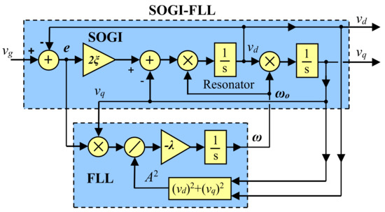
Figure 1.
Block diagram of the SOGI-FLL filter.
The SOGI has a second-order band-pass filter (BPF) and a low-pass filter (LPF) behavior for and [23], with the following transfer functions
The FLL is a gradient descent estimator [20,23], defined as
where is the estimate of the grid voltage amplitude, .
The linearized model of the SOGI-FLL in a quasi-locked operating point regarding the voltage amplitude and frequency is defined in [24,26,33], as (4) and (5), depicted in Figure 2.
where and are the frequency and amplitude of the grid voltage, respectively, and is the nominal value of the grid frequency, rad/s.
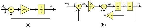
Figure 2.
Linearized models of the SOGI-FLL: (a) estimated voltage amplitude; (b) estimated voltage frequency.
The linearized models of (4) and (5) allow obtainment of the transient response of and for a sudden change in and , respectively, for a given value of and . The model of (4) is of a first-order system with constant time and, from linear control theory, it is well known that using an optimal relationship is achieved in the transient response of the system [1]. The model of (5) corresponds to a second-order system, whose transient response comes determined by the roots of (6):
In (6), it can be seen that and are related to the damping factor, , and natural undamped frequency, , respectively, in the standard definition of a second-order system, i.e., a system with roots . Then, by identifying and , it can be inferred that:
and extracting from the other identification:
and, putting (8) in (7) leads to:
Which choosing the optimal leads to a transient response that only relies on :
Then, by inserting these gains, and , in (6) gives roots located at , which corresponds to a transient response in that achieves an overshoot of and settling time , depicted in blue as the pair of gains in Figure 3.
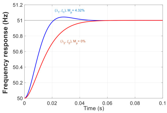
Figure 3.
Linearized response to a frequency step perturbation of 1 Hz for two sets parameters: (, ), in blue with and (, ), in red with .
By choosing this pair of gains, the transient response is optimal for the second-order system regarding achieved overshoot and settling time [1]. This, from the harmonic rejection point of view, it implies that a 3rd harmonic with a 3% amplitude voltage regarding nominal produces a ripple distortion around of 0.435 Hz, measured peak-to-peak. However, another interesting design point can be chosen instead for that corresponds to double real roots at , i.e., a transient response without overshoot, , since there are no imaginary parts in , see depicted in red as the pair in Figure 3. In this case, as the gain has been reduced by half, an extra attenuation to harmonics has been achieved and the ripple is reduced also by half, to 0.217 Hz. Notice that for the settling time is identical than for , since the real part of the roots for both gains are identical, i.e., . Therefore, we can consider as an optimal gain regarding harmonic-attenuation and . Additionally, this gain could be an interesting choice for those designers that are more interested in keeping the same but with an extra harmonic attenuation. From now on, in this paper, and are considered as two reference optimal gains for facing the perturbation induced by voltage sags and swells in the estimated frequency. The first one is better for achieving a faster transient response and the second one achieves a response with the same settling time but with better harmonic rejection capability.
Regarding the impact of voltage sags in the SOGI-FLL, the model in (4) can be used to obtain the transient response to the fault in the estimated grid voltage amplitude. But the model in (5) can provide the transient response of to a perturbation in the grid frequency, , but not to changes in since there are no-crossing terms between (4) and (5). Therefore, the impact in should be assessed using the real model depicted in Figure 1. Additionally, it is well known that the impact of voltage sags in the estimated is really high. Moreover, the transient response induced by the fault is nonlinear, and its magnitude size depends nonlinearly on the voltage sag’s depth, being worst for the deepest voltage sags.
Figure 4 provides an idea about the high impact of the perturbation induced in the estimated frequency by a voltage sag. Figure 4a depicts the estimated frequency for a series of voltage sags ranging from 0.8 pu to 0.2 pu for the optimal pair (, ). Figure 4b depicts the measured peak-to-peak value of the perturbation for each case. In this figure, the two pair of optimal gains, (, ) and (, ) had been considered. Notice that the size of the perturbation for can arrive to 15 Hz for the pair (, ) and of 6 Hz for (, ).
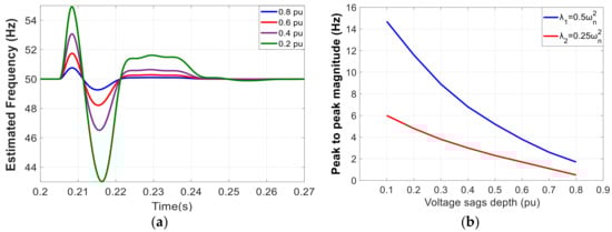
Figure 4.
(a) Estimated frequency perturbations in the SOGI-FLL for different voltage sag depths ranging from 0.8 pu to 0.2 pu and FLL gain . (b) Measured peak-to-peak maximum amplitude distortion in Hz, in blue for , in red for .
A similar impact, but with less peak-to-peak size, can be observed for a voltage swell in Figure 5a for voltage swells ranging from 1.2 to 1.8 pu and for the pair (, ). Additionally, Figure 5b depicts the measured peak-to-peak magnitude for the two pair of optimal gains, (, ) in blue and (, ) in red.
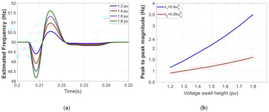
Figure 5.
(a) Estimated frequency perturbations in the SOGI-FLL for different voltage sag swells ranging from 1.2 to 1.8 pu and FLL gain . (b) Measured peak-to-peak maximum amplitude distortion in Hz, in blue for , in red for .
3. Reducing the Perturbation Impact by Means of a SOGI’s Error-Based Algorithm
The most effective approach for reducing the perturbation in the FLL estimated frequency is by means of using directly the error signal of the SOGI filter, because it receives directly the impact of the fault through the input voltage, i.e., . In this paper, a proposal is made using the error signal, the absolute value of the error signal, , and a low-pass filtering of , noted as and also as . The proposal consists in an algorithm that uses these variables as inputs and that provides a proper value of and to the SOGI-FLL for facing the fault and reduce the impact of the perturbation. This proposal is defined first for voltage sags and after is also applied to voltage swells. The block diagram that schematizes this proposal can be seen in Figure 6.
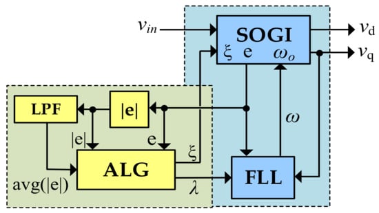
Figure 6.
SOGI-FLL-EbA proposal using e, and for reducing the impact of voltage sags and swells in the estimated frequency.
The algorithm is depicted in Figure 7 and is defined using only three states, named as S1, S2 and S3. From now on, the proposal will be named as SOGI-FLL “Error-based Algorithm”, SOGI-FLL-EbA. In the algorithm, S1 means normal operation. In this case, the SOGI-FLL-EbA operates with nominal gains (. This gains can be the pair () or (), but the pair () are used mainly in this paper. Then, at a fault event, spikes such as a sharp impulsive transient response. The error is compared to a given threshold and, if , the algorithm goes to state S2 were the SOGI-FLL-EbA runs with different gains named as (. These gains had been designed by a series of trial-and-error simulations for achieving a proper transient response and reduce the impact of the perturbation. The threshold is designed to be able respond to a frequency step change of ±2 Hz and to pass a harmonic distortion that can reach a 3% THD. The main objective had consisted into reducing the perturbation size to less than 2 Hz for the case of 0.2 pu, i.e., an 80% depth. To this purpose, the FLL gain, , has been strongly reduced.
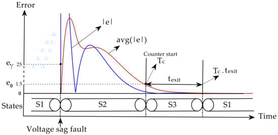
Figure 7.
SOGI-FLL-EbA using e, and signals for improving the frequency response in face of voltage sags and swells.
At this stage, the average input, is used for transitioning to S3. This average is obtained by using a LPF with a suitable cutoff frequency, , with the aim of filtering and generate an energy-like function for giving an indication of when the perturbation has passed over. The transitory of will consists in an impulsive function, see Figure 7 in red, that exponentially decays to zero, which, when is close to zero, means that the perturbation is over. Therefore, the algorithm goes to S3 only when is a given threshold, . Finally, a counter timer is started for giving a specific exit-time, . This counter helps to set a specific time delay to be performed before returning to state S1, in order to ensure a smooth returning to normal state. The exit-time is designed to cover all the different voltage sag depths. When the condition meets, the algorithm returns back to state S1 and the SOGI-FLL-EbA operates again with (.
Additionally, the same algorithm can be applied to voltage swells using e to identify a swell from a voltage sag. As , at the event of a fault, if means that the fault consists in a voltage sag and in a voltage swell. The gains (, threshold and exit time are different for voltage sags and swells and the values are depicted in Table 1.

Table 1.
SOGI-FLL-EbA parameters responding to voltage sags and swells.
4. Simulation and HIL Results
The SOGI-FLL-EbA proposal of Figure 6 has been discretized and simulated with Matlab/Simulink software. The SOGI-FLL-EbA gains during S1, S2 and S3 states and the thresholds , and exit-time are shown in Table 1. A third-order Adam–Bashforth method has been adopted, (11), for discretizing the SOGI filter following the discretization analysis performed in [34]. This method provides an exact −90° phase delay at the SOGI quadrature output and doesn’t have the drawbacks reported with backward, forward and trusting related methods, especially for low sampling frequencies.
and, the integrator of the FLL has been discretized using the backward Euler method:
Ts being the sample time of 100 µs, consistent with the 10 kHz frequency.
Figure 8a,b depicts the transient response of the SOGI-FLL and SOGI-FLL-EbA for a 0.2 pu voltage sag and 1.8 pu voltage swell, respectively. The faults happen at time 0.205 s. Notice how the perturbation in both cases had been reduced considerably, above 1 Hz peak-to-peak.
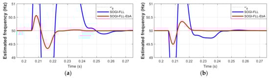
Figure 8.
SOGI-FLL and SOGI-FLL-EbA estimated frequency transient responses to 0.2 pu voltage sag and 1.8 pu voltage swell at 0.205 s, respectively.
The value chosen for the threshold has been designed to be able to accommodate a frequency step change of ±2 Hz and including a 3% THD harmonic distortion. Figure 9a depicts the transient response of the SOGI-FLL-EbA for a 2 Hz frequency step change at 0.2 s. Figure 9b shows the same transient response with a 3rd harmonic with 3% amplitude from nominal. Notice how the threshold allows the SOGI-FLL-EbA to respond to these perturbations, which do not trigger the proposed algorithm. It is important to remark that, since the “EbA” algorithm has not been triggered, these transient responses are identical to the achieved by a traditional SOGI-FLL, so they are not depicted in the figure.
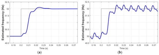
Figure 9.
Transient responses of the SOGI-FLL-EbA to a frequency step perturbation of 2 Hz. (a) without harmonic distortion. (b) with a 3rd harmonic and 3% voltage amplitude regarding nominal.
Figure 10 and Figure 11 depict the transient response of the SOGI-FLL and SOGI-FLL-EbA to voltage sags and swells with different durations. As fault transient, we consider here the event of a voltage sag or swell and recovery to nominal grid voltage in a short time. Fault events of Figure 10a extend for three and three quarters cycles while those in Figure 11a do so for three cycles and half. These responses show that the proposed algorithm reduces the impact of the perturbation and that allows a faster transient response. For this reason, Figure 10b and Figure 11b show the results for shorter fault lengths and have a contrast.
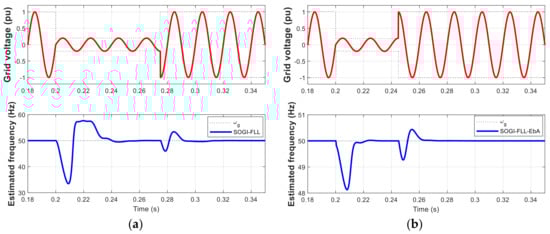
Figure 10.
Transient response of the SOGI-FLL and SOGI-FLL-EbA to short-duration voltage sags. (a) SOGI-FLL response to a 0.2 pu voltage sag at 0.2 s with three cycles and three quarters of duration. (b) SOGI-FLL-EbA response to 0.2 pu voltage sag at 0.2 s with two and half cycles of duration.
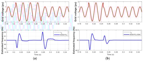
Figure 11.
Transient response of the SOGI-FLL and SOGI-FLL-EbA to short-duration voltage swell. (a) SOGI-FLL response to a 1.8 pu voltage swell at 0.205 s with three and half cycles of duration. (b) SOGI-FLL-EbA response to 1.8 pu voltage swell at 0.205 s with one and half cycles of duration.
Additionally, the grid voltage and the SOGI-FLL and SOGI-FLL-EbA had been implemented in a real-time HIL Typhoon 402 and HIL DSP100 platforms and the responses being captured in the typhoon SCADA panel [35]. Figure 12 shows the HIL results for the SOGI-FLL and SOGI-FLL-EbA to a periodic voltage sag fault transient that goes from 1 pu to 0.2 pu and then return back to 1 pu., the voltage sags go down to 0.2 pu and then return to 1 pu. In a similar way, Figure 13 depicts the transient results for a voltage swell that goes from 1 pu to 1.8 pu and back to 1 pu. As in the Simulink simulations, these HIL results show how the SOGI-FLL-EbA noticeably reduces the impact of the perturbation, allowing a faster response and respond to shorter duration transient faults.
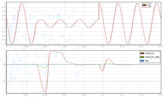
Figure 12.
HIL results for the SOGI-FLL and SOGI-FLL-EbA to short-duration voltage sag. (up) Grid voltage sag fault going from 1 pu to 0.2 pu and going back to 1 pu. (down) SOGI-FLL (red) and SOGI-FLL-EbA (green) estimated frequency response to the voltage sag in Hz.
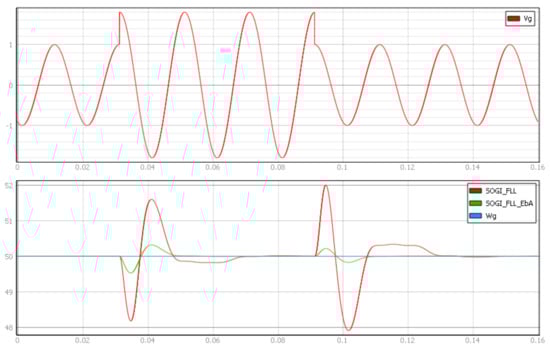
Figure 13.
HIL results for the SOGI-FLL and SOGI-FLL-EbA to short-duration voltage swell. (up) Grid voltage swell fault going from 1 pu to 1.8 pu and going back to 1 pu. (down) SOGI-FLL (red) and SOGI-FLL-EbA (green) estimated frequency response to the voltage sag in Hz.
Moreover, the peak-to-peak size of the perturbation had been measured for different depth and height sizes to assess the reduction in the perturbation achieved by the proposal using MATLAB/Simulink. Figure 14 depicts these measurements that show that the algorithm functions effectively in all the ranges defined for sags and swells.
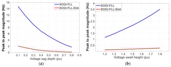
Figure 14.
Measured peak-to-peak maximum amplitude distortion in Hz for different voltage sags and swells. (a) For sags with depths ranging from 0.1 to 0.8 pu. (b) For swells with heights ranging from 1.2 to 1.8 pu.
5. Conclusions
This paper tried to improve the response of the SOGI-FLL to voltage sags and swells, since it is highly sensitive to these kinds of faults, especially to voltage sags. The paper first showed the scope of this problem for a given set of optimal SOGI-FLL gain parameters considered from the point of view of the SOGI-FLL’s optimal speed response to frequency step changes in the grid and of optimal capability rejection to harmonics. Then, it proposes an algorithm using the SOGI’s error signal and its absolute and average values for facing voltage sags and swells faults, reducing the impact in the estimated frequency. The MATLAB/Simulink simulations and real-time Typhoon HIL results showed the feasibility of this approach, which improved the response to these faults and reduced the recovery time involved in the transient perturbation.
Author Contributions
Investigation, simulation results, and writing—original draft, S.A.N. and J.M.; methodology and formal analysis, S.A.N., J.M., H.M. and J.d.l.H.; writing—review and editing, S.A.N., J.M., J.E., H.M. and J.d.l.H.; writing—response to reviewers, S.A.N., J.M., J.E., H.M. and J.d.l.H.; software design, S.A.N. and J.M.; data curation, S.A.N. and J.M.; organization and supervision, J.M., J.E. and J.d.l.H.; Tyhpoon HIL results, J.E. and J.M. All authors have read and agreed to the published version of the manuscript.
Funding
This research received no external funding.
Conflicts of Interest
The authors declare no conflict of interest.
References
- Ogata, K.; Brewer, J.W. Modern Control Engineering, 4th ed.; Prentice-Hall: Hoboken, NJ, USA, 2002. [Google Scholar]
- Dugan, R.C.; Mcgranaghan, M.F.; Santoso, S.; Beaty, H.W. Electrical Power Systems Quality, 3rd ed.; McGraw-Hill: New York, NY, USA, 2002. [Google Scholar]
- Kusko, A.; Thompson, M.C. Power Quality in Electrical Systems; McGraw-Hill: New York, NY, USA, 2007. [Google Scholar]
- Teodorescu, R.; Liserre, M.; Rodríguez, P. Grid Converters for Photovoltaic and Wind Power Systems; John Wiley & Sons: Hoboken, NJ, USA, 2011; Volume 29. [Google Scholar]
- IEEE Recommended Practices and Requirements for Harmonic Control in Electric Power Systems; IEEE Std 519-1992; IEEE: Piscataway, NJ, USA, 1993; pp. 519–1992.
- Matas, J.; Castilla, M.; Miret, J.; De Vicuna, L.G.; Guzman, R. An Adaptive Prefiltering Method to Improve the Speed/Accuracy Tradeoff of Voltage Sequence Detection Methods Under Adverse Grid Conditions. IEEE Trans. Ind. Electron. 2014, 61, 2139–2151. [Google Scholar] [CrossRef]
- Naidoo, R.; Pillay, P. A New Method of Voltage Sag and Swell Detection. IEEE Trans. Power Deliv. 2007, 22, 1056–1063. [Google Scholar] [CrossRef]
- Yunus, A.S.; Masoum, M.A.; Abu-Siada, A. Application of SMES to enhance the dynamic performance of DFIG during voltage sag and swell. IEEE Trans. Appl. Supercond. 2012, 22, 5702009. [Google Scholar] [CrossRef]
- Popavath, L.N.; Kaliannan, P. Photovoltaic-STATCOM with low voltage ride through strategy and power quality enhancement in a grid integrated wind-PV system. Electronics 2018, 7, 51. [Google Scholar] [CrossRef]
- Rey-Boué, A.B.; Guerrero-Rodríguez, N.F.; Stöckl, J.; Strasser, T.I. Modeling and Design of the Vector Control for a Three-Phase Single-Stage Grid-Connected PV System with LVRT Capability according to the Spanish Grid Code. Energies 2019, 12, 2899. [Google Scholar] [CrossRef]
- Safdarian, A.; Fotuhi-Firuzabad, M.; Lehtonen, M. A General Framework for Voltage Sag Performance Analysis of Distribution Networks. Energies 2019, 12, 2824. [Google Scholar] [CrossRef]
- Pu, Y.; Yang, H.; Ma, X.; Sun, X. Recognition of Voltage Sag Sources Based on Phase Space Reconstruction and Improved VGG Transfer Learning. Entropy 2019, 21, 999. [Google Scholar] [CrossRef]
- Li, D.; Mei, F.; Zhang, C.; Sha, H.; Zheng, J. Self-Supervised Voltage Sag Source Identification Method Based on CNN. Energies 2019, 12, 1059. [Google Scholar] [CrossRef]
- Serrano-Fontova, A.; Torrens, P.C.; Bosch, R. Power Quality Disturbances Assessment during Unintentional Islanding Scenarios. A Contribution to Voltage Sag Studies. Energies 2019, 12, 3198. [Google Scholar] [CrossRef]
- Chamchuen, S.; Siritaratiwat, A.; Fuangfoo, P.; Suthisopapan, P.; Khunkitti, P. High-Accuracy Power Quality Disturbance Classification Using the Adaptive ABC-PSO as Optimal Feature Selection Algorithm. Energies 2021, 14, 1238. [Google Scholar] [CrossRef]
- Doget, T.; Etien, E.; Rambault, L.; Cauet, S. A PLL-Based Online Estimation of Induction Motor Consumption Without Electrical Measurement. Electronics 2019, 8, 469. [Google Scholar] [CrossRef]
- Sun, Y.; De Jong, E.C.W.; Wang, X.; Yang, D.; Blaabjerg, F.; Cuk, V.; Cobben, J.F.G. The Impact of PLL Dynamics on the Low Inertia Power Grid: A Case Study of Bonaire Island Power System. Energies 2019, 12, 1259. [Google Scholar] [CrossRef]
- Du, H.; Sun, Q.; Cheng, Q.; Ma, D.; Wang, X. An Adaptive Frequency Phase-Locked Loop Based on a Third Order Generalized Integrator. Energies 2019, 12, 309. [Google Scholar] [CrossRef]
- Filipovic, F.; Petronijevic, M.; Mitrovic, N.; Bankovic, B.; Kostic, V. A Novel Repetitive Control Enhanced Phase-Locked Loop for Synchronization of Three-Phase Grid-Connected Converters. Energies 2020, 13, 135. [Google Scholar] [CrossRef]
- Rodríguez, P.; Luna, A.; Candela, I.; Mujal, R.; Teodorescu, R.; Blaabjerg, F. Multiresonant Frequency-Locked Loop for Grid Synchronization of Power Converters Under Distorted Grid Conditions. IEEE Trans. Ind. Electron. 2010, 58, 127–138. [Google Scholar] [CrossRef]
- Park, S.J.; Nguyen, T.H.; Lee, D.-C. Advanced SOGI-FLL scheme based on fuzzy logic for single-phase grid-connected con-verters. J. Power Electron. 2014, 14, 598–607. [Google Scholar] [CrossRef]
- Kang, J.W.; Shin, K.W.; Lee, H.; Kang, K.M.; Kim, J.; Won, C.Y. A Study on Stability Control of Grid Connected DC Distribution System Based on Second Order Generalized Integrator-Frequency Locked Loop (SOGI-FLL). Appl. Sci. 2018, 8, 1387. [Google Scholar] [CrossRef]
- Matas, J.; Martin, H.; de la Hoz, J.; Abusorrah, A.; Al-Turki, Y.A.; Al-Hindawi, M. A family of gradient descent grid frequency estimators for the SOGI filter. IEEE Trans. Power Electron. 2018, 33, 5796–5810. [Google Scholar] [CrossRef]
- Golestan, S.; Ebrahimzadeh, E.; Guerrero, J.M.; Vasquez, J.C. An Adaptive Resonant Regulator for Single-Phase Grid-Tied VSCs. IEEE Trans. Power Electron. 2018, 33, 1867–1873. [Google Scholar] [CrossRef]
- Matas, J.; Martin, H.; Elmariachet, J.; Abusorrah, A.; Al-Turki, Y. A New LPF-Based Grid Frequency Estimation for the SOGI Filter with Improved Harmonic Rejection. Renew. Energy Power Qual. J. 2018, 1, 716–721. [Google Scholar] [CrossRef]
- Golestan, S.; Guerrero, J.M.; Vasquez, J.C.; Abusorrah, A.M.; Al-Turki, Y. Modeling, Tuning, and Performance Comparison of Second-Order-Generalized-Integrator-Based FLLs. IEEE Trans. Power Electron. 2018, 33, 10229–10239. [Google Scholar] [CrossRef]
- Ye, S. Fuzzy sliding mode observer with dual SOGI-FLL in sensorless control of PMSM drives. ISA Trans. 2019, 85, 161–176. [Google Scholar] [CrossRef]
- El Mariachet, J.; Matas, J.; Martín, H.; Li, M.; Guan, Y.; Guerrero, J.M. A Power Calculation Algorithm for Single-Phase Droop-Operated-Inverters Considering Linear and Nonlinear Loads HIL-Assessed. Electronics 2019, 8, 1366. [Google Scholar] [CrossRef]
- Cao, W.; Liu, K.; Kang, H.; Wang, S.; Fan, D.; Zhao, J. Resonance Detection Strategy for Multi-Parallel Inverter-Based Grid-Connected Renewable Power System Using Cascaded SOGI-FLL. Sustainability 2019, 11, 4839. [Google Scholar] [CrossRef]
- Matas, J.; Martin, H.; De La Hoz, J.; Abusorrah, A.; Al-Turki, Y.A.; Alshaeikh, H. A New THD Measurement Method with Small Computational Burden Using a SOGI-FLL Grid Monitoring System. IEEE Trans. Power Electron. 2019, 35, 5797–5811. [Google Scholar] [CrossRef]
- Kim, D.-H.; Kim, M.-S.; Kim, H.-J. Frequency-Tracking Algorithm Based on SOGI-FLL for Wireless Power Transfer System to Operate ZPA Region. Electronics 2020, 9, 1303. [Google Scholar] [CrossRef]
- Nejad, S.A.; Matas, J.; Martín, H.; De La Hoz, J.; Al-Turki, Y.A. New SOGI-FLL Grid Frequency Monitoring with a Finite State Machine Approach for Better Response in the Face of Voltage Sag and Swell Faults. Electronics 2020, 9, 612. [Google Scholar] [CrossRef]
- Golestan, S.; Guerrero, J.M.; Vasquez, J.C.; Abusorrah, A.M.; Al-Turki, Y.A. Standard SOGI-FLL and Its Close Variants: Precise Modeling in LTP Framework and Determining Stability Region/Robustness Metrics. IEEE Trans. Power Electron. 2020, 36, 409–422. [Google Scholar] [CrossRef]
- Golestan, S.; Guerrero, J.M.; Musavi, F.; Vasquez, J.C. Single-Phase Frequency-Locked Loops: A Comprehensive Review. IEEE Trans. Power Electron. 2019, 34, 11791–11812. [Google Scholar] [CrossRef]
- Typhoon HIL. Hil 4/6 Series Hardware User Guide; Typhoon HIL Inc.: Somerville, MA, USA, 2021; Available online: https://www.typhoon-hil.com/documentation/typhoon-hil-hardware-manual/hil4-6_series_user_guide/topics/hil4-6_abstract.html (accessed on 10 June 2021).


Publisher’s Note: MDPI stays neutral with regard to jurisdictional claims in published maps and institutional affiliations. |
© 2021 by the authors. Licensee MDPI, Basel, Switzerland. This article is an open access article distributed under the terms and conditions of the Creative Commons Attribution (CC BY) license (https://creativecommons.org/licenses/by/4.0/).