Abstract
Electric vehicles are becoming more and more popular. One of the most promising possible solutions is one where a hybrid powertrain made up of a FC (Fuel Cell) and a battery is used. This type of vehicle offers great autonomy and high recharging speed, which makes them ideal for many industrial applications. In this work, three ways to build a hybrid power-train are presented and compared. To illustrate this, the case of an industrial robot designed to move loads within a fully automated factory is used. The analysis and comparison are carried out through different objective criteria that indicate the power-train performance in different battery charge levels. The hybrid configurations are tested using real power profiles of the industrial robot. Finally, simulation results show the performance of each hybrid configuration in terms of hydrogen consumption, battery and FC degradation, and dc bus voltage and current regulation.
1. Introduction
Electric vehicles (EV) are becoming a fundamental tool to face the problems introduced by the use of fossil fuels [1]. Currently there are different technologies and architectures for electric vehicles [2]. Today’s most predominant EV power-train is the one based only on rechargeable batteries as energy source, named Battery Electric Vehicles (BEV). The increasing availability of recharge stations and their home versions have provided a great scenario to BEV’s proliferation. The main drawback associated to BEV’s is its price and it reduced autonomy range. In this way, to increase the autonomy the capacity of the battery should be augmented and the price will be higher as a consequence [3]. In contrast, BEVs are simpler since they have a single energy source and a single energy storage system.
EVs can also have hybrid traction systems becoming Hybrid Electrical Vehicles (HEV), and be composed of different energy sources and have different energy storage systems. The combination of all these elements makes possible to improve the efficiency, autonomy range and the component lifetime of BEVs, but in return they require more complex energy management and control systems.
A first option, collected in the literature, is the traction system composed of batteries and super-capacitors [4,5]. This option makes it possible to take advantage of the batteries high-energy and the super-capacitors high-power density and thereby extend the battery lifetime in addition to being able to take better advantage of regenerative braking.
Hydrogen is becoming an ideal energy vector to help in the transition towards a cleaner and more sustainable energy system [6,7]. One of the fields in which hydrogen is beginning to excel is EVs. References [8,9], with the introduction of Fuel Cell Electrical Vehicles (FCEV). The use of hydrogen Fuel Cells (FC) in hybrid power-trains have gained major attention due its clean energy and satisfactory efficiency [10,11,12].
Nevertheless, there are still some issues on using a FC as part of the power-train. These issues regard performance and lifespan. The FC exhibits slow transient response which limits the performance under fast changing power profiles [13]. At the same time, fast power changes yield drops in pressure of the hydrogen stack, known as starvation, which in turn cause a rapid reduction of the cell voltage. This phenomena leads to premature degradation and eventually the damage of the FC [11]. To overcome this problem hybrid architectures are used. Hybridization advantages can be summarized as [14,15]:
- Handling pulses or fast variations in power demand, allowing improved acceleration profiles
- Providing larger power when both sources are acting together
- In case of FC failure, the vehicle can operate in a degraded mode.
- Allow the selection of smaller power components, thus decreasing the costs
- Regenerative breaking is possible
To hybridize the power-train an energy storage system is usually incorporated [16]. Commonly, this energy storage device is an electric battery [13], but it is also usual the use of a super-capacitor (SC) [17], or the combination of both [18,19,20]. The selection of the configuration depends on the concrete application. Moreover, economic aspects must be considered: considering the cost per unit of energy stored [17], batteries are a cheaper solution than SC, while these allow the handling of bigger power pulses without suffering degradation [21]. Sizing is also a very important problem that needs to be addressed in order to achieve a good trade-off between cost and performance [20,22].
The architecture of the hybrid power-train depends on the used electronic interfaces, typically DC-DC converters. Configurations can be classified as passive, semi-active or full-active. Selection of the most suitable configuration is highly important [23].
In this work, a hybrid power-train for an industrial mobile robot consisting of a hydrogen FC and a battery is considered. Four configurations for the power-train are studied and analysed: battery only, FC-battery in passive, a semi-active and a full-active hybrid topology. Each hybrid configuration is studied in terms of the characteristics and sizing of its components and the flexibility of the design. With this, provided advantages and drawbacks are defined taking into account the industrial robot requirements. As a base of comparison, different performance criteria are used. They include a battery degradation index, the fuel consumption and two quantitative FC degradation indicators. In the case of active hybrid configurations, current and voltage control loops are defined as well as an Energy Management System (EMS). All configurations are numerically tested using real power profiles from an industrial mobile robot. Constraints and characteristics of the robot, FC and battery are taken into account in order to analyse the performance of the system under selected configurations.
The paper is organized as follows: Section 2 describes the industrial mobile robot and its power profiles; Section 3 describes the considered performance criteria used for comparison purposes and provides quantitative indexes of FC degradation; Section 4 presents the four used configurations, the hydrogen FC and the battery; Section 5 shows the simulation setup and results, while Section 6 portrays the final conclusions.
2. The Industrial Mobile Robot
One type of vehicle that is currently on the rise, especially in the framework of Industry 4.0 [24,25], are industrial robots. Most of them are EV. For this reason, a device of this type has been selected to illustrate the developments of this work. In particular, it will be assumed that the analysed power-train feed the real consumption of an industrial robot.
The case study deals with a test robotic platform model Moby-500 (Steering Machines S.L., Bacelona, Spain). The machine, capable of moving a payload of up to 500 , has the dimensions shown in Figure 1. The platform features safety scanners capable of building a map of its environment, and is able to navigate safely using simultaneous localization and mapping (SLAM) technology. The platform is omnidirectional, employing conventional wheels and using a maximum of three motors to achieve any movement on a two-dimensional space.
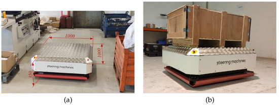
Figure 1.
(a) Moby-500 general view and dimensions (in millimeters), (b) Moby-500 with load.
The case studied correspond to maximum velocities of with a payload of 250 . The machine is ordered to travel along the edges of the two adjacent squares, as depicted in Figure 2. The tests are carried out in an industrial warehouse, with a floor featuring some irregularities. The circuit is divided into eight phases, each one covering one of the two-meter-long edges of one of the squares. For each phase, the platform starts from a static position and ends in a new static position that in turn becomes the starting point of the following phase. Therefore, each phase contains an initial acceleration segment and a final deceleration segment. Figure 3 shows the power consumption measured every 4 . From this, it can be gathered that each test entails eight consumption spikes.
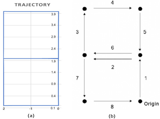
Figure 2.
Robot operation. (a) Trajectory calculated from internal odometry and (b) Sequence of movements.
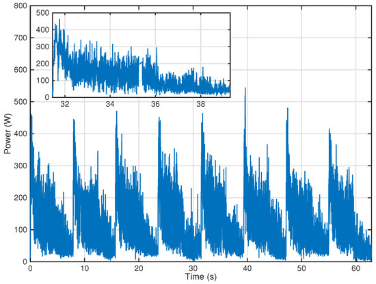
Figure 3.
Total power consumption of the robot as a function of time ().
3. Comparison Criteria
In order to compare and analyze the different power-train configurations and sizing for the mobile robot, different simulations will be carried out using Matlab-Simulink (Version 2019b, Mathworks, Natick, MA, United States). To do so, the generic battery and fuel cell models of Electrical Simscape Simulink Blockset will be used, with its parameters adjusted to each simulation. These models are quite generic, can be easily customized in size and technical characteristics, and have been used in many research papers [26,27].
The construction and design constrains of the different power-trains will be described when presenting each of the architectures. These restrictions include simplicity, the number of components, and their availability in the market.
Another area in which the different architectures will be compared is how they behave during the robot operation (using the consumption profiles described in the Section 2). In this context, the energy consumption will be analysed, both the variation of the energy stored in the battery and the hydrogen consumption (see Section 3.1) will be considered, and the degradation of the battery and the fuel cell will also be taken into account. Although degradation has a qualitative component, in order to carry out a degradation quantitative study, some indices that will be defined in Section 3.2 and Section 3.3, will be used.
3.1. Hydrogen Consumption
The rate at which hydrogen is consumed (in mol/s), , in a fuel cell is given by Faraday’s Law [10]:
where is the fuel cell current and F is the Faraday constant. can be also written in g/s as:
where is the hydrogen weight in g per mol.
On the other hand, it is common to provide flow rates of gases in liters per minute (lpm) and especially in standard liters per (slpm), where the standard liter is the quantity of gas that would occupy 1 L in standard conditions-atmospheric pressure, 101.3 kPa and 15 °C (in technical fluid mechanics standard temperature is 15 °C, not 25 °C as in chemistry) [10]. Thus, at standard conditions, molar volume is:
The volumetric hydrogen consumption rate in std lpm is given, then, by:
Joining Equations (2) and (4), we have the relationship between the flow rates at std lpm and the hydrogen consumed:
The fuel cell model used by MATLAB/Simulink [26] includes the calculation of hydrogen consumption from the fuel cell current described in this section.
3.2. Battery Degradation and Aging
Batteries are complex electrochemical devices. Their use is becoming popular, and extensive research is being carried out to improve the understanding of their operation. One of the main problems that has been the object of study, in recent years, is its useful life and the causes of its degradation [28,29,30]. The time of use is one of the determining factors of ageing, but the conditions in which the battery operates are also determining factors. In the latter, the architecture of the traction train can play a determining role.
In order to estimate the battery degradation, a method to quantify the damage produced in the battery by its usage is needed. Factors such as current severity (known as C-rate), elevate temperature, discharge rate or State of Charge (SOC), in addition to irregular patterns of charge and discharge cycles can accelerate battery degradation [31]. C-rate (defined for a given battery current) and depth of discharge (DOD, complementary to the battery SOC) are defined as:
where Q is the battery capacity expressed in Ah. High values of C-rate and of DOD tend to accelerate battery aging [13].
Following the strategy proposed in [13], the battery degradation will be estimated using the Ah-throughput parameter, as it takes into consideration both the current severity (either charge or discharge) and its DOD, as well as the battery working temperature. This accumulative parameter predicts the End of Life (EoL) of a battery when it exceeds a predetermined value, known as nominal Ah-throughput, where nominal conditions refer to a C-rate = 1, DOD = 100% and a temperature of 25 °C. This value, and the effective Ah-throughput that a current profile produces, are calculated as follows [13]:
where (t) is a weight factor bigger than 1 named severity factor, and it depends on the DOD and the operating temperature. It can be calculated using the severity factor map found in Figure 4 according to [31].
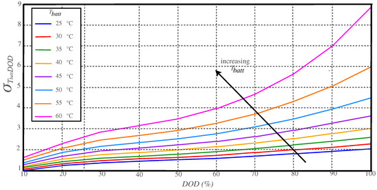
Figure 4.
Severity factor map depending on DOD and battery temperature.
As battery current is expected to be kept low, following the study in [32], the temperature of the battery can be estimated to be around 25 °C. Looking back at the severity factor map, and considering this temperature, three different severity zones have been defined:
- DOD = 1
- DOD = 1.2
- DOD = 1.5
No DOD values higher than 80% are considered, as it is considered that the battery is fully discharged when it reaches 20% SOC, as it is harmful for the battery life to operate under this limit.
3.3. Fuel Cell Degradation
Fuel cells are very efficient and clean devices [33,34]. Unfortunately, they continue to have significant degradation problems. Such degradation depends on ageing and many factors that depend on the operation of the device. In recent times, a very large scientific effort has been made to determine and characterize degradation main causes. Some of the main causes are poor water management (flooding or drying out) [35], reactants starvation [36,37], and the presence of contaminants in the fuel and in oxidant streams [38,39,40].
Fuel cells have two clearly differentiated parts, the fluid dynamic part and the electrical part. Although they are clearly coupled, the models commonly used to describe their behavior are very different in nature. The modelling and analysis of fluid dynamical phenomena is complex and requires sophisticated models that cannot usually be used in real time. In addition, the fluid dynamic part usually operates in closed-loop (i.e., a controller is automatically determining the value of most relevant variables). These controllers regulate the main variables of the system such as temperature, the amount of gases introduced, in addition to its temperature [41,42] and humidity [43,44]. With proper management it is possible to guarantee fluid-dynamic conditions that minimize the degradation of the fuel cell. In addition, although the fuel cell control system uses voltage and current information, it is usually independent of the power management system and therefore acts autonomously. This is especially relevant in commercial systems where the different components are manufactured by different companies.
The behavior of the electrical part is usually described using the polarization curve and the spectroscopy [10]. The first, provides the stationary behavior while the second provides information on dynamic one. The result of spectroscopy is usually a very interesting tool to characterize the health status of the fuel cell.
It is difficult to characterize the degradation of the fuel cell only from the point of view of the electrical part but there are electrical behaviors that contribute substantially to the degradation of the battery. The two main causes that we will consider in this work are
- High voltages. It is well known that working at voltages over degrades significantly the cell. It is convenient to take into account that these voltages are the ones which provide the best efficiency, so a trade-off between efficiency and degradation must be made when planning the power-flow.Many fuel-cell controllers disconnect the gas supply when they detect that there is no power consumption for a certain time in order to avoid that the open-circuit voltage, which is the one that degrades the most. Unfortunately, the start and stop processes also contribute significantly to the degradation and require a certain amount of time to be completed properly.In order to estimate the degradation due to high voltages the following index is proposed:where is the minimum voltage which produces degradation, in this work , and is the Heaviside function (i.e., 0 for and 1 for ). This index computes how many time the cell voltage has been over the reference value and how much the voltage has been over the reference.
- Fast load changes. Changes in the current must be accompanied by a change in the supply of gases in order to guarantee that the cell has the necessary amount of reactants. Since the fluid dynamics is, in general, slower than the electrical part, if there are sudden changes in the current it can happen that the gases have not reached all the parts of the cell. This phenomenon known as starvation induces a significant degradation in the fuel cell, therefore it is convenient that there are no sudden changes in the current.In order to estimate the degradation due to fast load changes the following index is proposed:where is the derivative threshold which might introduce degradation, in this work will be assumed.
4. Hybrid Power-Train Architectures
According to the literature, there exist many ways to combine a battery and a fuel cell, additionally it is possible to use, or not, power converters and passive elements such as inductors, capacitances or resistances. Each of these combinations defines a new architecture. In this section the most relevant ones will be presented and discussed.
4.1. Battery Only Powered Train
The simplest architecture is the one where the battery is used as the sole power source of the power-train. Although, this is not a hybrid system it will be used as reference to shown the benefits of using a hybrid system. Under this configuration, the battery current is equal to the load current. The robot autonomy can be calculated directly from the consumption profile data using the minimum SOC of the battery. The autonomy will depend on the battery capacity: the larger the capacity of the battery, the larger the autonomy of the robot. For this reason, this configuration is the less flexible one in terms of autonomy and efficiency.
4.2. Passive Hybrid Configurations
In passive configurations, a direct connection between the load, the battery and the fuel cell is found (see Figure 5). The connection point is usually named DC bus. Its immediate consequence is the need to carefully design and size its components in order to ensure a similar voltage range operation between the batteries and the FC [23]. The direct coupling of components makes that the voltage in the DC bus is set by the battery’s voltage. For this reason, a prior design of the battery is needed, as its nominal voltage has to be around the voltage of operation of the load. Moreover, the voltage of the battery depends on its SOC, and will decrease as the battery discharges. On the other hand, the fuel cell does not have an independent voltage, and its operating voltage only depends on the voltage set by the battery, as it is the one found in the DC bus where it is connected, and their relative impedance. Following its polarization curve, the FC will provide electric current for the given voltage. Thus, one of the main drawbacks of this architecture is that, the fuel cell and the battery do not necessarily work at its maximum efficiency, and dangerous operating conditions can occur [45]. Additionally, the lack of control can cause a degradation in the performance of the FC [45]. On the other hand, the advantages of passive configurations with respect to active ones are various. The simpler architecture leads to a lower risk of failure, as well as a lower weight and volume, and a reduced cost in general. Moreover, the absence of power converters lowers the system’s losses, leading to a higher overall efficiency. For these reasons, passive configurations can be a better option for lightweight vehicles, where the energy demand is lower and the hydrogen can be stored in low-pressure on-board storages of metal hydrides.
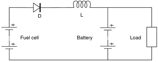
Figure 5.
Electric circuit schematic of a passive hybrid power system.
In Figure 5, the electric circuit of a passive hybrid power system can be seen. A diode is used to ensure a safe operation of the FC, as it avoids negative currents that would be harmful. An inductor can also be used to prevent rapid changes in the FC’s current, which would be harmful to its performance. The power demands of the load are handled by the battery and the fuel cell jointly. If the power required by the load is higher than the one provided by the FC, the battery will provide the extra power to meet the power demands, and if the power provided by the FC is higher than the required by the load, it will serve for both meeting the power requirements of the load and charging the batteries with the extra power. The inductor avoids fast variations of power demand in the FC, so it can provide almost constant power. This ensures a safe operation of the FC and premature degradation will be avoided. The equations that model this system are:
There are also several ways to implement a passive hybridization. For instance, several possible architectures can be found depending on whether the FC can recharge the batteries or not. In this work, only the case where the FC is able to recharge the batteries with its extra power will be studied, as the vehicle will have larger autonomy if the batteries can be recharged.
4.3. Active Hybrid Configurations
The main difference between active and passive hybrid configurations is the appearance of control elements (typically DC/DC boost converters). The battery and the FC are no longer coupled directly and can work on different voltages, meaning that the sizing and operating conditions of them can be designed independently. This allows a more precise control of the system power flow, thanks to the control and management of the converters. On the other hand, their main disadvantages are the opposite of the advantages of the passive configuration: a more complex system topology, a higher system weight, volume and cost and a reduced efficiency due to voltage losses [23].
Two different cases will be studied, the first where a DC/DC boost converter connects the fuel cells with the DC bus (it will be referred as “Semi-active” configuration), and a second case where, in addition to the first DC/DC converter, a second one, bidirectional in current, connects the batteries with the DC bus. It will be referred to as a “Full-active” configuration.
As the voltage in the FC is no longer fixed by the battery, an Energy Management Strategy (EMS) for the operating conditions of the fuel cells is needed. Different strategies to model the contribution of each power source in covering the power needs exist, depending on the objective followed. As the operating costs associated with hydrogen consumption represent a high percentage of the total cost, minimization of fuel consumption is one of the most common elections. Nevertheless, other criteria exist that also take into account the maximization of the vehicle’s autonomy or the lifetime of some of its components, as the battery or the fuel cell, that also represent a high percentage of the total costs when their life is relatively short [13]. One of the most widely used strategies is the Equivalent Consumption Minimization Strategy (ECMS) that takes into consideration the currents of the FC and the batteries. In general terms, the EMS selected should ensure the following [46]:
- Low hydrogen consumption
- High overall efficiency
- Long lifetime of components
In future sections the EMS selected for this work will be presented.
4.3.1. Semi-Active Hybrid Configuration
Figure 6 shows the assumed semi-active hybrid configuration, in it the battery is directly connected to the DC bus, while the FC is connected to it through a DC-DC boost converter. The DC bus voltage is fixed by the battery, as in the passive configuration. Nevertheless, this voltage is not the same voltage as the one working on the FC. The DC-DC boost converter acts as a step-up voltage converter, allowing the FC to work at lower voltage levels. The power flow in this configuration is described by the following equations:
where:
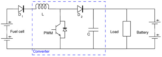
Figure 6.
Semi-active configuration schematic.
Once the operating point of the FC is set, the contribution of each power source is determined by Equations (14)–(16) [13]. As in the passive case, the fuel cell acts as the main power source and the battery complements it when needed. Like this, the FC can work with smooth profiles in order to avoid fast changing voltages that would be detrimental as it would cause starvation. FC and Battery will work together when the required power is higher than that of the FC and the FC will be used to provide power to the load and battery otherwise.
The introduction of the DC-DC converter allows the FC to work at more optimal voltage levels even if they are lower than the voltage of the batteries, as the converter will step its input voltage (FC’s voltage) up to the output voltage (DC bus voltage). Nevertheless, as the output power is smaller than the input one due to the converter efficiency, a higher output voltage leads to lower output current [47]. Equation (15) can be rewritten as:
In opposition to the passive configuration, where the operation of the FC was voltage-controlled (the voltage of the batteries fixed the voltage of the FC, and this one set its current through the polarization curves), in this configuration the FC can be current-controlled, as the FC can work at the desired current, fixing its voltage through the polarization curves.
4.3.2. Full-Active Hybrid Configuration
As can be seen in Figure 7, in the full-active hybrid configuration neither the battery nor the fuel cells are connected directly to the DC bus. The fuel cell, as in the case before, is connected through a unidirectional DC-DC boost converter that has the objective of stepping up the voltage of the FC to the DC bus voltage. In this case, in opposition to the semi-active architecture, the voltage of the DC bus can be controlled and does not depend on the voltage of the batteries, as a bidirectional DC-DC converter is placed between them. This converter differs from the one that connects the fuel cells to the DC bus in several aspects. Firstly, it is bidirectional in current, as it has to ensure current flowing from the battery to the load when the FC cannot cover the whole power of the load by itself, but also current from the DC bus to the battery, when the power provided by the FC is higher than the one required by the load and the batteries can recharge with the extra energy. In second place, the DC-DC converter is not of boost type, but of buck/boost, as it has either to step the voltage of the batteries up to the voltage of the DC bus when the batteries give power to the load or step the voltage of the DC bus down in the opposite case.
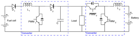
Figure 7.
Full-active hybrid configuration schematic.
The introduction of the DC-DC bidirectional converter allows a total control of the system and a total decoupling of its power elements with respect to the load. The control of the system is total because in addition to the variables controlled in the semi-active configuration, the voltage of the DC bus can be controlled through the current of the batteries and can be set to the desired value. Not only is the sizing of the FC decoupled from the battery’s design, but the battery is also independent of the load, as they no longer have to work at the same voltage. Nevertheless, it is important to consider the loss of battery current when it passes through the converter as its voltage is stepped-up, as it leads to an increase in battery’s consumption levels for equal load consumptions and a faster depletion of its SOC. For this reason, this type of architecture is not very common when a battery is the only ESS of the system, and is more usual when a supercapacitor acts as the main ESS of the system or as a complement to the battery [48].
A common bidirectional DC-DC converter is known as a Half-Bridge DC-DC converter, and is implemented through the connection in anti-parallel of a buck and a boost converter [49]. In Figure 7, a schematic of a Half-Bridge DC-DC Converter can be seen working between a low-voltage input source and a higher voltage output. Through the control of the time each switch is activated through PWM, the average output voltage value can be set for any value in between the upper and lower limits.
5. Simulation Results
5.1. Battery Only
Before entering in the analysis of the different power-train architectures, a study of the actual state of the robot’s power-train will be conducted. To do so, a simulation of the battery will be conducted. The battery has a capacity of 4000 mAh and works at 52 V which is the voltage needed by the motor driver of the real robot.
The Simulink circuit made to simulate the actual powertrain can be seen in Figure 8. It is a simple circuit where the load power profile of the industrial robot is used to generate the corresponding load current. The Simulink battery model give as output variables as SOC, current and voltage. As the battery is the only power source of the powertrain, it is expected that the load current will be equal to the one going through the battery.
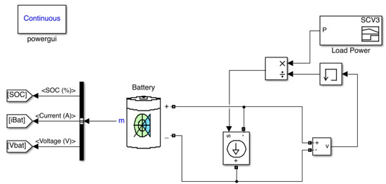
Figure 8.
Battery-only powertrain simulation circuit.
Two different simulations have been carried out, one at a high-SOC, which starts with a SOC level of 90%, and a second one at medium-SOC with initial level of 50%.
Figure 9 shows the evolution of the battery SOC, current, and voltage for the high-SOC scenario. As expected, the battery current is equal to the load current, as it is the sole power source of the vehicle. It can be seen current peaks produced by the planned motion of the robot. These current peaks generates the voltage ripple in the dc bus. The SOC, as expected, is decreasing continuously. In Figure 10, the results for medium-SOC conditions are shown. The overall behavior is similar to that of the high-SOC simulation, but noticing that the battery voltage is lower due to the inferior SOC level.
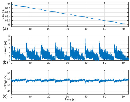
Figure 9.
Battery-only simulation results for high-SOC. (a) SOC, (b) battery current, (c) battery voltage.
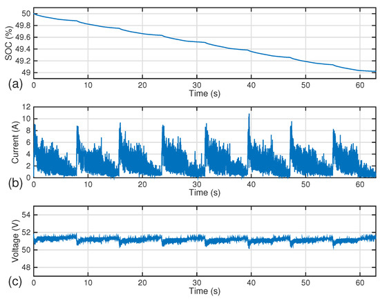
Figure 10.
Battery-only simulation results for medium-SOC. (a) SOC, (b) battery current, (c) battery voltage.
Additionally, relevant information related to this cycle can be seen in Table 1. It can be seen the maximum, minimum and mean values for the current and voltage variables; the maximum, minimum and the difference between initial and final values (Δ) for the SOC. Looking at Table 1, it is observed that the discharge rate, for the same current profile, is practically independent on the DOD of each case. How the lower voltage in the medium-SOC level causes small increments in current peaks compared to the high-SOC condition is also appreciated.

Table 1.
High and medium SOC battery-only simulation data.
With the data extracted from this simulation, an expected value of the robot’s actual autonomy can be calculated, given that its viable SOC range goes from 100% to 20%:
As can be seen, the autonomy of the robot is slightly greater than 1 h, which could be considered insufficient for the operational needs of the robot. The effective Ah-throughput is shown in Table 2. It can be seen that a larger is found in the medium-SOC case. This is due to the fact that for low values of SOC, the voltage of the Battery decreases and, since the power of the load remains constant, the load current increases.
Table 2.
Effective Ah-throughput for the battery-only simulation.
In the following sections, different powertrains will be tested with the objective of obtaining longer autonomy.
5.2. Passive Hybrid Powertrain
As seen in Section 4.2, the battery and the FC are directly coupled in the passive architecture. Its immediate consequence is the need to carefully design the fuel cell, as it has to be able to work at the voltage set by the batteries. The relation between the FC’s voltage and the one of the battery will depend on its relative impedance.
Two elements will be found between the battery and the FC: a diode to prevent negative currents entering the FC, and an inductor, as it will ensure that the FC operates without fast current changes, which would cause starvation and will harm the cell. Due to inductor high weight, the smallest inductor that ensures the FC’s safe operating conditions will be selected. After trying different inductor sizes, a value of mH has been selected.
Moving on to the sizing of the FC, it needs to be able to operate at similar voltage levels than the ones of the driver and battery, as they are the ones setting the DC bus’ voltage around 52 V. On the other side, the FC is designed to provide the average power of the load for the entire cycle. With all this, the FC should provide around 2.2 A to cover for the load needs. Figure 11 shows the fuel cell polarization curve.
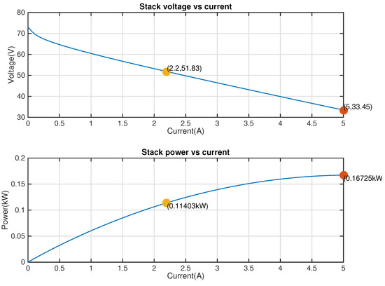
Figure 11.
Polarization curve of the FC for passive configuration.
The Simulink circuit made to simulate the passive hybrid power-train can be seen in Figure 12. It can be seen how the battery and fuel cell are directly coupled, with an inductor between them while the diode is included internally in the Simulink model of the FC.
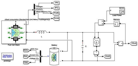
Figure 12.
Passive hybrid powertrain simulation circuit.
The power-train will be tested at three different SOC levels:
- High-SOC SOC = 90%
- Medium-SOC SOC = 50%
- Low-SOC SOC = 30%
Figure 13 shows the system response for the high-SOC passive hybrid simulation. It can be seen how the Battery starts and ends approximately at the same SOC percentage. This is a consequence of the FC selection, since it is designed to provide the averaged power of the load for this cycle, while the Battery is supplying the remaining demanded power. This effect is observed in the resulting current shape, where current peaks are provided by the Battery while an almost constant current is delivered by the FC. As a consequence of the passive configuration, FC and the Battery share the same voltage. Furthermore, this voltage is mainly defined by the Battery, showing small voltage drops that correspond to current peaks drawn by the load. Regarding the FC performance, as the operating point is almost constant, so are the efficiency and flow rate values.
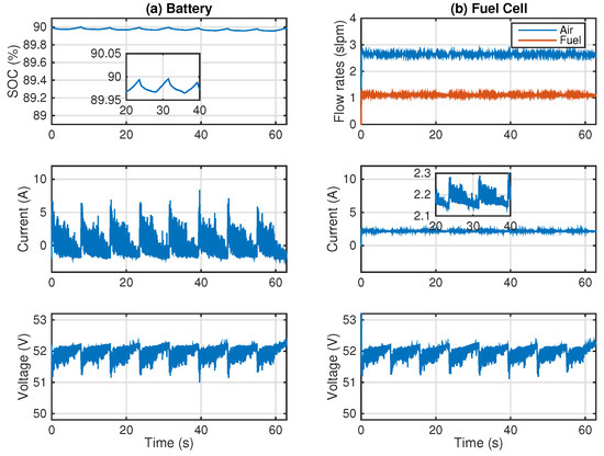
Figure 13.
High-SOC passive hybrid simulation. (a) Battery response, (b) FC response.
Simulations for medium and low SOC conditions are shown in Figure 14 and Figure 15, respectively. Very similar profiles to the ones seen in Figure 13 can be observed: the battery and FC work together to handle the load currents with almost constant FC current and the presence of peaks of current in the Battery. Once more, the Battery SOC ends at the same value it starts. The profiles seen in Figure 14 and Figure 15 show again almost constant values for the variables of the FC. However, the small differences are detailed below.
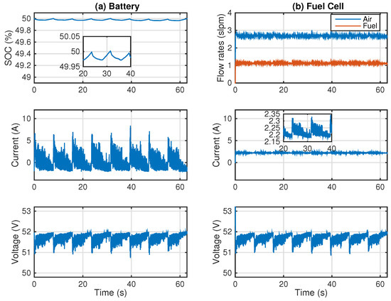
Figure 14.
Medium-SOC passive hybrid simulation. (a) Battery response, (b) FC response.
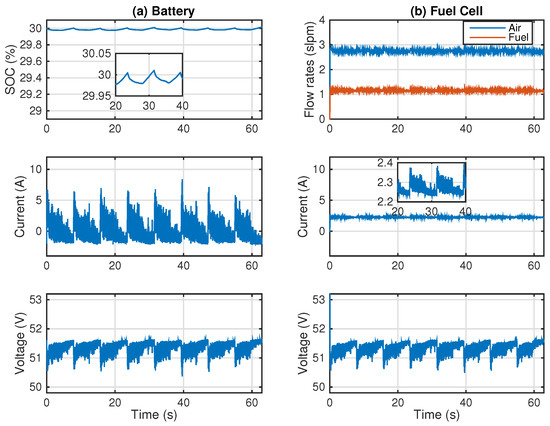
Figure 15.
Low-SOC passive hybrid simulation. (a) Battery response, (b) FC response.
A summary of the passive hybrid configuration information related to this cycle can be seen in Table 3 and Table 4. These data is relevant to compare the behavior of the passive configuration at different SOC levels.
Table 3.
Battery response in high, medium and low SOC passive hybrid simulation.
Table 4.
FC response in high, medium and low SOC passive hybrid simulation.
The information of the battery is shown in Table 4. The ΔSOC percentage comparison shows that at 50% SOC, the system is near to equilibrium: the initial and final Battery SOC can be considered the same. For high-SOC levels, the Battery is slightly discharged, while in low-SOC conditions it is charged. The current mean value also confirms this behavior, being positive at high-SOC, negative at low-SOC and almost 0 at 50% SOC. This means that, with the proposed design, the passive configuration will tend to a Battery SOC of 50%. Regarding battery voltage and current, the current has higher peaks as the SOC decreases, which is due to lower voltages at lower levels of SOC.
The FC data is in Table 4. As a lower SOC leads to lower voltage, the current contribution from the FC is higher when the SOC diminishes. Furthermore, the power supplied increases as the SOC is reduced. As predicted seeing the results of the battery performance, the current and power provided by the FC are slightly higher in expense of a little decrease in efficiency.
This means that with the correct sizing of the hydrogen storage system, any given autonomy can be achieved. Again, a decrease in battery voltage leads to a slightly higher FC current and power in expense of a little decrease in efficiency.
In order to compare with the other power-trains, in this section the control parameters, as hydrogen consumption or the effective Ah-throughput will be put together. They can be seen displayed in Table 5. It can be observed that operation at lower SOC the consumption is higher together with larger degradation of the battery and FC.
Table 5.
Performance parameters of the passive hybrid simulation.
On the qualitative performance aspects, this model has the positive aspect of making the FC work at almost constant operational levels. Voltage decreases at lower battery SOC, however, due to the proposed design, the system will tend to an equilibrium of 50% of SOC, allowing the FC and battery to operate in safe conditions. The autonomy will also depend on the hydrogen availability.
If a battery with lower capacity is used, the minimum values of the SOC are lower, the battery current peaks are larger and the voltage drops are deeper. The FC current will also present larger variations. All this together will increase the consumption and degradation of the battery and FC.
The degradation voltage index is zero in every case. This result indicates that the FC always work at voltages below the 85% percent of the FC open circuit voltage, which avoid its degradation. On the other hand, the current index shows some grade of affectation due to the current variations. The detailed picture of the FC current in Figure 13, Figure 14 and Figure 15, shows the small but rapid variations that cause the value of this index.
On the negative aspect of this configuration comes the sizing of the FC. The polarization curve defined does not belong to any commercial FC available. The voltage levels at which the cell has to work are really high when compared to its power. Low-power FCs are designed to work at around 12–18 V, in order to give acceptable levels of current. For this reason, even though passive hybrid configurations are a must-consider case in lightweight vehicles, it is not a viable option in this case as the sizing requirements do not match with any commercial fuel cells available.
5.3. Semi-Active Hybrid Configurations
The semi-active hybrid configuration overcomes the just commented FC voltage limitation of the passive one by implementing a DC-DC booster that steps the operating voltage of the FC up to the DC bus’ voltage. This allows the use of low-power fuel cells with relatively high DC bus voltages. As before, different FC sizes will be tested until achieving a point where the battery never gets depleted as long as hydrogen is supplied to the FC. In that case, any required autonomy can be achieved by correct sizing of the hydrogen storage system. In the opposite case, the autonomy of the vehicle would not only depend on the amount of hydrogen stored, as the battery could also be depleted before the hydrogen storage system empties.
As can be seen in the Simulink circuit displayed in Figure 16, the circuit incorporates several elements with respect to the passive one:
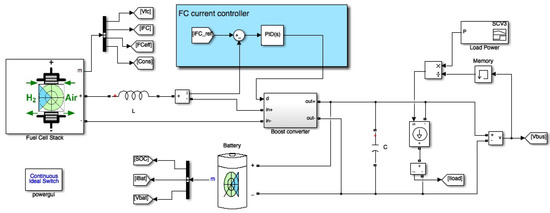
Figure 16.
Semi-active hybrid power-train simulation circuit.
- DC-DC Booster: consists of an inductor, a switching transistor, a diode and a capacitor.
- Active-control system: following the EMS selected, compares a reference value with the actual FC current, and through a PID controller gives a PWM signal to the switching transistor.
- Low-pass filter: filters the load power consumption in order to eliminate the high-frequency ripple and give a smoother current profile as FC current reference value.
The low-pass filter, which will remain constant for following sections and adjusted until reaching the desired degree of smoothness, has the following transfer function:
The intention is that the FC acts as the main power source and the battery complements the fast-changing current profiles in order to avoid starvation. Thus, the filtered current reference of the FC will be generated filtering the power at the load and then dividing by the FC voltage, that is, the power that the FC will provide is a filtered version of the load power. Figure 17 shows the block diagram of this operation.
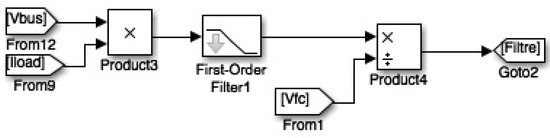
Figure 17.
Generation of the reference of the FC current: simulation block diagram.
Before entering in the simulation of the power-train at different SOC levels, the different components of the circuit need to be sized, and the control system designed. In this case, a FC with very similar power compared to the one used in the Passive configuration is used. However, the operational voltage of the FC is lower, as the FC will operate around 13–14 V and the DC bus voltage will be around 51–52 V, which is also the operational voltage of the battery. Its polarization curve can be seen in Figure 18.
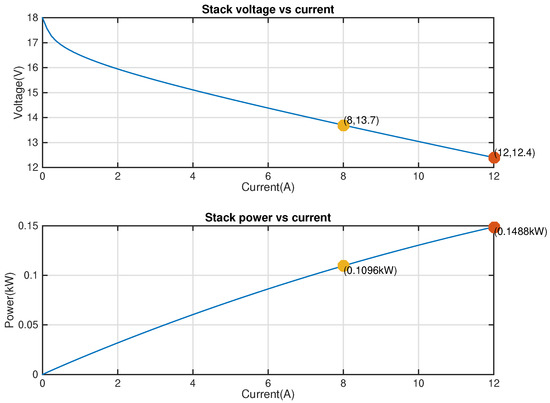
Figure 18.
Polarization curve of the FC for semi-active configuration.
Going on to the sizing of the DC-DC boost converter elements, the inductor’s size has been chosen as the minimum possible that ensures that no high current ripples appear in the FC. Similarly for the capacitor’s sizing, where a large capacitance value is needed in order to keep the voltage ripple low. Thus, the values for the elements conforming the DC-DC converter are and inductance L = 5 mH and capacitance C = 5000 μF.
Following the strategy found in [13], the Energy Management Strategy (EMS) followed has three different zones, depending on the battery SOC:
- SOC = 100–90% I = 0 (the vehicle runs on only battery)
- SOC = 90–40% I follows the filtered current
- SOC = 40–20% I = 10 (the FC runs at constant-power)
These three zones are achieved in the simulation through the block distribution shown in Figure 19.
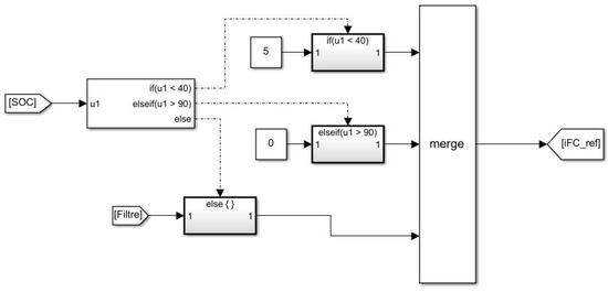
Figure 19.
Block distribution for the selection of the different EMS zones.
For low-SOC levels, the FC reference current was set to 10 A. This current supply the load consumption and prevent the batteries from being charged with large currents that could highly accelerate its degradation. Between 90%–40%, the FC reference current will be a filtered current. The objective of the middle EMS zone is to share the power of the load between the FC and the battery.
The last step before starting the simulation is the control system design. A PI controller will be selected to regulate the current of the FC, as the integral part is able to reduce the error in stationary state, which will be very effective when the reference current is constant (when the SOC of the battery is low), and the proportional part makes it adapt better when the reference current is variable. Without the proportional part, lots of noise appear in the FC signals. The values for the PI controller are adjusted to and .
As before, the power-train will be tested at three different SOC levels: high, medium and low, corresponding to 90%, 50%, and 30%, respectively
The simulation results for high-SOC for the semi-active hybrid configuration are shown in Figure 20. It can be seen that the battery operation is very similar to the passive case: voltage drops at currents peaks and a SOC that starts and ends at similar values. The big difference is appreciated in the FC behavior. With respect to the passive configuration, the FC current is higher and voltage is lower, as expected by the addition of the converter. Larger oscillations are also present in both FC current and voltage. Furthermore, the flow rates follow the oscillatory form of current and voltage. This is due to the low-pass filter used to generate the FC current reference. The actual filter bandwidth maintains the performance of the battery close to the one obtained in the passive configuration case. If a narrowed bandwidth is chosen, then the FC current and voltage oscillations will be smaller but the peaks in the battery current will be larger, causing larger voltage drops in the dc bus and more degradation of the battery. In this manner, the low-pass filter regulates the grade of hybridization of the system.

Figure 20.
High-SOC semi-active hybrid simulation. (a) Battery response and (b) FC response.
Figure 21 shows the results for the medium-SOC for the semi-active hybrid configuration. It shows similar profiles than the ones seen in the high-SOC case but with slightly lower battery voltage due to the reduced SOC. On the other hand, the FC performance is practically equal to the one obtained in the high-SOC case.

Figure 21.
Medium-SOC semi-active hybrid simulation. (a) Battery response and (b) FC response.
The simulation results for low-SOC can be seen in Figure 22. It shows how the FC is able to cover the load needs and charge the battery with extra power when providing a constant 10 A of current. As in this period the FC has been able to charge the batteries, it means that the battery will not be depleted while there is hydrogen available.
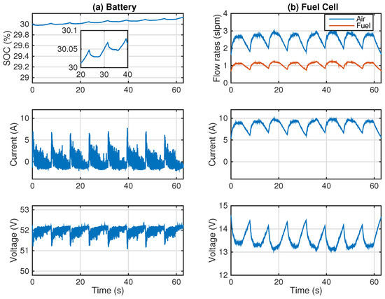
Figure 22.
Low-SOC semi-active hybrid simulation. (a) Battery response and (b) FC response.
The summary of the battery and FC relevant information related to this cycle is shown in Table 6 and Table 7, respectively.
Table 6.
Battery response in high, medium and low SOC semi-active hybrid simulation.
Table 7.
FC response in high, medium and low SOC semi-active hybrid simulation.
In Table 6, it is observed that for high and medium SOC, the current going through the battery and its ΔSOC remains very similar. Additionally, in Table 7, for these same SOC levels, the values obtained for the FC have no noticeable differences. This is due to the controller in the FC part, where the current reference is calculated from the power of the load, independently of the battery, and the PI controller rejects successfully the disturbances. Thus, using this configuration assures a very similar behavior in the zone defined by SOC = 90–40% despite of the SOC level. On the other hand, in the low-SOC level, due to the EMS strategy, the power provided by the FC is higher to cope the load demands and the battery charging process.
The parameters for performance evaluation for the semi-active configuration can be seen in Table 8.
Table 8.
Performance parameters of the semi-active hybrid simulation.
On the qualitative performance aspects, it can be said that the EMS selected and the control system adopted has allowed the FC to work following smooth profiles and within its reach, so safe operating conditions have been achieved. However, the use of this configuration has led to larger oscillations in the FC relevant signals. However, fuel consumption and degradation of components has decreased in the 40–90% SOC level and the battery is charged faster in low-SOC conditions. Additionally, the semi-active hybrid configuration overcomes the constructional problems presented in the passive configuration.
Specifically, compared to the passive configuration case, it can be seen that the hydrogen consumption has decreased between 6% and 5% approximately for high and medium SOC levels. Additionally, the Ah-throughput has decreased in a 5% when the vehicle is in power-shared mode (high and medium SOC levels).
When compared to the passive configuration, both the hydrogen consumption and the effective Ah-throughput have grown in the low-SOC zone. Although the increment is 7% in fuel consumption and 3% in the battery aging index, they can be considered moderately low having the advantage of a faster charge of the battery.
Regarding the FC degradation, the values obtained in the index, show that the FC operates safely below the given threshold. In case of the affectation by current rates, the index shows a lower degradation level compared to the passive configuration. This indicates that, though more oscillations are present in the FC current, its waveform has less high frequency changes.
For all these facts, and for the increased autonomy of the vehicle, this option can be considered a better one than battery-only and passive ones.
5.4. Full-Active Hybrid Configurations
The full-active hybrid configuration presents several advantages with respect to the semi-active configuration. On one hand, a total control is possible, as the voltage of the DC bus can be adjusted to the desired reference value. This allows a decoupling of the battery’s operating conditions with respect to the DC bus’ voltage. Like this, the voltage of the DC bus can be set to 52 V, the nominal operating voltage of the driver, and the battery can work at lower voltage levels. As it is a low-capacity battery, 5400 mAh, an operating voltage has been considered to be around 36 V.
For this configuration, the previous FC used in the semi-active case will be considered, as it has been shown that is powerful enough for the requirements of the load. In the full-active configuration, two DC-DC converters are found, which means that the battery will have to produce a higher current for the same load requirements, as it will get reduced in the converter.
As it can be seen in the Simulink circuit displayed in Figure 23, with respect to the semi-active case, the circuit incorporates a half-bridge converter between the battery and the DC bus. This converter is used to control the voltage of the DC bus. In this way, the desired voltage in the DC bus is achieved by adjusting the current given by the battery. To do that, the desired DC bus voltage (52 V) is compared with the actual one, and through a controller the reference battery current is generated, which in turn will be compared with the actual battery current, giving through another PI controller a PWM to the switching devices. This controller structure is shown in Figure 24. In the control system for the FC current, the same controller structure of the semi-active configuration is used, where the actual current is compared with a reference one and through a PI controller a PWM signal is given to the switching device.
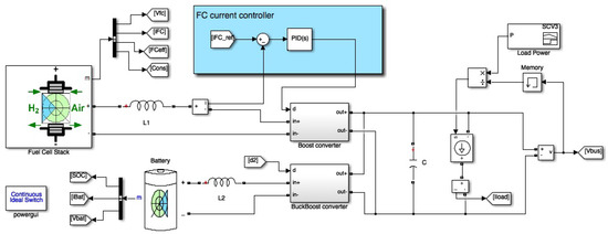
Figure 23.
Full-active hybrid powertrain simulation circuit.
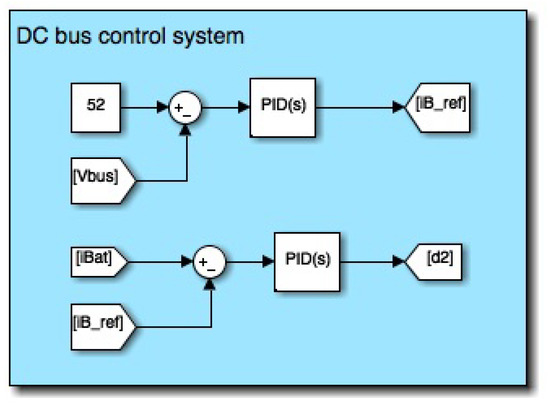
Figure 24.
DC bus control system simulation block diagram.
As the FC does not change, neither does the sizing of all its related components: the DC-DC boost converter sizing remains the same L = 5 mH and C = 5000 μF, and its control system will still be a PI controller. The EMS selected will be the same, and the reference current for the FC will still be the filtered version produced by the treatment of the load power (see Figure 17). Moving on to the sizing of the battery related components of dc-dc converter an inductance of 5mH is selected.
The last step before starting the simulation is the battery control system’s sizing, where two different controllers are needed. As before, PI controllers will be selected, as the integral part is able to reduce the error in stationary state, and the proportional part makes it adapt quicker. The values of the controller for the dc bus are and while the values for the battery current loop are and .
As before, the power-train will be tested at three different SOC levels: high, medium and low.
Simulation results for high and medium SOC levels are shown in Figure 25 and Figure 26. The performance of the FC is very similar to the one obtained in the semi-active configuration, as the same FC and controller is used in this part. The battery SOC initial and final value are almost the same. However, the currents peaks of the battery are larger than those of the previous configurations. This is a consequence of using a reduced voltage battery together with its associated DC-DC converter. In this way, if the output current of the half-bridge converter needs to cover for the remaining requirements of the load, the current that the battery needs to generate is higher, as increasing its voltage will cause a decrease in the current. It can also be observed, that he FC and battery performance is very similar between the medium and high-SOC case.
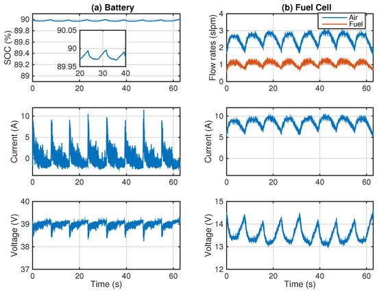
Figure 25.
High-SOC full-active hybrid simulation. (a) Battery response and (b) FC response.
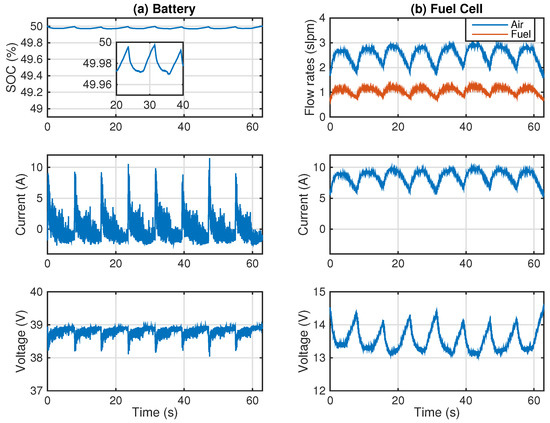
Figure 26.
Medium-SOC full-active hybrid simulation. (a) Battery response and (b) FC response.
The FC and battery performance at low-SOC can be seen in Figure 27. Thus, when the system is in the low-SOC zone, and extra current is used to charge the batteries, which flows through the bidirectional converter. With the design proposed, the current arriving to the battery causes almost the same charge speed than in the semi-active configuration.
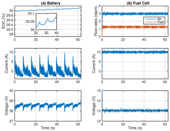
Figure 27.
Low-SOC full-active hybrid simulation. (a) Battery response and (b) FC response.
The battery and FC relevant information related to this cycle can be seen in Table 9 and Table 10, respectively. As in the semi-active case, with this configuration the behavior obtained in the zone defined by SOC = 90–40% is practically the same despite of the SOC level; and in the low-SOC level, the EMS makes the FC deliver more power to cope the load demands and the battery charging process.
Table 9.
Battery response in high, medium and low SOC full-active hybrid simulation.
Table 10.
FC response in high, medium and low SOC full-active hybrid simulation.
On the other hand, the evolution of the voltage of the DC bus can be seen in Figure 28 and its main information in Table 11. Although the mean voltage is around 52 V, it has larger voltage ripple compared to all previous configurations. However, the bus voltage regulation has improved significantly, obtaining almost the same voltage values despite the SOC level. This is due to the voltage controller. On the other hand, the ripple can be reduced using higher capacity capacitors and augmenting the PI gains in the voltage controller. However, in general, larger capacitors imply more weight and larger PI gains can lead to excessive high bandwidth, thus amplifying noise and reducing the robustness of the system.
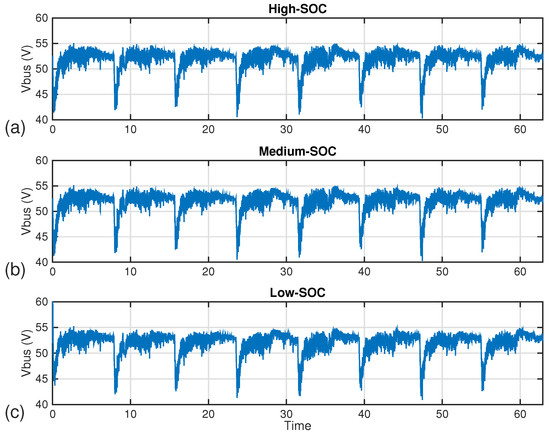
Figure 28.
Evolution of the voltage of the DC bus in (a) high, (b) medium, and (c) low SOC full-active hybrid simulation.
Table 11.
DC bus’s controlled voltage response in high, medium, and low SOC full-active hybrid simulation.
The evaluation parameters can be seen displayed in Table 12. On the qualitative performance aspects, as the performance of the FC has been the same than in the semi-active case, there are no differences with respect to that case, and the FC still has operated under safe conditions. Furthermore, with the introduction of the voltage of the DC bus controller, the voltage level has been kept regulated around 52 V disregarding the SOC level, although larger voltage ripple have appeared.
Table 12.
Performance parameters of the full-active hybrid simulation.
Comparing it to the results of the FC in semi-active configuration, it can be seen that the hydrogen consumption is the same for both configurations. However, the introduction of the bidirectional converter has increased substantially the battery degradation: the effective Ah-throughput has suffered an increase between 20% and 30%, approximately. This is a consequence of delivering the same power with a lower voltage battery.
The index indicates that there is no degradation in the FC due to the voltage level operation. If a different threshold is used, for example , the FC degradation index would be higher for high and medium SOC ( for high and medium SOC compared to in low-SOC), which is when voltage oscillations are present. However, the voltage oscillations do not surpass 0.85 and no real FC degradation occurs. On the other hand, the index demonstrates that, although the overall waveform of the FC current in this configuration is very similar to one obtained in the semi-active case, there are more high frequency components on it. An example of this type of degradation is due to the switching devices, where high frequency current ripple is present.
6. Discussion
In this section, the final conclusions regarding the comparisons between the powertrains performances will be presented. To do so, the different models will be referred as:
- Passive configuration PA
- Semi-active configuration SA
- Full-active configuration FA
The selection will be carried out using the criteria presented in Section 3 and Section 3.3, regarding constructive aspects, such as availability or component degradation, and performance aspects, such as fulfillment of requirements or hydrogen consumption. Initially, a comparison of the performance parameters is made in Table 13.
Table 13.
Comparison of performance parameters hybrid configurations.
It can be seen that the best performance is given by the semi-active configuration, with low consumption and battery degradation rates, as well as controllable autonomy, as its battery would only fully deplete if its FC ran out of hydrogen supply. The full-active configuration presents the same low consumption of the semi-active model, but larger battery degradation. This is a consequence of decreasing the working voltage of the battery thus obtaining higher currents. However, the bus voltage regulation can be improved in case of the full-active configuration.
Although active models increase the fuel consumption at low-SOC levels, they provide the characteristic of a faster charging of the battery.
Nevertheless, the decision does not just rely on the performance aspects, as the chosen configuration needs to ensure that it can be build and that it fulfills the necessary requirements.
As has been discussed in the respective sections, the passive model cannot be implemented because the integration of its elements is not possible, as the FC needed has a voltage range that can only be found in powerful FCs, making it both an unnecessary higher investment, and battery’s impossibility to deal with the high currents generated by the FC. On the other hand, the SA and FA models may accomplish the autonomy requirements with available FC.
As has been mentioned, the passive model might not be implemented as the FC needed has a voltage range that can only be found in powerful FCs, making it both an unnecessary higher investment, and battery’s impossibility to deal with the high currents generated by the FC at charging states. On the other hand, the SA and FA models may accomplish the autonomy requirements with available FCs.
The FA presents disadvantages with respect to its SA counterpart. Its battery degradation is higher and it presents added system complexity with more elements which lead to a higher cost, weight and volume. Its main advantages are the ability to adapt a low-voltage battery to a higher-voltage environment and better regulation of the bus voltage.
Finally, an additional characteristic of the active configurations is the flexibility regarding the hybridization of the system. It is carried out by means of the converter controllers and the EMS. Therefore, with active configurations there is the possibility of adding control schemes and an EMS that can be used to accomplish objectives of optimization and efficiency.
Author Contributions
Conceptualization, R.C.-C. and T.M.d.P.-C.; methodology, R.C.-C.; software, G.A.R.; validation, G.A.R., C.D.-M. and T.M.d.P.-C.; formal analysis, R.C.-C., T.M.d.P.-C., and G.A.R.; investigation, R.C.-C. and G.A.R.; resources, R.C.-C. and C.D.-M.; data curation, C.D.-M.; writing—original draft preparation, G.A.R., T.M.d.P.-C., and R.C.-C.; writing—review and editing, R.C.-C. and G.A.R.; visualization, R.C.-C.; supervision, R.C.-C.; project administration, R.C.-C.; funding acquisition, R.C.-C. All authors have read and agreed to the published version of the manuscript.
Funding
This research was supported by the María de Maeztu Seal of Excellence to IRI (ref. MDM-2016-0656) and the Spanish Ministry of Economy and Competitiveness under Project DOVELAR (ref. RTI2018-096001-B-C32).
Data Availability Statement
All simulation codes and used data are available upon demand to the authors.
Conflicts of Interest
The authors declare no conflict of interest.
References
- Nanaki, E.A.; Koroneos, C.J. Climate change mitigation and deployment of electric vehicles in urban areas. Renew. Energy 2016, 99, 1153–1160. [Google Scholar] [CrossRef]
- Sabri, M.M.; Danapalasingam, K.; Rahmat, M. A review on hybrid electric vehicles architecture and energy management strategies. Renew. Sustain. Energy Rev. 2016, 53, 1433–1442. [Google Scholar] [CrossRef]
- Delucchi, M.A.; Lipman, T.E. Lifetime Cost of Battery, Fuel-Cell, and Plug-in Hybrid Electric Vehicles; Elsevier B.V.: Amsterdam, The Netherlands, 2010; pp. 19–60. [Google Scholar]
- Paul, T.; Mesbahi, T.; Durand, S.; Flieller, D.; Uhring, W. Sizing of Lithium-Ion Battery/Supercapacitor Hybrid Energy Storage System for Forklift Vehicle. Energies 2020, 13, 4518. [Google Scholar] [CrossRef]
- Karangia, R.; Jadeja, M.; Upadhyay, C.; Chandwani, H. Battery-supercapacitor hybrid energy storage system used in Electric Vehicle. In Proceedings of the 2013 International Conference on Energy Efficient Technologies for Sustainability, Nagercoil, India, 10–12 April 2013; pp. 688–691. [Google Scholar] [CrossRef]
- Yue, M.; Lambert, H.; Pahon, E.; Roche, R.; Jemei, S.; Hissel, D. Hydrogen energy systems: A critical review of technologies, applications, trends and challenges. Renew. Sustain. Energy Rev. 2021, 146, 111180. [Google Scholar] [CrossRef]
- Cecilia, A.; Carroquino, J.; Roda, V.; Costa-Castelló, R.; Barreras, F. Optimal Energy Management in a Standalone Microgrid, with Photovoltaic Generation, Short-Term Storage, and Hydrogen Production. Energies 2020, 13, 1454. [Google Scholar] [CrossRef]
- Manoharan, Y.; Hosseini, S.E.; Butler, B.; Alzhahrani, H.; Senior, B.T.F.; Ashuri, T.; Krohn, J. Hydrogen Fuel Cell Vehicles; Current Status and Future Prospect. Appl. Sci. 2019, 9, 2296. [Google Scholar] [CrossRef]
- Bethoux, O. Hydrogen Fuel Cell Road Vehicles: State of the Art and Perspectives. Energies 2020, 13, 5843. [Google Scholar] [CrossRef]
- Frano, B. PEM Fuel Cells: Theory and Practice; Elsevier B.V.: Amsterdam, The Netherlands, 2005. [Google Scholar] [CrossRef]
- Roda, V.; Carroquino, J.; Valiño, L.; Lozano, A.; Barreras, F. Remodeling of a commercial plug-in battery electric vehicle to a hybrid configuration with a PEM fuel cell. Int. J. Hydrog. Energy 2018. [Google Scholar] [CrossRef]
- EG&G Technical Services. Fuel Cell Handbook, 7th ed.; National Energy Technology Laboratory: Morgantown, WV, USA, 2004. [Google Scholar] [CrossRef]
- Carignano, M.; Roda, V.; Costa-Castello, R.; Valino, L.; Lozano, A.; Barreras, F. Assessment of Energy Management in a Fuel Cell/Battery Hybrid Vehicle. IEEE Access 2019, 7, 16110–16122. [Google Scholar] [CrossRef]
- Kendall, K.; Shang, N.J. Hydrogen Utilization: Benefits of Fuel Cell—Battery Hybrid Vehicles; Elsevier B.V.: Amsterdam, The Netherlands, 2020. [Google Scholar]
- Thounthong, P.; Raël, S. The benefits of hybridization: An investigation of fuel cell/battery and fuel cell/supercapacitor hybrid sources for vehicle applications. IEEE Ind. Electron. Mag. 2009, 3, 25–37. [Google Scholar] [CrossRef]
- Chan, C.C.; Bouscayrol, A.; Chen, K. Electric, Hybrid, and Fuel-Cell Vehicles: Architectures and Modeling. IEEE Trans. Veh. Technol. 2010, 59, 589–598. [Google Scholar] [CrossRef]
- Carignano, M.G.; Costa-Castelló, R.; Roda, V.; Nigro, N.M.; Junco, S.; Feroldi, D. Energy management strategy for fuel cell-supercapacitor hybrid vehicles based on prediction of energy demand. J. Power Sources 2017, 360, 419–433. [Google Scholar] [CrossRef]
- García, P.; Fernández, L.M.; Torreglosa, J.P.; Jurado, F. Operation mode control of a hybrid power system based on fuel cell/battery/ultracapacitor for an electric tramway. Comput. Electr. Eng. 2013, 39, 1993–2004. [Google Scholar] [CrossRef]
- Li, H.; Ravey, A.; N’Diaye, A.; Djerdir, A. A novel equivalent consumption minimization strategy for hybrid electric vehicle powered by fuel cell, battery and supercapacitor. J. Power Sources 2018, 395, 262–270. [Google Scholar] [CrossRef]
- Sampietro, J.L.; Puig, V.; Costa-Castelló, R. Optimal Sizing of Storage Elements for a Vehicle Based on Fuel Cells, Supercapacitors, and Batteries. Energies 2019, 12, 925. [Google Scholar] [CrossRef]
- Wang, Y.; Sun, Z.; Chen, Z. Development of energy management system based on a rule-based power distribution strategy for hybrid power sources. Energy 2019, 175, 1055–1066. [Google Scholar] [CrossRef]
- Feroldi, D.; Carignano, M. Sizing for fuel cell/supercapacitor hybrid vehicles based on stochastic driving cycles. Appl. Energy 2016, 183, 645–658. [Google Scholar] [CrossRef]
- López González, E.; Sáenz Cuesta, J.; Vivas Fernandez, F.J.; Isorna Llerena, F.; Ridao Carlini, M.A.; Bordons, C.; Hernandez, E.; Elfes, A. Experimental evaluation of a passive fuel cell/battery hybrid power system for an unmanned ground vehicle. Int. J. Hydrog. Energy 2019, 44, 12772–12782. [Google Scholar] [CrossRef]
- Belman-Lopez, C.E.; Jiménez-García, J.A.; Hernández-González, S. Comprehensive analysis of design principles in the context of Industry 4.0. Rev. Iberoam. Autom. Inf. Ind. 2020, 17, 432–447. [Google Scholar] [CrossRef]
- Herrero, R.D.; Martínez, P.L.; Zorrilla, M. Reference architecture for the design and development of applications for Industry 4.0. Rev. Iberoam. Autom. Inf. Ind. 2021. [Google Scholar] [CrossRef]
- Motapon, S.N.; Tremblay, O.; Dessaint, L.A. Development of a generic fuel cell model: Application to a fuel cell vehicle simulation. Int. J. Power Electron. 2012, 4, 505–522. [Google Scholar] [CrossRef]
- Saw, L.; Somasundaram, K.; Ye, Y.; Tay, A. Electro-thermal analysis of Lithium Iron Phosphate battery for electric vehicles. J. Power Sources 2014, 249, 231–238. [Google Scholar] [CrossRef]
- Omar, N.; Firouz, Y.; Gualous, H.; Salminen, J.; Kallio, T.; Timmermans, J.; Coosemans, T.; Van den Bossche, P.; Van Mierlo, J. 9—Aging and degradation of lithium-ion batteries. In Rechargeable Lithium Batteries; Franco, A.A., Ed.; Woodhead Publishing Series in Energy; Woodhead Publishing: Cambridge, UK, 2015; pp. 263–279. [Google Scholar] [CrossRef]
- Grolleau, S.; Delaille, A.; Gualous, H. Predicting lithium-ion battery degradation for efficient design and management. World Electr. Veh. J. 2013, 6, 549–554. [Google Scholar] [CrossRef]
- Millner, A. Modeling Lithium Ion battery degradation in electric vehicles. In Proceedings of the 2010 IEEE Conference on Innovative Technologies for an Efficient and Reliable Electricity Supply, Waltham, MA, USA, 27–29 September 2010; pp. 349–356. [Google Scholar] [CrossRef]
- Onori, S.; Spagnol, P.; Marano, V.; Guezennec, Y.; Rizzoni, G. A new life estimation method for lithium-ion batteries in plug-in hybrid electric vehicles applications Pierfrancesco Spagnol Vincenzo Marano Yann Guezennec and Giorgio Rizzoni. Int. J. Power Electron. 2012, 4, 302–319. [Google Scholar] [CrossRef]
- Wang, P.; Yang, L.; Wang, H.; Tartakovsky, D.M.; Onori, S. Temperature estimation from current and voltage measurements in lithium-ion battery systems. J. Energy Storage 2021, 34, 102133. [Google Scholar] [CrossRef]
- Sorrentino, A.; Sundmacher, K.; Vidakovic-Koch, T. Polymer Electrolyte Fuel Cell Degradation Mechanisms and Their Diagnosis by Frequency Response Analysis Methods: A Review. Energies 2020, 13, 5825. [Google Scholar] [CrossRef]
- Liu, H.; Chen, J.; Hissel, D.; Lu, J.; Hou, M.; Shao, Z. Prognostics methods and degradation indexes of proton exchange membrane fuel cells: A review. Renew. Sustain. Energy Rev. 2020, 123, 109721. [Google Scholar] [CrossRef]
- Cecilia, A.; Serra, M.; Costa-Castelló, R. Nonlinear adaptive observation of the liquid water saturation in polymer electrolyte membrane fuel cells. J. Power Sources 2021, 492, 229641. [Google Scholar] [CrossRef]
- Liu, H.; Chen, J.; Hissel, D.; Hou, M.; Shao, Z. A multi-scale hybrid degradation index for proton exchange membrane fuel cells. J. Power Sources 2019, 437, 226916. [Google Scholar] [CrossRef]
- Ahmadi, P.; Torabi, S.H.; Afsaneh, H.; Sadegheih, Y.; Ganjehsarabi, H.; Ashjaee, M. The effects of driving patterns and PEM fuel cell degradation on the lifecycle assessment of hydrogen fuel cell vehicles. Int. J. Hydrog. Energy 2020, 45, 3595–3608. [Google Scholar] [CrossRef]
- Daeichian, A.; Ghaderi, R.; Kandidayeni, M.; Soleymani, M.; Trovão, J.P.; Boulon, L. Online characteristics estimation of a fuel cell stack through covariance intersection data fusion. Appl. Energy 2021, 292, 116907. [Google Scholar] [CrossRef]
- Chen, H.; Pei, P.; Song, M. Lifetime prediction and the economic lifetime of Proton Exchange Membrane fuel cells. Appl. Energy 2015, 142, 154–163. [Google Scholar] [CrossRef]
- de Bruijn, F.A.; Dam, V.A.T.; Janssen, G.J.M. Review: Durability and Degradation Issues of PEM Fuel Cell Components. Fuel Cells 2008, 8, 3–22. [Google Scholar] [CrossRef]
- Xing, Y.; Costa-Castelló, R.; Na, J. Temperature Control for a Proton-Exchange Membrane Fuel Cell System with Unknown Dynamic Compensations. Complexity 2020, 2020, 8822835. [Google Scholar] [CrossRef]
- Strahl, S.; Costa-Castelló, R. Model-based analysis for the thermal management of open-cathode proton exchange membrane fuel cell systems concerning efficiency and stability. J. Process Control 2016, 47, 201–212. [Google Scholar] [CrossRef]
- Luna, J.; Costa-Castelló, R.; Strahl, S. Chattering free sliding mode observer estimation of liquid water fraction in proton exchange membrane fuel cells. J. Frankl. Inst. 2020, 357, 13816–13833. [Google Scholar] [CrossRef]
- Cecilia, A.; Costa-Castelló, R. High gain observer with dynamic deadzone to estimate liquid water saturation in PEM fuel cells. Rev. Iberoam. Autom. Inf. Ind. 2020, 17, 169–180. [Google Scholar] [CrossRef]
- Di Trolio, P.; Di Giorgio, P.; Genovese, M.; Frasci, E.; Minutillo, M. A hybrid power-unit based on a passive fuel cell/battery system for lightweight vehicles. Appl. Energy 2020, 279, 115734. [Google Scholar] [CrossRef]
- Njoya Motapon, S.; Dessaint, L.A.; Al-Haddad, K. A comparative study of energy management schemes for a fuel-cell hybrid emergency power system of more-electric aircraft. IEEE Trans. Ind. Electron. 2014, 61, 1320–1334. [Google Scholar] [CrossRef]
- Kumar, S.; Kumar, R.; Singh, N. Performance of closed loop SEPIC converter with DC-DC converter for solar energy system. In Proceedings of the 2017 4th International Conference on Power, Control and Embedded Systems, ICPCES 2017, Allahabad, India, 9–11 March 2017. [Google Scholar]
- Garcia, J.; Garcia, P.; Capponi, F.G.; De Donato, G. Analysis, modeling, and control of half-bridge current-source converter for energy management of supercapacitor modules in traction applications. Energies 2018, 11, 2239. [Google Scholar] [CrossRef]
- Pathak, A.; Sahu, V. Review & study of bidirectional of DC-DC converter topologies for electric vehicle application. Int. J. Sci. Technol. 2015, 3, 101–105. [Google Scholar]


Publisher’s Note: MDPI stays neutral with regard to jurisdictional claims in published maps and institutional affiliations. |
© 2021 by the authors. Licensee MDPI, Basel, Switzerland. This article is an open access article distributed under the terms and conditions of the Creative Commons Attribution (CC BY) license (https://creativecommons.org/licenses/by/4.0/).